Figures and data in Stochastic yield catastrophes and robustness in self-assembly | eLife

16 figures and 5 additional files

Figures

Figure 1

Download asset Open asset

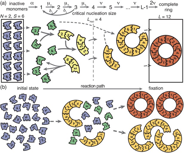
Schematic description of the model.

(a) Rings of size $L$ are assembled from $S$ different particle species. $N$ monomers of each species are initially in an inactive state (blue) and are activated at the same per-capita rate $α$ . Once active (green), species with periodically consecutive index can bind to each other. Structures grow by attachment of single monomers. Below a critical nucleation size ( $L_{nuc}$ ), structures of size $l$ (light yellow) grow and decay into monomers at size-dependent rates $μ_{l}$ and $δ_{l}$ , respectively. Above the critical size, polymers (dark yellow) are stable and grow at size-independent rate $ν$ until the ring is complete (the absorbing state; red). (b) Illustration of depletion traps. If nucleation is slow compared to growth, initiated structures are likely to be completed. Otherwise, many stable nuclei will form that cannot be completed before resources run out.

Figure 2

Download asset Open asset

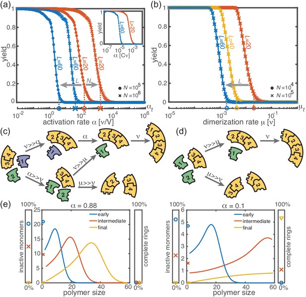
Deterministic behavior in the macroscopic limit $N ≫ 1$ .

(a, b) Yield for different particle numbers $N$ (symbols) and ring sizes $L$ (colors) for $L_{nuc} = 2$ . Decreasing either (a) the activation rate (‘activation scenario’: $μ = ν$ ) or (b) the dimerization rate (‘dimerization scenario’: $α \to \infty$ ) achieves perfect yield. The stochastic simulation results (symbols) average over 16 realizations and agree exactly with the integration of the chemical rate equations (lines). The threshold values (Equation 1) are indicated by the vertical dashed lines. Plotting yield against the dimensionless quantity $α / (ν C)$ causes the curves for different $C$ to collapse into a single master curve (inset in a). For both scenarios there is no dependency on the number of species $S$ in the deterministic limit. (c, d) Illustration showing how depletion traps are avoided by either slow activation (c) or slow dimerization (d). If the activation or the dimerization rate is small (large) compared to the growth rate, assembly paths leading to complete rings are favored (disfavored). The color scheme is the same as in Figure 1. (e) Deterministically, the size distribution of polymers behaves like a wave, and is shown for large and small activation rate for $L = 60$ , $L_{nuc} = 2$ , $N = 10000$ and $μ = ν = 1$ . The distributions are obtained from a numerical integration of the deterministic mean-field dynamics, Equation 6, and are plotted for early, intermediate and final simulation times. The respective percentage of inactive monomers and complete rings is indicated by the symbols in the scale bar on the left or right.

Figure 3

Download asset Open asset

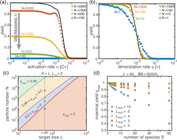
Stochastic effects in the case of reduced resources.

(a, b) Yield of the fully heterogeneous system ( $S = L$ ) for reduced number of particles (symbols) for $L = 60$ and $L_{nuc} = 2$ averaged over 1024 ensembles. In the activation scenario, at low activation rates the yield saturates at an imperfect value $y_{\max}$ , which decreases with the number of particles (a). This finding disagrees with the deterministic prediction (black line) of perfect yield for $α \to 0$ . In contrast, the dimerization scenario robustly exhibits the maximal yield of 1 for small $N$ , in agreement with the deterministic prediction (black line) (b). (c) Diagram showing different regimes of $y_{\max} (N, L)$ in dependence of the particle number $N$ and target size $L$ (for the fully heterogeneous system $S = L$ ) as obtained from stochastic simulations in the limit $α \to 0$ . The minimal number of particles necessary to obtain a fixed yield increases in a strongly nonlinear way with the target size. The symbols along the line $L = 60$ represent the saturation values of the yield curves in (a). (d) Dependence of $y_{\max}$ on the number of species $S$ for fixed $L = 60$ and fixed number of ring structures $N S / L$ . Symbols indicate different values of the critical nucleation size $L_{nuc}$ . The impact of stochastic effects strongly depends on the number of species under the constraint of a fixed total number of particles $N S$ and fixed target size $L$ . The homogeneous system is not subject to stochastic effects at all. Higher reversibility for larger $L_{nuc}$ also mitigates stochastic effects.

Figure 4

Download asset Open asset

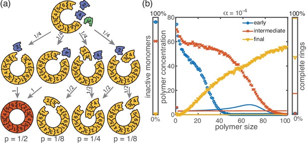
Cause and effect of stochasticity in the activation scenario.

(a) Illustration of the significance of stochastic effects when resources are sparse. Arrows indicate possible transitions and the probabilities in the depicted situation for sufficiently small activation rate $α$ . For small $α$ , the random order of activation alone determines the availability of monomers and therefore the order of binding. In the depicted situation, the complete structure is assembled only with probability 1/2. In all other cases, only fragments of the structure are assembled such that the final yield is decreased. (b) Polymer size distribution for the activation scenario (symbols) as obtained from stochastic simulations, in comparison with its deterministic prediction (lines) for $S = L = 100$ , $N = 1000$ and $L_{nuc} = 2$ . Due to the enhanced number of nucleation events, the stochastic wave encompasses far more structures and moves more slowly. As a result, it does not quite reach the absorbing boundary.

Figure 5

Download asset Open asset

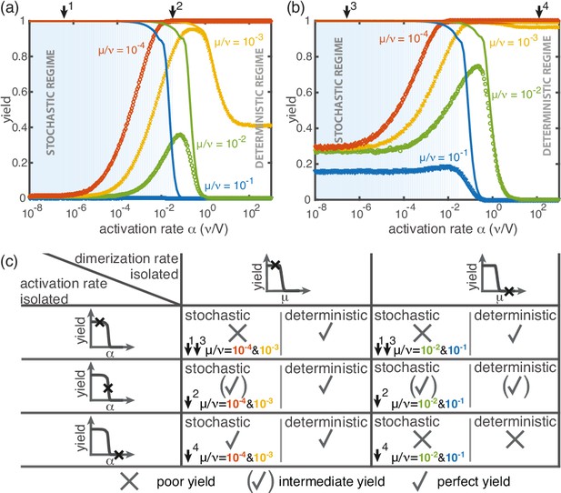
Yield for a combination of slow dimerization and activation.

(a, b) Dependence of the yield of the fully heterogeneous system on the activation rate $α$ for $N = 100$ and different values of the dimerization rate (colors/symbols) for $L = 60$ (a) and $L = 40$ (b) (averaged over 1024 ensembles). For large activation rates the yield behaves deterministically (lines). In contrast, for small activation rates, stochastic effects (blue shading) lead to a decrease in yield. Depending on the parameters, the yield maximum is attained in either the deterministic, stochastic or intermediate regime. (c) Table summarizing the qualitative behavior of the yield (poor/intermediate/perfect) for a combination of dimerization and activation rates for both the deterministic and the stochastic limit. The columns correspond to low and high values of the dimerization rate, as indicated by the marker in the corresponding deterministic yield curve at the top of the column. Similarly, the rows correspond to low, intermediate and high activation rates. Arrows and colors indicate where and for which curve this behavior can be observed in (a) and (b). Deviations between the deterministic and stochastic limits are most prominent for low activation rates.

Figure 6

Download asset Open asset

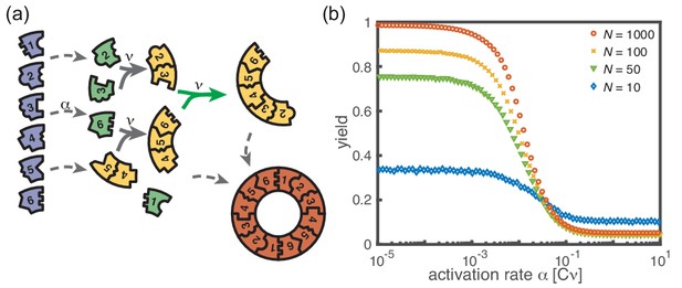
Extended model including polymer-polymer binding.

(a) In the extended model, structures not only grow by monomer attachment but also by binding with another polymer (colored arrow). As before, binding only happens between periodically consecutive species with rate $ν$ per binding site. So, the reaction rate for two polymers is identical to the one for monomer-polymer binding, $ν$ . Furthermore, only polymers with combined length $\leq L$ can bind. All other processes and rules are the same as in the original model described in Figure 1. (b) The yield of the extended model as obtained from stochastic simulations is shown in dependence of the activation rate $α$ for $S = L = 100$ , $μ = ν = 1$ , $L_{nuc} = 2$ and different values of the number of particles per species, $N$ (averaged over 1024 ensembles). The qualitative behavior is the same as for the original model. In particular, yield saturates (in the stochastic limit) at an imperfect value for slow activation rates. Note that for small particle numbers polymer-polymer binding results in an increase of the minimal yield (here for large activation rates). This is due to the fact that even in the case where a priori too many nucleation events happen, polymers can combine into final structures.

Figure 7

Download asset Open asset

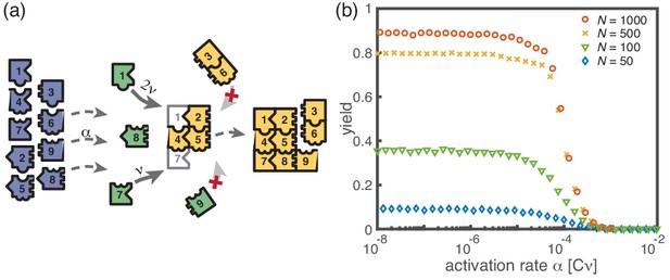
Assembly of squares of size $\sqrt{L} \times \sqrt{L}$ from $L$ different particle species.

(a) As in the ring models, there are $N$ monomers of each species in the system. All particles are initially in an inactive state (blue) and are activated at the same per-capita rate $α$ . Once active (green), species with neighboring position within the square (left/right, up/down) can bind to each other. Structures grow by attachment of single monomers until the square is complete (absorbing state). Depending on the number $b$ of contacts between the monomer and the structure, the corresponding rate is $b ν$ . For simplicity, all polymers (yellow) are stable ( $L_{nuc} = 2$ ) and we do not consider polymer-polymer binding. (b) The yield of the square model as obtained from stochastic simulations is shown in dependence of the activation rate $α$ for $S = L = 100$ , $μ = ν = 1$ and different values of the number of particles per species, $N$ (averaged over 256 ensembles). The qualitative behavior is the same as for the previous models: Whereas the yield is poor for large activation rates, it strongly increases below a threshold value and saturates (in the stochastic limit) at an imperfect value < 1 for small activation rates. The saturation value decreases with decreasing number of particles in the system.

Figure 8

Download asset Open asset

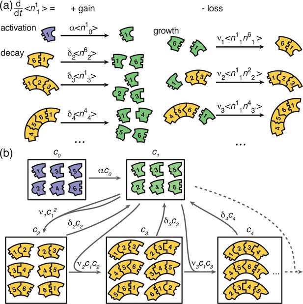
Graphical illustration of Equations 2 and 6.

(a) Visualization of the gain and loss terms in the dynamics of the active monomers in Equation 2b. Gain of active monomers is due to activation of inactive monomers as well as decay of unstable polymers. Loss of active monomers is due to dimerization and attachment of monomers to larger polymers. (b) Visualization of the transitions between clusters of different sizes (without distinction of species). The first and second box represent the inactive and active monomers in the system, the subsequent boxes each represent the ensemble of polymers of a certain size. The arrows between the boxes show possible reactions and transitions with the reaction rates indicated accordingly. Each arrow starting from or leading to a box is associated with a corresponding loss or gain term on the right hand side of Equation 2 and Equation 6.

Appendix 3—figure 1

Download asset Open asset

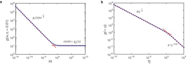
Fit of $g (ω, η)$ on log-log scale.

The function $g (ω, η) = \int_{0}^{\infty} A_{ω, η} (t) 𝑑 t$ describes (half) the travelled distance of the profile of the polymer size distribution in dependence of $ω = \frac{α}{ν C}$ and $η = \frac{μ}{ν}$ . Marker points show solutions for $g (ω, η)$ as obtained numerically from integration of Equation A26. Red lines are linear fits on log-log scale. In (a) we plot $g (ω, η)$ for fixed $η$ (here exemplarily for $η = 0.01$ ) over 25 orders of magnitude in $ω$ and find a markedly bipartite behavior: For small $ω$ the dependence on $ω$ is perfectly matched by a power law with exponent $- \frac{1}{3}$ and $η$ -dependent coefficient $g_{1} (η)$ , whereas for large $ω$ it is a constant $g_{2} (η)$ . (b) Plotting $g_{2} (η) = g (ω = \infty, η)$ in dependence of $η$ reveals again strictly bipartite behavior. Here, however, only the branch for small $η \leq 1$ is relevant. With the coefficient $g_{1} (η)$ that can be determined in a similar way this leads to the final form of $g (ω, η)$ as given by Equation A46.

Appendix 4—figure 1

Download asset Open asset

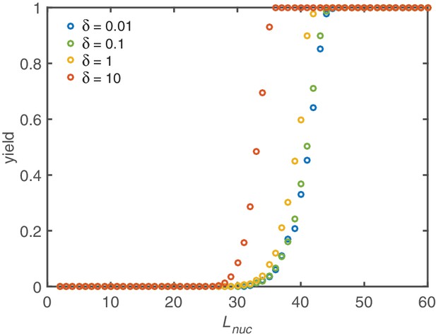
Yield maximization due to increased nucleation size.

Without activation and dimerization mechanism $(α \to \infty, μ = ν)$ the yield can still be optimized by increasing the critical nucleation size $L_{n u c}$ . However, a significant improvement is only achieved for critical sizes larger than half the ring size. Above, a rapid transition to perfect yield takes place. Below no effect is observed at all. Increasing $δ$ shifts the onset of yield to slightly smaller critical nucleation sizes. Other parameters: $L = 60$ , $N = 10000$ .

Appendix 4—figure 2

Download asset Open asset

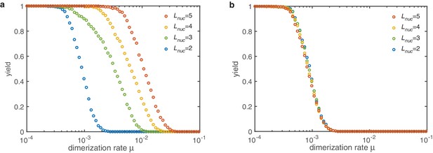
Yield for the dimerization mechanism ( $α \to \infty$ ) with different nucleation sizes (colors).

(a) If all sub-nucleation growth rates are identical $(μ_{i} = μ)$ increasing the nucleation size increases the threshold value $μ_{t h}$ . The slow down of nucleation due to the individual sub-nucleation steps in total determines the yield. (b) If the sub-nucleation growth rates increase linearly $(μ_{i} = μ + (ν - μ) \frac{i - 1}{L_{n u c} - 1})$ no dependence on the nucleation size is observed. The dimerization rate $μ_{1} = μ$ (which is the most limiting step) dominates entirely. Other parameters: $L = 60$ , $N = 10000$ , $δ = 1$ .

Appendix 4—figure 3

Download asset Open asset

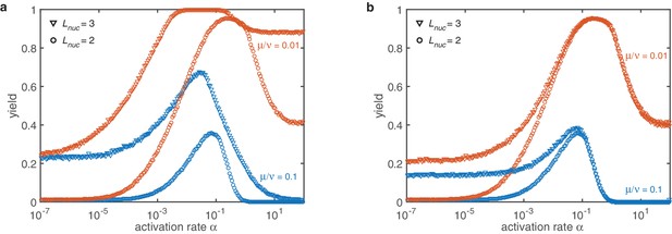
Combined mechanisms for different nucleation sizes (symbols) and dimerization rates (color).

(a) If the sub-nucleation growth rates are identical $(μ_{i} = μ)$ the stochastic yield catastrophe is weakened but still has a drastic impact. The qualitative behavior remains unchanged. (b) For a linearly increasing sub-nucleation growth rate $(μ_{i} = μ + (ν - μ) \frac{i - 1}{L_{n u c} - 1})$ in the deterministic regime no changes are observed at all. The effect of the stochastic yield catastrophe is less pronounced. This improvement is mainly caused by structure decay which mitigates stochastic fluctuations. However, a slight dependency of the saturation value on the rate $μ$ is observed. Other parameters: $L = 60$ , $S = L$ , $N = 100$ , $δ = 0.1$ .

Appendix 5—figure 1

Download asset Open asset

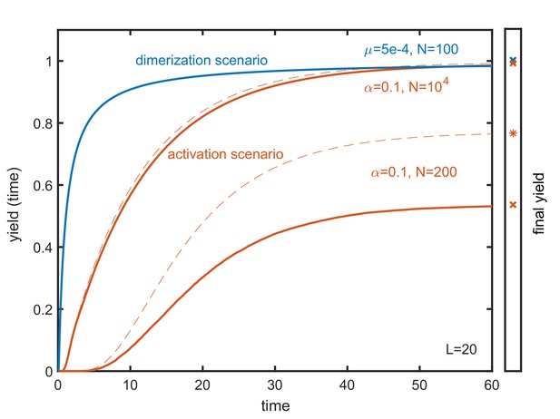
Time evolution of the yield in the activation and dimerization scenario.

The time dependence of the yield is depicted for a dimerization scenario (blue) with $μ = 5 \times 10^{- 4}$ and $N = 100$ and for two activation scenarios (red) with $α = 0.1$ and $N = 2 \times 10^{2}$ and $N = 10^{4}$ , respectively, for target structures of size $L = 20$ . Drawn lines show the time evolution of the stochastic systems while dashed lines describe the time evolution in the corresponding deterministic systems (where the final yield may be higher in the activation scenario). In all cases the yield increases monotonically with time. The final yield, that is indicated in the right bar, represents the upper limit of the yield at any time. Yield production in the activation scenario is generally more gradual than in the dimerization scenario. Therefore, the dimerization scenario is, in general, more time efficient than the activation scenario.

Appendix 6—figure 1

Download asset Open asset

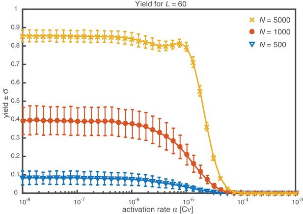
Average yield and its sample standard deviation.

For average yield close to 0 or close to 1, the standard deviation has to be small due to the boundedness of the yield to the interval [0, 1]. For intermediate values, the standard deviation is highest. Its value is, however, still considerably smaller than the average yield. The parameters are $L = 60$ , $S = L$ , $μ = ν = 1$ and different particle numbers $N$ (colors/symbols). To obtain the average yield, the yield has been averaged over 1000 simulations. The standard deviation corresponds to the unbiased sample standard deviation.

Appendix 7—figure 1

Download asset Open asset

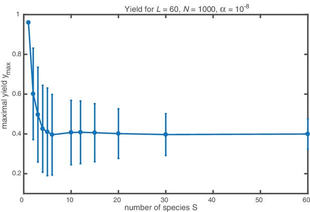
Influence of the heterogeneity of the target structure on the yield for fixed number of particles per species $N$ .

The maximal yield and its standard deviation (obtained as average yield and sample standard deviation for $α = 10^{- 8}$ ) are plotted against the number of species $S$ making up the structure of size $L = 60$ . The number of particles per species $N = 1000$ is fixed. Yield drops from a perfect value of 1 for $S = 1$ to a smaller value and levels off for $S ≫ 1$ . The standard deviation is largest for small $S$ (except for $S = 1$ where the yield is always perfect) and decreases with increasing number of species.

Appendix 8—figure 1

Download asset Open asset

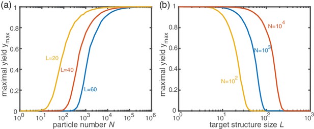
Dependence of the maximal yield $y_{𝐦𝐚𝐱}$ in the activation scenario on $N$ and $L$ .

For each data point, $y_{max}$ was determined as the average yield of 100 independent stochastic simulations of the activation scenario with $α = 10^{- 12}$ . (a) Variation of the particle number $N$ for different target sizes $L$ . The maximal yield increases from 0 to 1 over roughly three order of magnitude in $N$ . The onset of the transition depends on $L$ . (b) Variation of the target size $L$ for different particle numbers $N$ . Increasing the target size $L$ with $N$ being fixed causes the maximal yield to drop to 0. The transition from 1 to 0 spans roughly one order of magnitude in $L$ and its position is determined by $N$ .

Additional files

Source code 1 C++ code for original ring model without polymer-polymer binding.: https://cdn.elifesciences.org/articles/51020/elife-51020-code1-v2.zip
Download elife-51020-code1-v2.zip
Source code 2 C++ code for extended ring model with polymer-polymer binding.: https://cdn.elifesciences.org/articles/51020/elife-51020-code2-v2.zip
Download elife-51020-code2-v2.zip
Source code 3 C++ code for square model.: https://cdn.elifesciences.org/articles/51020/elife-51020-code3-v2.zip
Download elife-51020-code3-v2.zip
Source code 4 MATLAB code for original ring model.: https://cdn.elifesciences.org/articles/51020/elife-51020-code4-v2.zip
Download elife-51020-code4-v2.zip
Transparent reporting form: https://cdn.elifesciences.org/articles/51020/elife-51020-transrepform-v2.pdf
Download elife-51020-transrepform-v2.pdf

Download links

A two-part list of links to download the article, or parts of the article, in various formats.

Downloads (link to download the article as PDF)

Article PDF

Open citations (links to open the citations from this article in various online reference manager services)

Mendeley

Cite this article (links to download the citations from this article in formats compatible with various reference manager tools)

Florian M Gartner
Isabella R Graf
Patrick Wilke
Philipp M Geiger
Erwin Frey

(2020)

Stochastic yield catastrophes and robustness in self-assembly

eLife 9:e51020.

https://doi.org/10.7554/eLife.51020

Sign up for email alerts

Privacy notice