Stable task information from an unstable neural population
- Department of Engineering, University of Cambridge, United Kingdom
- Department of Electrical Engineering, Stanford University, United States
- Department of Neurobiology, Harvard Medical School, United States
Figures
Figure 1
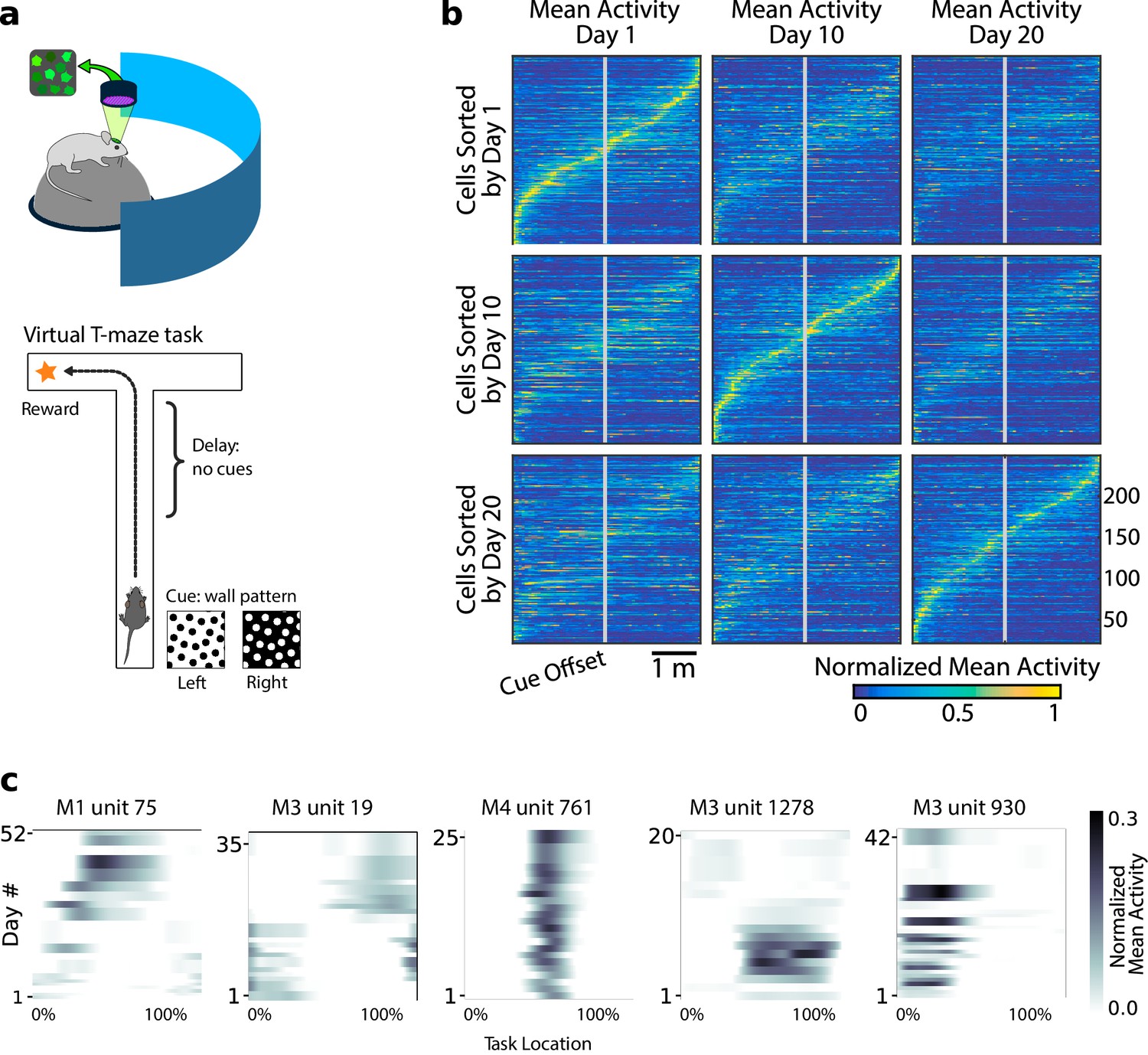
Neural population coding of spatial navigation reconfigures over time in a virtual-reality maze task.
(a) Mice were trained to use visual cues to navigate to a reward in a virtual-reality maze; neural population activity was recorded using Ca2+ imaging Driscoll et al., 2017. (b) (Reprinted from Driscoll et al., 2017) Neurons in PPC (vertical axes) fire at various regions in the maze (horizontal axes). Over days to weeks, individual neurons change their tuning, reconfiguring the population code. This occurs even at steady-state behavioral performance (after learning). (c) Each plot shows how location-averaged normalized activity changes for single cells over weeks. Missing days are interpolated to the nearest available sessions, and both left and right turns are combined. Neurons show diverse changes in tuning over days, including instability, relocation, long-term stability, gain/loss of selectivity, and intermittent responsiveness.
© 2017 Elsevier. Panel B reprinted from Driscoll et al., 2017 with permission from Elsevier. They are not covered by the CC-BY 4.0 licence and further reproduction of this panel would need permission from the copyright holder.
Figure 2 with 1 supplement

A linear decoder can extract kinematic information from PPC population activity on a single day.
(a) Example decoding performance for a single session for mice 4 and 5. Grey denotes held-out test data; colors denote the prediction for the corresponding kinematic variable. (b) Summary of the decoding performance on single days; each point denotes one mouse. Error bars denote one standard deviation over all sessions that had at least high-confidence PPC neurons for each mouse. (Mouse two is excluded due to an insufficient number of isolated neurons). Chance level is ∼1.5 m for forward position, and varies across subjects for forward velocity (∼0.2–0.25 m/s) and head direction (∼20-30 ). (c) Extrapolation of the performance of the static linear decoder for decoding position as a function of the number of PPC neurons, done via Gaussian process regression (Materials and methods). Red '×' marks denote data; solid black line denotes the inferred mean of the GP. Shaded regions reflect ±1.96σ Gaussian estimates of the 95th and 5th percentiles. (d) Same as panel (c), but where the neurons have been ranked such that the ‘best’ subset of size 1≤K≤N is chosen, selected by greedy search based on explained variance (Materials and methods: Best K-Subset Ranking).
Figure 2—figure supplement 1
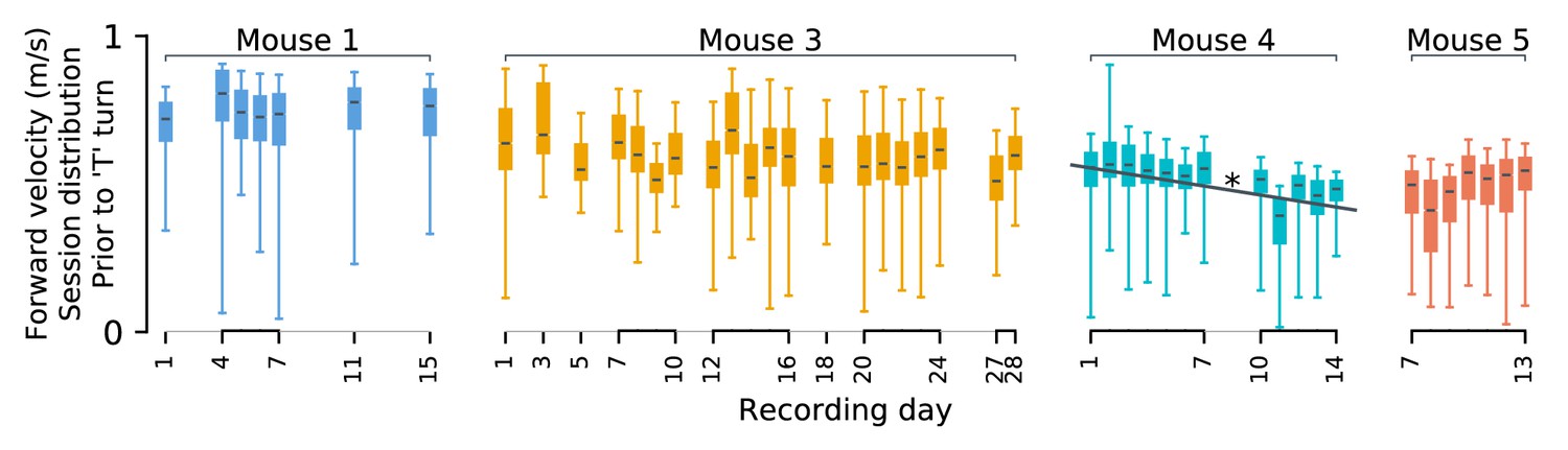
Behavioral stability.
Statistics of forward motion show small daily variations. It is possible that changes in population codes relate to systematic changes in behavior over time. As described in Driscoll et al., 2017, these experiments were performed only after mice achieved asymptotic performance in speed and accuracy. Nevertheless, there is some behavioral variability. Each mouse’s velocity in the initial (forward) segment of the ‘T’ maze varies slightly between days. Differences in means (black lines) are often statistically significant (p<0.05 in 91% pairs of sessions; Bonferroni multiple-comparison correction for a 0.05 false discovery rate), but are small ( i.e. Cohen’s d ranges between 10–16% per animal). Systematic drift-like trends appear absent from mice 1 and 3. A statistically significant trend is present for mouse 4 (Pearson’s ρ = − 0.9, p<0.05). We show only forward velocity here, as other kinematics variables exhibited less variability. Daily fluctuations in behavior could be used to weakly predict the recording session. Under cross-validation, linear discriminant analysis based on ten-second windows of kinematics predicted the recording session 9–17% above chance. This suggests that each mouse exhibited small but detectable daily variability in their behavior. Most variability was unsystematic, and therefore unrelated to the slow changes in neural codes studied here. We expect changes in forward speed in mouse four to contribute to apparent drift in some cells. However, the results presented here generalize across mice 1, 3, and 5, which exhibited stable behavior.
Figure 3
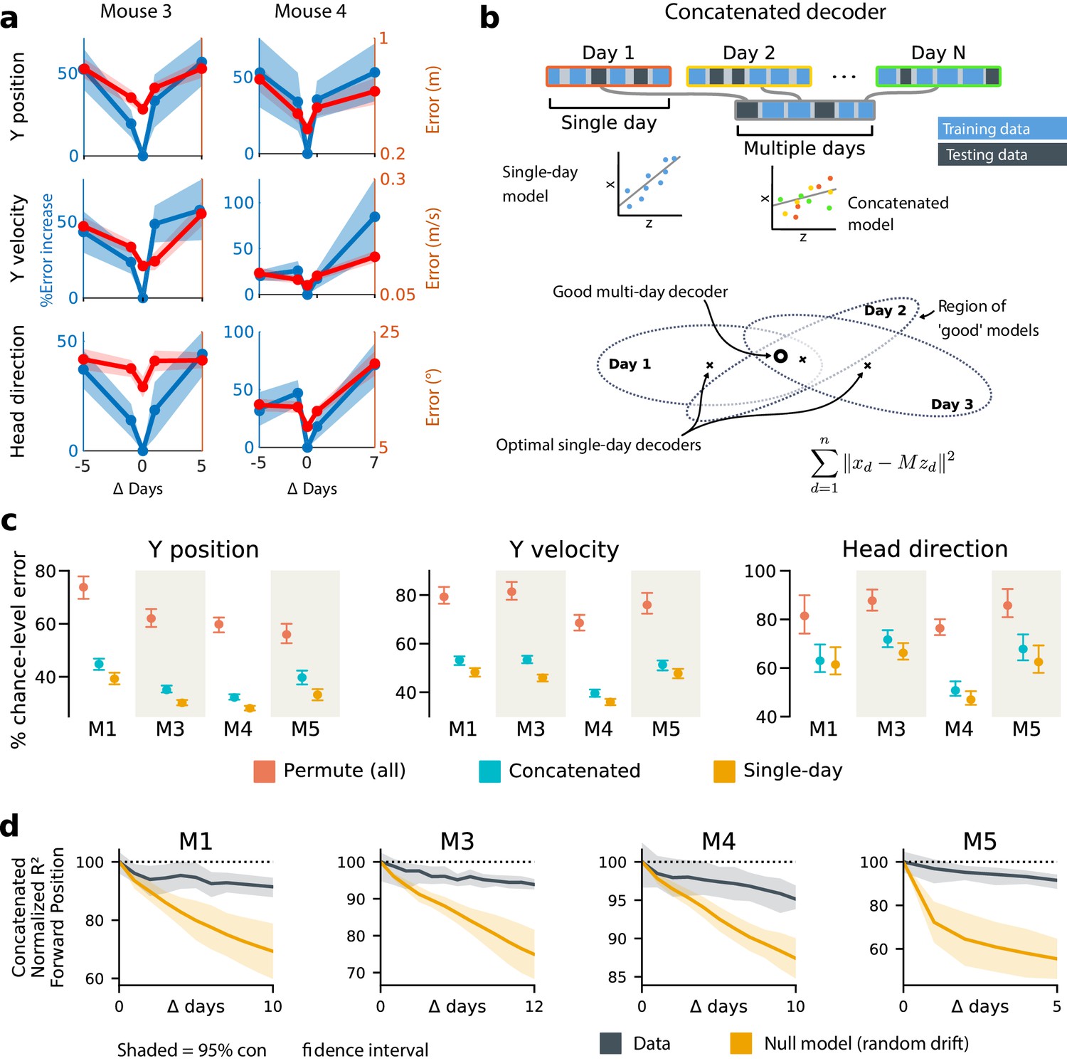
Single-day decoders generalize poorly to previous and subsequent days, but multi-day decoders exist with good performance.
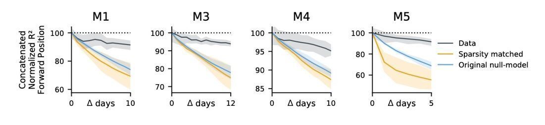
(a) Blue: % increase in error over the optimal decoder for the testing day (mouse 3, 136 neurons; mouse 4, 166 neurons). Red: Mean absolute error for decoders trained on a single day (‘0’) and tested on past/future days. (b) Fixed decoders for multiple days (‘concatenated decoders’) are fit to concatenated excerpts from several sessions. The inset equation reflects the objective function to be minimized (Methods). Due to redundancy in the neural code, many decoders can perform well on a single day. Although the single-day optimal decoders vary, a stable subspace with good performance can exist. (c) Concatenated decoders (cyan) perform slightly but significantly worse than single-day decoders (ochre; Mann-Whitney U test, p<0.01). They also perform better than expected if neural codes were unrelated across days (permutation tests; red). Plots show the mean absolute decoding error as a percent of the chance-level error (points: median, whiskers: 5th–95th%). Chance-level error was estimated by shuffling kinematics traces relative to neural time-series (mean of 100 samples). For the permutation tests, 100 random samples were drawn with the neuronal identities randomly permuted. (d) Plots show the rate at which concatenated-decoder accuracy (normalized ) degrades as the number of days increase. Concatenated decoders (black) degrade more slowly than expected for random drift (ochre). Shaded regions reflect the inner 95% of the data (generated by resampling for the null model). The null model statistics are matched to the within- and between-day variance and sparsity of the experimental data for each animal (Materials and methods).
Figure 4 with 1 supplement
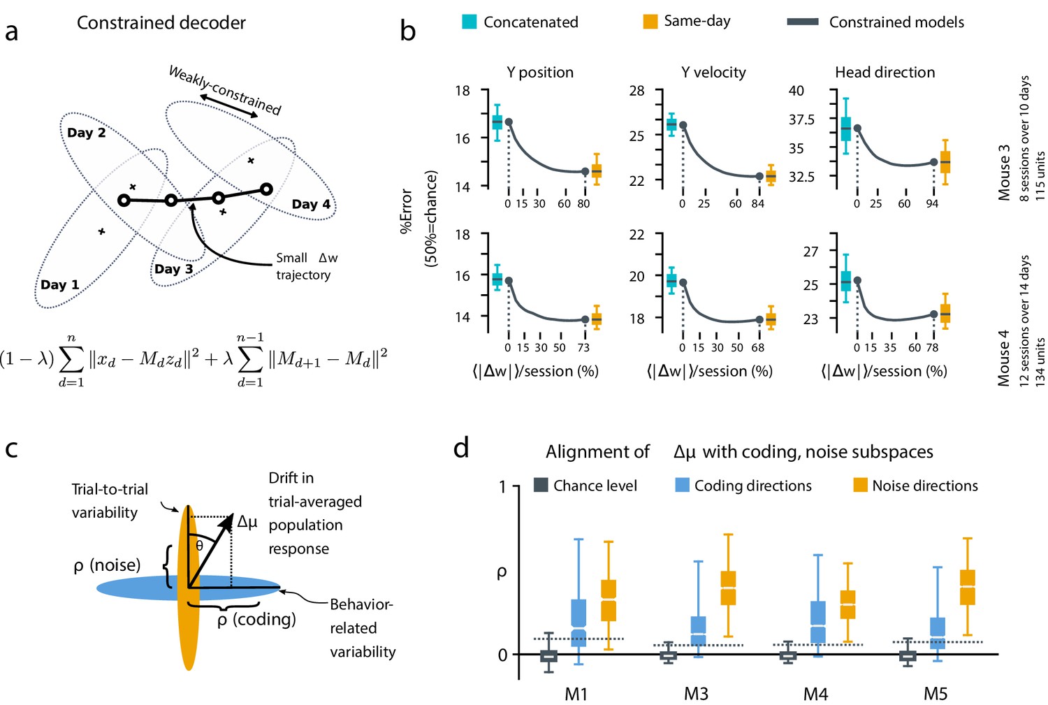
A slowly-varying component of drift disrupts the behavior-coding subspace.
(a) The small error increase when training concatenated decoders (Figure 3) suggests that plasticity is needed to maintain good decoding in the long term. We assess the minimum rate for this plasticity by training a separate decoder for each day, while minimizing the change in weights across days. The parameter λ controls how strongly we constrain weight changes across days (the inset equation reflects the objective function to be minimized; Methods). (b) Decoders trained on all days (cyan) perform better than chance (red), but worse than single-day decoders (ochre). Black traces illustrate the plasticity-accuracy trade-off for adaptive decoding. Modest weight changes per day are sufficient to match the performance of single-day decoders (Boxes: inner 50% of data, horizontal lines: median, whiskers: 5–95th%). (c) Across days, the mean neural activity associated with a particular phase of the task changes (). We define an alignment measure (Materials and methods) to assess the extent to which these changes align with behavior-coding directions in the population code (blue) verses directions of noise correlations (ochre). (d) Drift is more aligned with noise (ochre) than it is with behavior-coding directions (blue). Nevertheless, drift overlaps this behavior-coding subspace much more than chance (grey; dashed line: 95% Monte-Carlo sample). Each box reflects the distribution over all maze locations, with all consecutive pairs of sessions combined.
Figure 4—figure supplement 1
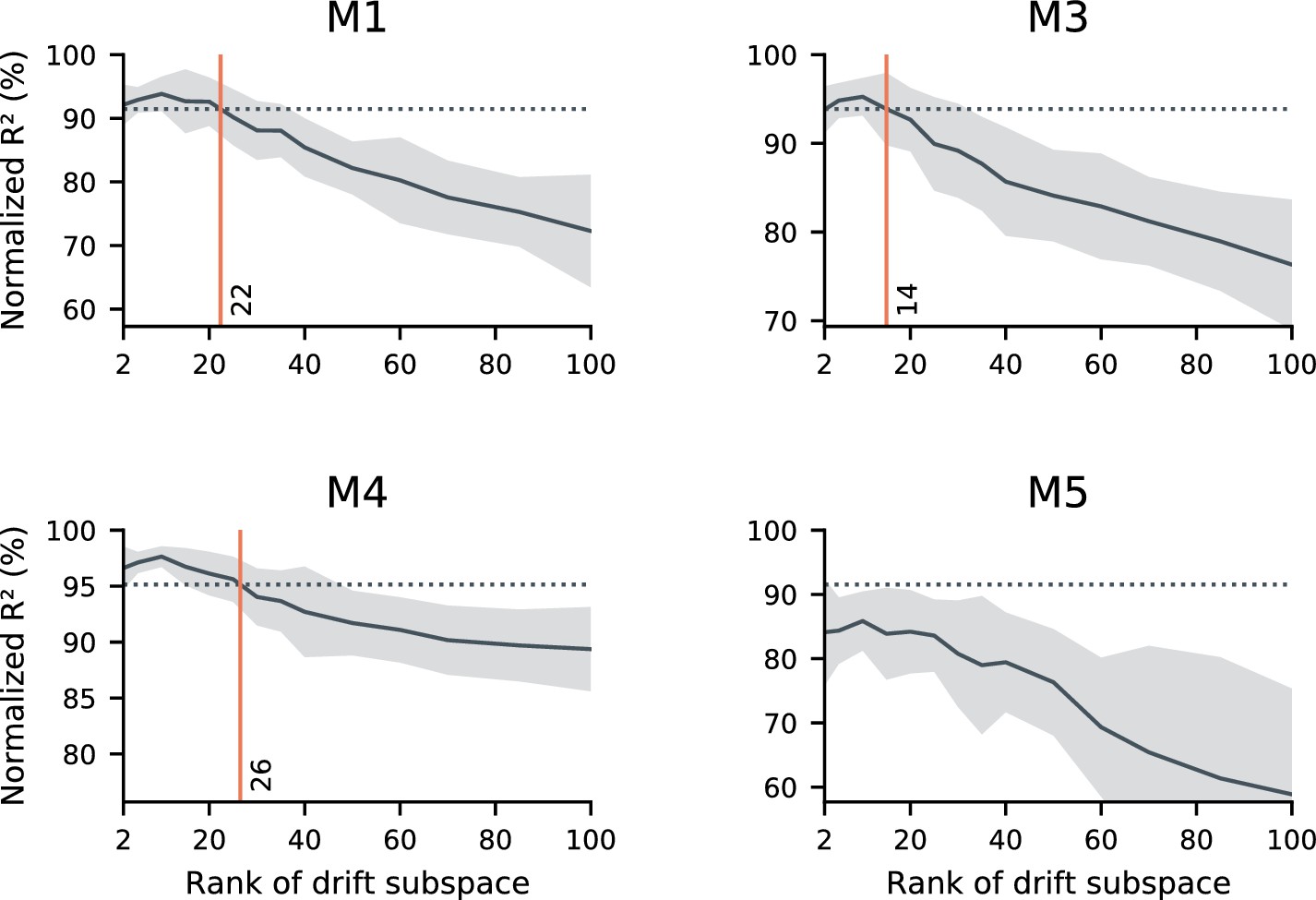
Concatenated decoder performance depends on the rank of the drift.
sufficiently low-rank drift resembles the data in terms of the performance of a concatenated decoder. Here, we further explore the null model introduced in Figure 3d. As in Figure 3d, we simulated random drift in the neural readout. We matched the null model to the statistics of neural activity, the within-day decoding accuracy, and the performance degradation when generalizing between days. In these simulations, we explore the scenario that the drift may be confined to a (randomly-selected) low-dimensional subspace. We evaluated a range of dimensionalities for the drift subspace (horizontal axes), and evaluated the performance of a concatenated decoder on simulated data. While unconstrained drift prevents the identification of a concatenated decoder with good performance (Figure 3d), sufficiently constrained drift does not. In these simulations, we found that constraining drift to a subspace of rank 14–26 (red vertical lines) led to similar performance as the data (dashed horizontal lines) in all subjects except for mouse 5. We speculate that this is because Mouse five had limited data and poor generalization of single-day decoders over time, but other scenarios are possible. Black traces reflect the mean over 20 random simulations, and shaded regions reflect one standard deviation.
Figure 5 with 3 supplements
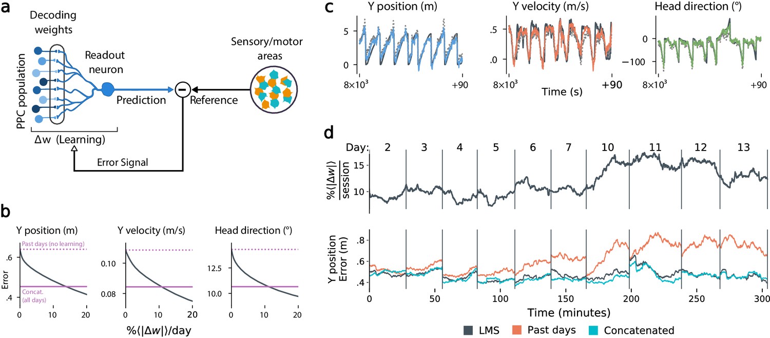
Local, adaptive decoders can track representational drift over multiple days.
(a) The Least Mean-Squares (LMS) algorithm learns to linearly decode a target kinematic variable based on error feedback. Continued online learning can track gradual reconfiguration in population representations. (b) As the average weight change per day (horizontal axis) increases, the average decoding error (vertical axis) of the LMS algorithm improves, shown here for three kinematic variables (Mouse 4, 144 units, 10 sessions over 12 days; Methods: methods:lms). (Dashed line: error for a decoder trained on only the previous session without online learning; Solid line: performance of a decoder trained over all testing days). As the rate of synaptic plasticity is increased, LMS achieves error rates comparable to the concatenated decoder. (c) Example LMS decoding results for three kinematic variables. Ground truth is plotted in black, and LMS estimate in color. Sample traces are taken from day six. Dashed traces indicate the performance of the decoder without ongoing re-training. (d) (top) Average percent weight-change per session for online decoding of forward position (learning rate: 4 × 10⁻⁴/sample). The horizontal axis reflects time, with vertical bars separating days. The average weight change is 10.2% per session. To visualize % continuously in this plot, we use a sliding difference with a window reflecting the average number of samples per session. (bottom) LMS (black) performs comparably to the concatenated decoder (cyan) (LMS mean absolute error of 0.47 m is within ≤ 3% of concatenated decoder error). Without ongoing learning, the performance of the initial decoder degrades (orange). Error traces have been averaged over ten minute intervals within each session. Discontinuities between days reflect day-to-day variability and suggest a small transient increase in error for LMS decoding at the start of each day.
Figure 5—figure supplement 1

Online learning with LMS: additional subjects.
LMS results for mice 1, 3, 4, and 5. Results of applying the online LMS algorithm with a learning rate of 4 × 10⁻⁴/sample. Errors reflect the mean absolute error over ten minute intervals. LMS (black) achieves errors comparable to an offline decoder trained on all sessions ('concatenated’, blue), and outperforms a fixed decoder trained on the initial day (red). Only times within a trial were used for training. For the LMS algorithm, we observed inter-day weight changes of 7.6-10.4%, consistent with observed rates of change in the volume of dendritic spines in other studies. We present two spans of time from Mouse 3, reflecting two largely non-overlapping populations of tracked neurons on non-overlapping spans of days.
Figure 5—figure supplement 2
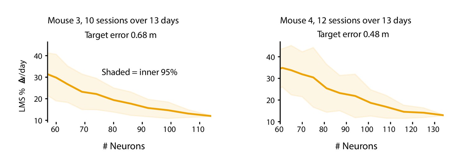
The plasticity level required to track drift varies with population size.
Smaller populations require more plasticity to achieve target error levels. These plots show the daily weight changes required to track drift when decoding forward positions as a function of population size for mice 3 and 4. Smaller populations require more plasticity. The target error (M3: 0.68 m, M4: 0.48 m) was set based on the performance of LMS on the full population (M3: 114 neurons, M4: 134 neurons). For each sub-population size, 50 random sub-populations were drawn, and the learning rate was optimized to achieve the target error level. Shaded regions reflect the inner 95th percentile over all sampled sub-populations. Weight change was assessed as the weight change between the end of consecutive sessions and normalized by the overall average weight magnitude.
Figure 5—figure supplement 3

Extrapolation to larger populations.
The plasticity required to achieve a fixed error level decreases for larger populations. Typically, the number of inputs to a neuron is much larger than the ∼100 neurons observed here. The ∼10% weight change per day reported by LMS could therefore over-estimate of plasticity needed to track drift. To address this, we combined data from multiple mice to extend the LMS analysis to a synthetic population of 1238 cells over six sessions. Trials were matched based on the current and previous cue, and converted to pseudotime based on the fraction of the maze completed between 0 and 100%. We allowed up to two-day recording gaps between consecutive sessions from the same mouse. These synthetic populations are not equivalent to large recordings from a single mouse, but nevertheless reveal how plasticity scales with population size. We found that larger populations could achieve the same performance as ∼100 cells with a ∼4% weight change per day. (a) Trial pseudotime (% of trial complete; black) can be decoded from a synthetic pooled population (1238 cells) using the LMS algorithm (violet: prediction). (b) Similarly to the single-subject results, LMS tracks changes in the population code over time. In this case, a learning rate of 8 × 10⁻⁴/sample achieved comparable error to a concatenated decoder. The larger population permits better decoding error of ∼5%, compared to the ∼15 - 20% error in forward position decoded from ∼100 neurons. (c) As population size increases, both the weight magnitudes (left) and the rates of weight change (middle) decrease. Small populations could not achieve the error rates possible using the full population, even with very large learning rates. We therefore set the target error a bit higher, at 13% chance level. This is comparable to the error rates seen in individual mice using ∼100 cells. Overall, the required percentage weight change decreased for larger populations (right).
Author response image 1
Additional files
Download links
A two-part list of links to download the article, or parts of the article, in various formats.
Downloads (link to download the article as PDF)
Open citations (links to open the citations from this article in various online reference manager services)
Cite this article (links to download the citations from this article in formats compatible with various reference manager tools)
Stable task information from an unstable neural population
eLife 9:e51121.
https://doi.org/10.7554/eLife.51121


