Myosin V executes steps of variable length via structurally constrained diffusion
- Department of Physics, Cornell University, United States
- Department of Physics and Astronomy, Denison University, United States
- Department of Physics, Case Western Reserve University, United States
- Department of Chemistry, University of Texas, United States
Figures
Figure 1

Myosin V geometry.
(A) Side view, with the actin filament plus end oriented toward the direction. Small circles on the actin monomers denote the binding sites , described by Equation 1. The site corresponds to the position of the bound head. The bound polymer leg has a preferred post-power stroke direction in the plane defined by a constraint angle relative to the axis. Due to the hypothesized structural constraint at the joint, the preferred angle between the lever arms is . The force transmitted through the tail domain has a polar angle relative to the direction. (B) Front view, with the actin plus end pointing out of the page. Each binding site has an associated outward pointing normal direction with azimuthal angle . As an example, one such angle is shown for the red-colored site. All azimuthal angles are measured counter-clockwise with respect to the direction. For binding to occur, the head has to be in the vicinity of the site, and oriented approximately along the normal. We approximately capture this condition by a binding criterion that requires the azimuthal angle of the free leg, , to be anti-parallel to within a cutoff range , highlighted in light red. The load force may have an off-axis component with azimuthal angle .
Figure 2
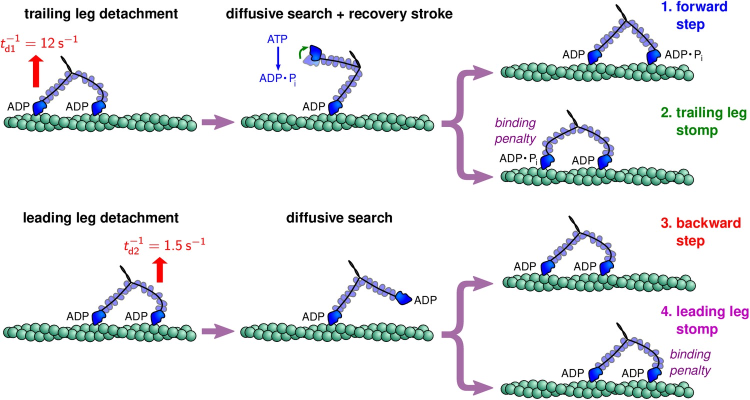
Myosin V kinetic pathways.
Figure 3 with 7 supplements

Contours of the myosin V free head position distribution projected onto the plane.
Top row: theoretical predictions for (A) free diffusion () and (B–D) constrained diffusion with inter-leg constraint strength (B) , (C) , and (D) . Bottom row: the corresponding contours measured from Brownian dynamics simulations, with inter-leg constraint strength (E) , (F) , (G) , and (H) . (I) Experimental measurements of the diffusion by Andrecka et al. (2015). Adding an inter-leg constraint potential produces a multi-peaked diffusion pattern. The heights of the peaks are similar to the experimental measurements for . Note that the axis in the experimental data corresponds to the position of the gold bead attached to the myosin head when the head is bound to actin. Given the ∼5 nm size of the head and ∼10 nm radius of the bead, this accounts for the approximately 15 nm vertical shift between the theoretical/simulation distributions and experiment. In the former the axis corresponds to the top of the actin filament (where the bound head is attached).
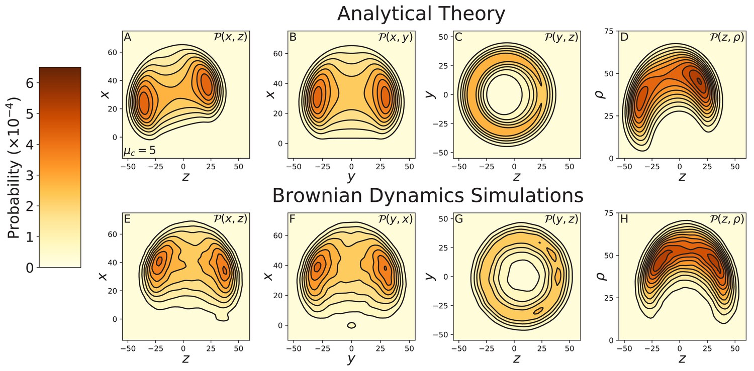
Figure 3—figure supplement 1

Alternative projections of the constrained diffusion ().
Top row: theoretical calculations of the diffusion projected onto the (A) , (B) , and (C) planes, and (D) the cylindrical plane . Bottom row: diffusion contours measured from Brownian dynamics simulations, again projected onto the (E) , (F) , and (G) planes, and (H) the cylindrical plane . Agreement between theory and simulations is excellent.
Figure 3—figure supplement 2

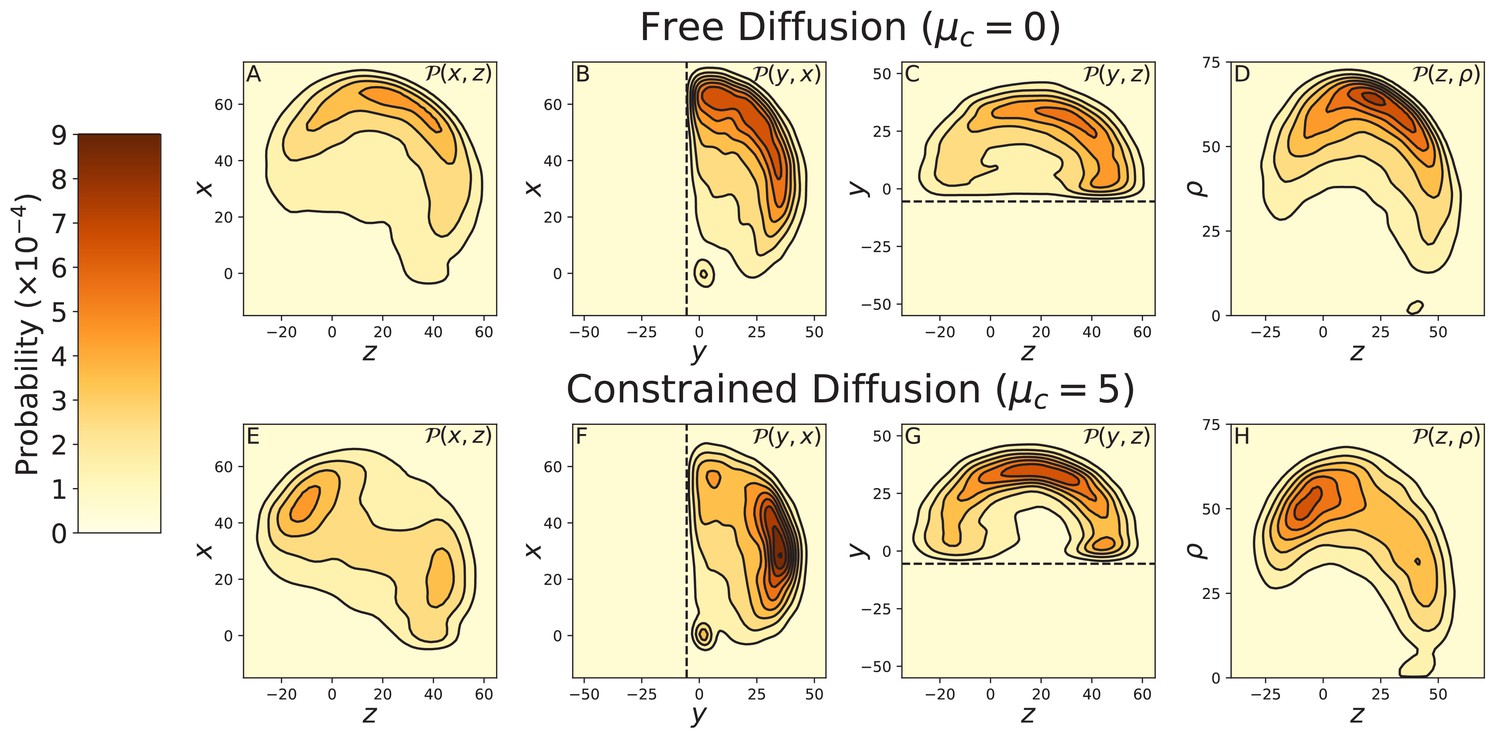
Alternative projections of the free diffusion ().
Top row: theoretical calculations of the diffusion projected onto the (A) , (B) , and (C) planes, and (D) the cylindrical plane . Bottom row: diffusion contours measured from Brownian dynamics simulations, again projected onto the (E) , (F) , and (G) planes, and (H) the cylindrical plane . In the analytical theory we include a joint Hamiltonian that penalizes small inter-leg angles. This mimics the effects of steric repulsion between the legs, which are explicitly included in the BD simulations. With this adjustment to the theory, agreement between the theory and simulations is excellent.
Figure 3—figure supplement 3
Constrained diffusion of myosin V under 2 pN backward force.
The constraint strength was set to . The force = 2 pN is in the stall regime, just above the stall force. Top row: theoretical calculations of the diffusion projected onto the (A) , (B) , and (C) planes, and (D) the cylindrical plane . Bottom row: diffusion contours measured from Brownian dynamics simulations, again projected onto the (E) , (F) , and (G) planes, and (H) the cylindrical plane . The theory and simulations agree qualitatively, showing the diffusion is rotated toward the minus end of the actin compared to that at zero load (Figure 3—figure supplement 1). Quantitative discrepancies are primarily due to a small difference in the stall force between the theoretical and numerical models.
Figure 3—figure supplement 4
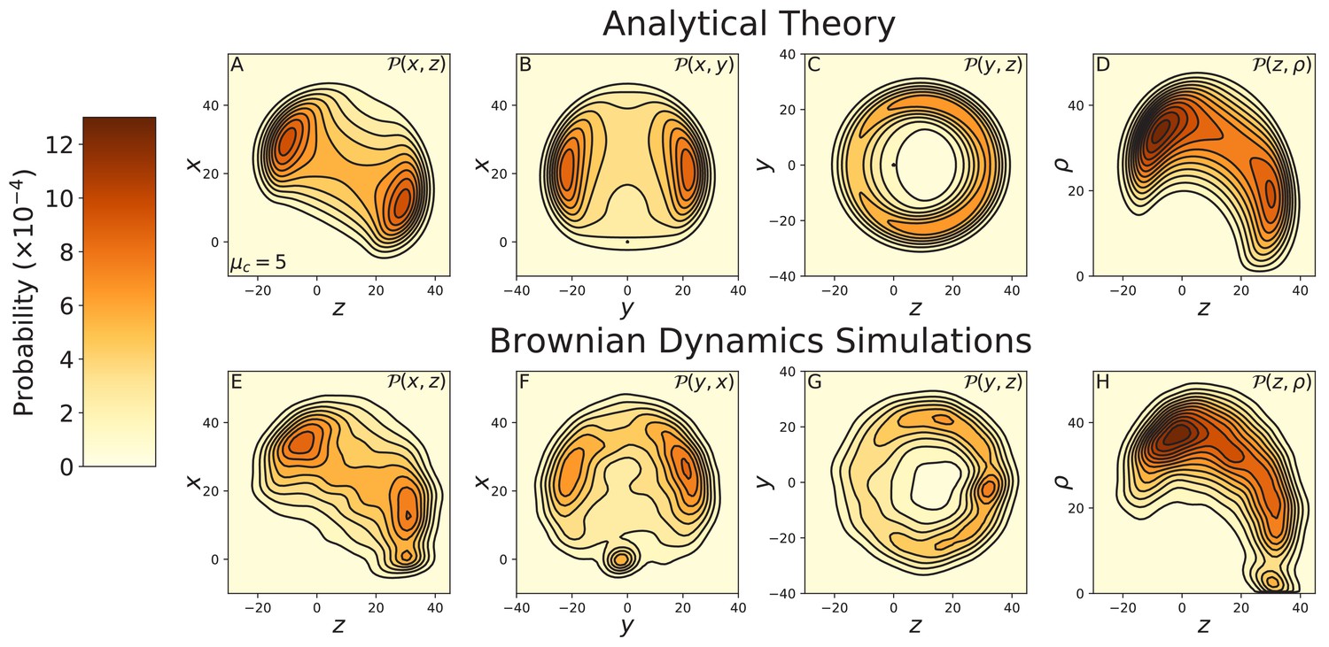
Constrained diffusion of the 4IQ myosin mutant.
The constraint strength was set to . Top row: theoretical calculations of the diffusion projected onto the (A) , (B) , and (C) planes, and (D) the cylindrical plane . Bottom row: diffusion contours measured from Brownian dynamics simulations, again projected onto the (E) , (F) , and (G) planes, and (H) the cylindrical plane . Notice the difference in probability and length scales in this figure versus those preceding. The 4IQ mutant has a nearly identical diffusion pattern to the wild-type myosin, scaled down due to the decreased lever arm length.
Figure 3—figure supplement 5
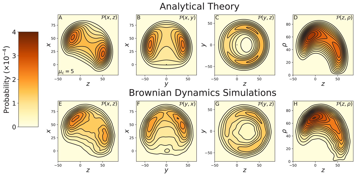
Constrained diffusion of the 8IQ myosin mutant.
The constraint strength was set to . Top row: theoretical calculations of the diffusion projected onto the (A) , (B) , and (C) planes, and (D) the cylindrical plane . Bottom row: diffusion contours measured from Brownian dynamics simulations, again projected onto the (E) , (F) , and (G) planes, and (H) the cylindrical plane . Notice the difference in probability and length scales in this figure versus those preceding. The 8IQ mutant has a nearly identical diffusion pattern to the wild-type myosin, scaled up due to the increased lever arm length.
Figure 3—figure supplement 6
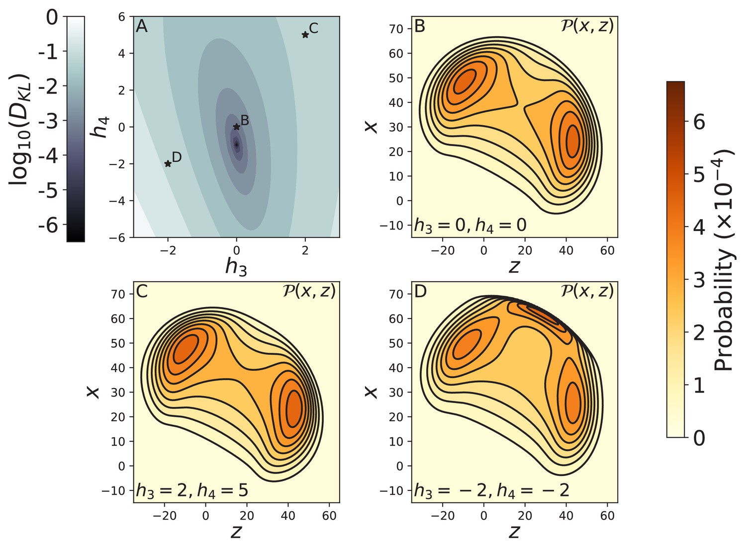
Effect of the form of the joint potential on free head diffusion.
(A) The log of the KL divergence between the free head spatial probability densities and corresponding to the cosine potential used in the main text and respectively. The minimum KL divergence occurs at , which is the quartic expansion of the cosine potential. The stars indicate the potentials used to compute diffusion contours in panels B–D. The diffusion contours are shown for (B) the harmonic potential , as well as potentials with (C) , and (D) . The harmonic potential produces diffusion that is nearly identical to the cosine potential (Figure 3C), while the contour shown in C has only subtle differences. The diffusion shown in D is qualitatively different because the potential has an additional energy minimum giving rise to a new peak in the distribution. In all cases we set , as in the main text.
Figure 3—figure supplement 7
Effects of cover-slip volume exclusion on diffusion.
Data was taken using Brownian Dynamics simulations with a glass cover-slip cutting off half the 3-dimensional space, modeled with a soft-core repulsive potential as described in Appendix 2. The cover-slip is at = —5.5 nm, parallel to the plane and is indicated by the dashed line in the relevant diffusion projections. Top row: BD simulations of free diffusion (), projected onto the (A) , (B) , and (C) planes, and (D) the cylindrical plane . Bottom row: BD simulations of free diffusion (), again projected onto the (E) , (F) , and (G) planes, and (H) the cylindrical plane . The diffusion contour is not considerably altered by the cover-slip in both the free and constrained diffusion models. Therefore, the multi-peaked contour measured by Andrecka et al. (2015) is not an artifact of entropic forces due to volume exclusion.
Figure 4 with 7 supplements
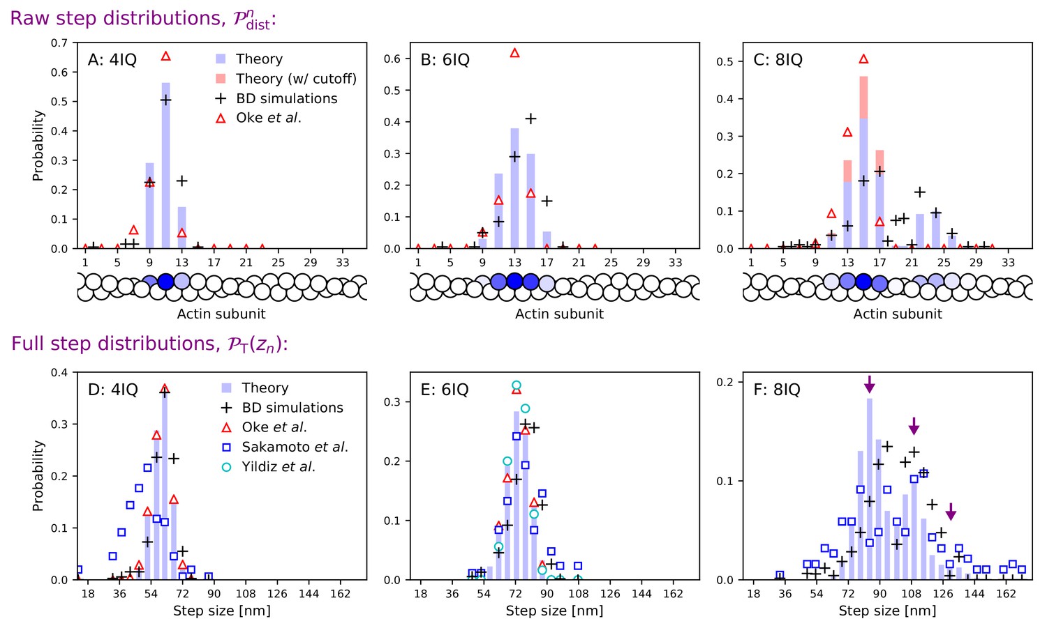
Step size distributions for myosin V and mutants with altered leg length.
Top row: raw step distributions for (A) the 4IQ mutant, (B) the 6IQ wild-type, and (C) the 8IQ mutant. Bottom row: full (convolved) step distributions for (D) the 4IQ mutant, (E) the 6IQ wild-type, and (F) the 8IQ mutant, with three theoretical peak locations indicated by arrows. Theoretical distributions are shown as histograms with Brownian dynamics simulations and experimental data from Oke et al. (2010), Sakamoto et al. (2005), and Yildiz et al. (2003) indicated by symbols. The raw data from Oke et al. (2010) is convolved and binned in the bottom row. Since the imaging methods used in this experiment did not resolve large steps taken by the 8IQ mutant, in panel C we show an alternative theory (in red) with a cutoff where only small steps are allowed. The actin monomers drawn below the top row are shaded according to the analytical theory results, with the darkest color normalized to the peak of the distribution.
Figure 4—figure supplement 1

Step distributions for myosin V and mutants with a freely rotating inter-leg joint.
Same as Figure 4, but analytical theory and Brownian dynamics simulations used the free diffusion model. The analytical model was fit to data using the procedure described in the main text. We used parameters: , , , , , , and , with all other parameters identical to Table 2. Agreement with experimental measurements is comparable to that for the constrained diffusion model.
Figure 4—video 1
BD simulation trajectory illustrating stepping for the 6IQ wild-type.
The myosin dimer is depicted in blue, and the locations of potential myosin binding sites on the two actin filaments are shown in light grey and red. The BD parameters are listed in Appendix 2. This video shows the case for a motor with a freely rotating inter-leg joint making a step where the final head separation is is 36 nm (13 actin subunits).
Figure 4—video 2
BD simulation of stepping for the 6IQ wild-type with a freely rotating joint, but with a longer step (final head separation > 36 nm).
Figure 4—video 3
BD simulation of stepping for the 6IQ wild-type with a freely rotating joint, but with a shorter step (final head separation < 36 nm).
Figure 4—video 4
Similar to Figure 4—video 1, but with an inter-leg joint constraint ().
Figure 4—video 5
Similar to Figure 4—video 2, but with an inter-leg joint constraint ().
Figure 4—video 6
Similar to Figure 4—video 3, but with an inter-leg joint constraint ().
Figure 5 with 1 supplement
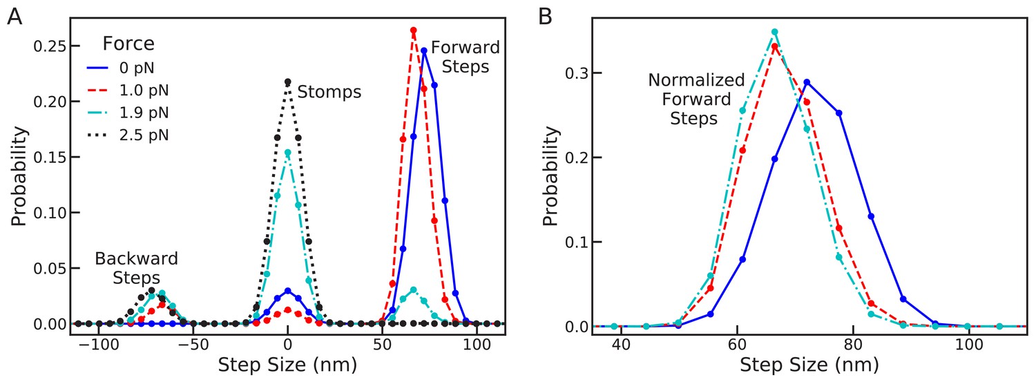
Changes in the full step distribution, including leading and trailing leg contributions, under backward load.
(A) Distributions for zero force = 0 pN (solid line), sub-stall force = 1 pN (dashed line), stall force = 1.9 pN (dot-dashed line), and super-stall force = 2.5 pN (dotted line). The peaks near 72 nm, 0 nm and –72 nm correspond to forward steps, stomps, and backward steps respectively. Applying force shifts the forward step distribution backward slightly (by about 1 actin subunit) and increases the probability of stomps and backward steps. (B) Normalized forward step distributions for = 0 pN, = 1 pN, and = 1.9 pN. Even when other kinetic pathways are dominant the shape of the forward step distribution remains robust to load force.
Figure 5—figure supplement 1

Robust forward step distributions from Brownian dynamics simulations.
Shown are the normalized forward step distribution measured from BD trajectories with zero force and under backward load of 1 pN and 2 pN. The distribution is fairly robust, shifting back about one actin subunit per piconewton of applied force, in qualitative agreement with the analytical model (Figure 5B).
Figure 6
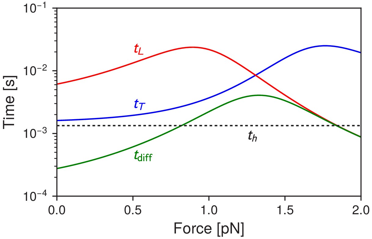
Myosin V timescales as a function of , the backward load force.
is the mean timescale for the detached head to diffuse within radius of any of the actin binding sites. and are the mean times for the trailing and leading heads to bind after detachment. For comparison, is the mean timescale of ATP hydrolysis.
Figure 7
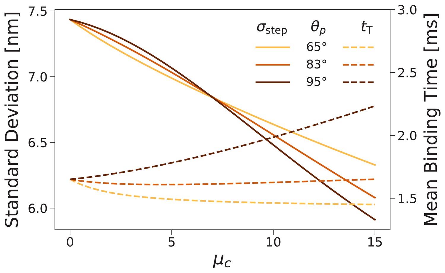
Forward step distribution width (solid lines) and mean binding time after trailing leg detachment (dashed lines) for as a function of the inter-leg constraint strength .
We carried out this calculation for (the value used throughout this paper) as well as and . As the constraint is increased the step distribution narrows, while changes in the binding time are relatively small.
Figure 8 with 1 supplement
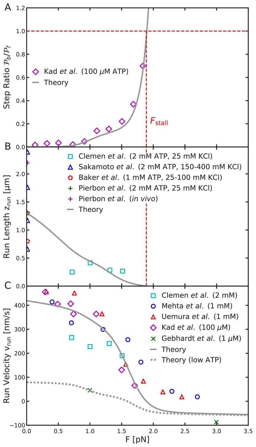
Load-dependent aspects of myosin V dynamics.
(A) Backward-to-forward step ratio ; (B) mean run length ; (C) mean run velocity . Analytical theory results are drawn as curves, experimental results as symbols. The legend symbols are the same as those in Hinczewski et al. (2013), for ease of comparison, but the theory curves have been updated.
Figure 8—figure supplement 1
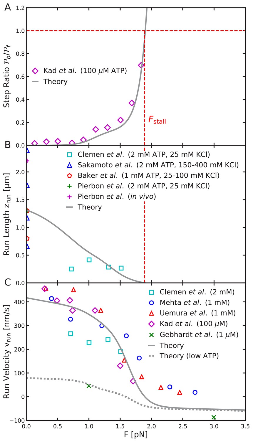
Load-dependence of step ratio, run length, and run velocity is captured by the free diffusion model.
Same as Figure 8, but using the analytical free diffusion model, fit to experiments as described in the main text. We used parameters: , , , , , , and , with all other parameters identical to Table 2. Agreement with experimental measurements is comparable to that for the constrained diffusion model.
Figure 9
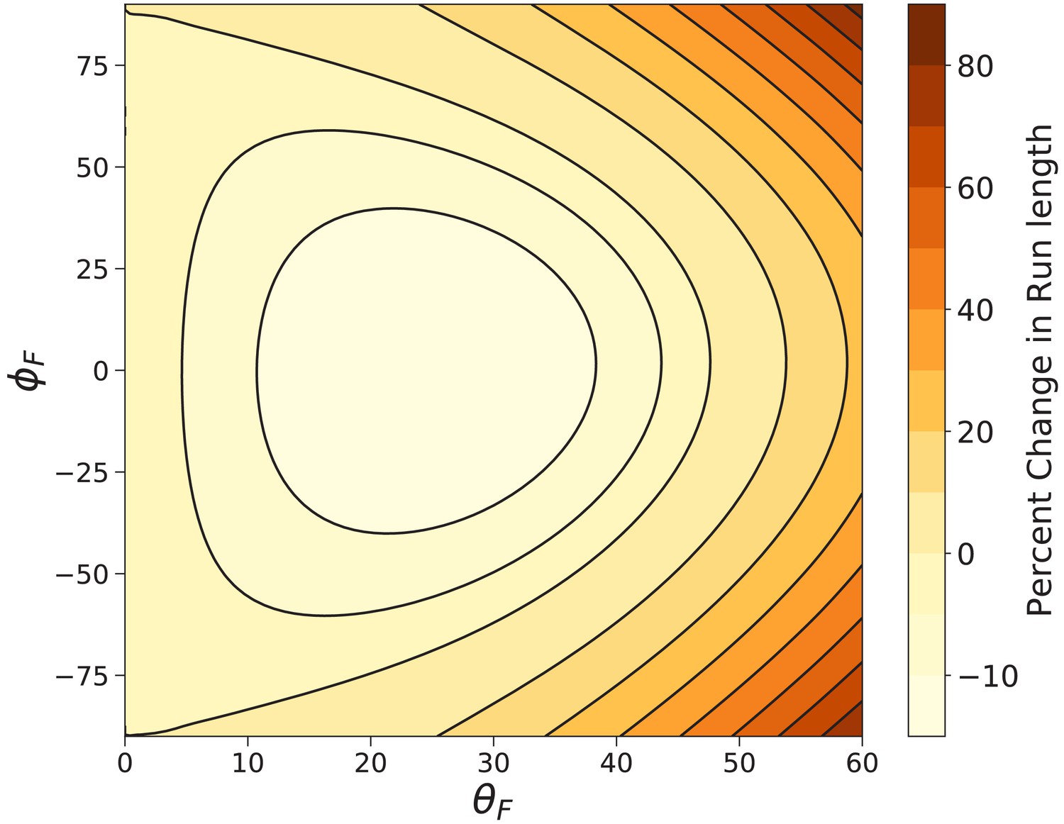
Myosin V run length under off-axis forces.
Shown is the percent change in run length from that under backward force computed using Equation 9. In the worst case () the run length is decreased by . The run length most dramatically increases under fully off-axis forces ().
Tables
Table 1
Summary of main analytical results.
| Quantity | Meaning | Definition |
|---|---|---|
| position of actin subunits | Equation 1 | |
| first passage time to subunit | Equation 3 | |
| equilibrium distribution of the free head position | following Equation 3 | |
| binding probabilities for trailing leg | Equation 4 | |
| binding probabilities for leading leg | following Equation 4 | |
| distribution of head-to-head distances | Equation 5 | |
| convolved trailing leg step distribution | following Equation 5 | |
| convolved leading leg step distribution | preceding Equation 6 | |
| full convolved step distribution | Equation 6 | |
| constraint direction (under force) | Equation 7 | |
| power stroke effectiveness (under force) | Equation 7 | |
| backward-to-backward step ratio | Step ratio section | |
| mean run length | Equation 10 | |
| mean run velocity | preceding Equation 11 | |
| mean run time | Equation 11 |
Table 2
Summary of myosin V model parameters.
For the parameters identified as fit to experiments, the following approach was used: as described in the text, , , and were varied to fit the step distributions, while , , and were varied to fit the force response data. Parameters and were also allowed to vary along curves of constant while fitting the step distributions.
| Parameter | Value | Source |
|---|---|---|
| Mechanical Parameters | ||
| Leg contour length, | 35 nm | Craig and Linke, 2009 |
| Head diffusivity, | 5.7 × 10—7 cm2/s | Ortega et al., 2011; Coureux et al., 2004 |
| Leg persistence length, | 350 nm | Fit to experiment*, Howard and Spudich, 1996; Vilfan, 2005a |
| Bound leg constraint angle, | 65.0° | Fit to experiment*, Lewis et al., 2012 |
| Bound leg constraint strength, | 261 | Fit to experiment |
| Inter-leg preferred angle, | 83.0° | Fit to experiment*, Takagi et al., 2014 |
| Inter-leg constraint strength, | 5 | Fit to experiment |
| Binding Parameters | ||
| Actin radius, | 5.5 nm | Lan and Sun, 2006 |
| Actin monomer size, | 72/13 nm | Lan and Sun, 2006 |
| Actin rotation angles , | —12πn/13 | Lan and Sun, 2006 |
| Capture radius, | 0.4 nm | Fit to experiment*, Craig and Linke, 2009 |
| Binding penalty, | 0.045 | Fit to experiment |
| Acceptance region, | 55.6° | Fit to experiment |
| Chemical Rates | ||
| Hydrolysis rate, | 750 s—1 | De La Cruz et al., 1999 |
| TH detachment rate†, | 12 s—1 | De La Cruz et al., 1999 |
| LH detachement rate, | 1.5 s—1 | Purcell et al., 2005 |
| Gating ratio, | 8 |
-
*Fits restricted to physically plausible parameter ranges as determined from the indicated literature.
†The TH detachment rate assumes saturating ATP conditions. This is used throughout the paper except for the low ATP run velocity calculation (see Run velocity).
Additional files
-
Source data 1
This ZIP file contains both the numerical data and Python scripts used to produce Figure 3 through Figure 9, with individual directories corresponding to the materials for each figure.
- https://cdn.elifesciences.org/articles/51569/elife-51569-data1-v2.zip
-
Transparent reporting form
- https://cdn.elifesciences.org/articles/51569/elife-51569-transrepform-v2.docx
Download links
A two-part list of links to download the article, or parts of the article, in various formats.
Downloads (link to download the article as PDF)
Open citations (links to open the citations from this article in various online reference manager services)
Cite this article (links to download the citations from this article in formats compatible with various reference manager tools)
Myosin V executes steps of variable length via structurally constrained diffusion
eLife 9:e51569.
https://doi.org/10.7554/eLife.51569


