Figures and data in Deciphering anomalous heterogeneous intracellular transport with neural networks

Version of Record

Accepted for publication after peer review and revision.

Download
Cite
Share
CommentOpen annotations (there are currently 0 annotations on this page).

Version of Record updated: May 26, 2020 (This version)
Version of Record published: April 8, 2020 (Go to version)
Accepted Manuscript published: March 24, 2020 (Go to version)
Accepted: March 22, 2020
Received: September 26, 2019

Figures
Tables
Additional files

13 figures, 3 tables and 1 additional file

Figures

Figure 1

Download asset Open asset

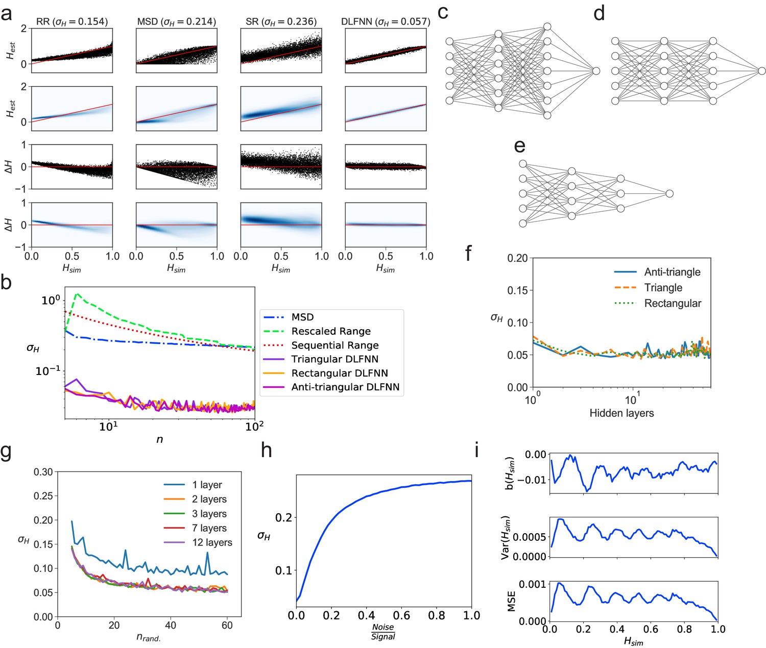
Tests of exponent estimation for the DLFNN using N = 10⁴ simulated fBm trajectories.

(a) Plots showing the Hurst exponent estimates of fBm trajectories with $n = 10^{2}$ data points by a triangular DLFNN with three hidden layers compared with conventional methods. Plots are vertically grouped by Hurst exponent estimation method: (left to right) rescaled range, MSD, sequential range and DLFNN. $σ_{H}$ values are shown in the title. *Top row*: Scatter plots of estimated Hurst exponents $H_{e s t}$ and the true value of Hurst exponents from simulation $H_{s i m}$ . The red line shows perfect estimation. *Second row*: Due to the density of points, a Gaussian kernel density estimation was made of the plots in the top row (see Materials and methods). *Third row*: Scatter plots of the difference between the true value of Hurst exponents from simulation and estimated Hurst exponent $Δ H = H_{s i m} - H_{e s t}$ . *Last row*: Gaussian kernel density estimation of the plots in the third row. (b) $σ_{H}$ as a function of the number of consecutive fBm trajectory data points $n$ for different methods of exponent estimation. Example structures for two hidden layers and $n = 5$ time series input points of the anti-triangular, rectangular and triangular DLFNN are shown in (**c, d** and e), respectively. (f) $σ_{H}$ as a function of the number of hidden layers in the DLFNN for triangular, rectangular and anti-triangular structures. (g) $σ_{H}$ as a function of the number of randomly sampled fBm trajectory data points $n_{r a n d}$ with different number of hidden layers in the DLFNN shown in the legend. (h) $σ_{H}$ as a function of the noise-to-signal ratio ( $\frac{N o i s e}{S i g n a l}$ ) (NSR) from Gaussian random numbers added to all $n = 10^{2}$ data points in simulated fBm trajectories. (i) Plots of bias $b (H_{s i m})$ , variance $Var (H_{s i m})$ and mean square error (MSE) as functions of $H_{s i m}$ . For each value of $H_{s i m}$ , fBm trajectories with $n = 100$ points were simulated and estimated by a triangular DLFNN.

Figure 2

Download asset Open asset

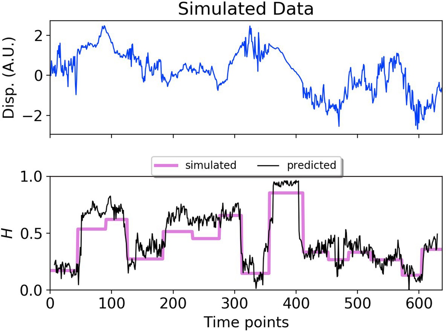
DLFNN analysis of a simulated trajectory.

*Top*: Plot of displacement as a function of time from a simulated fBm trajectory (blue) with multiple exponent values. *Bottom*: Hurst exponent values used for simulation (magenta), and the DLFNN exponent predictions of the neural network using a 15 point moving window (black).

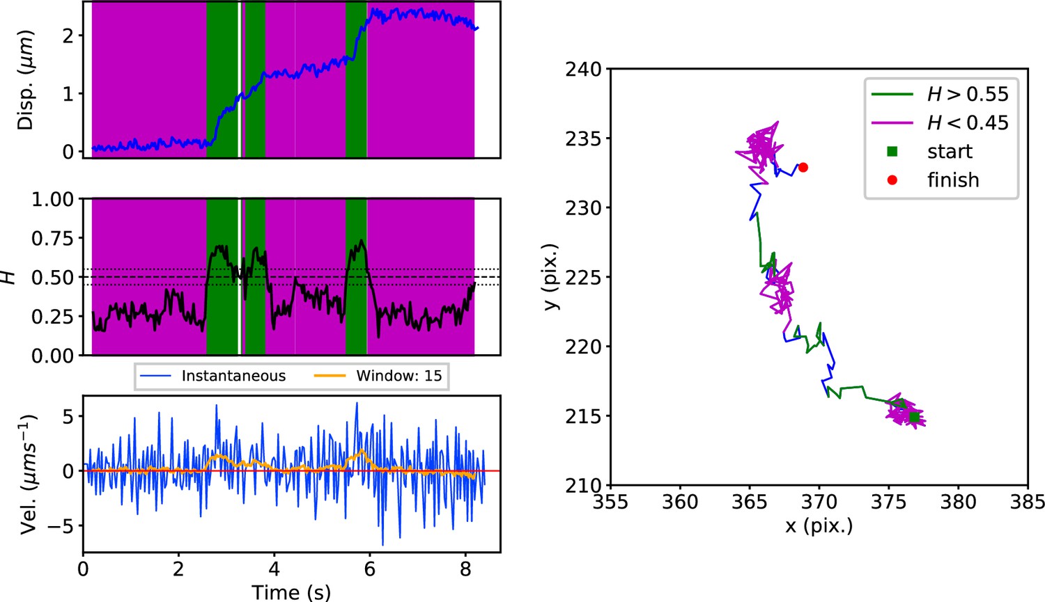
Figure 3 with 2 supplements

Download asset Open asset

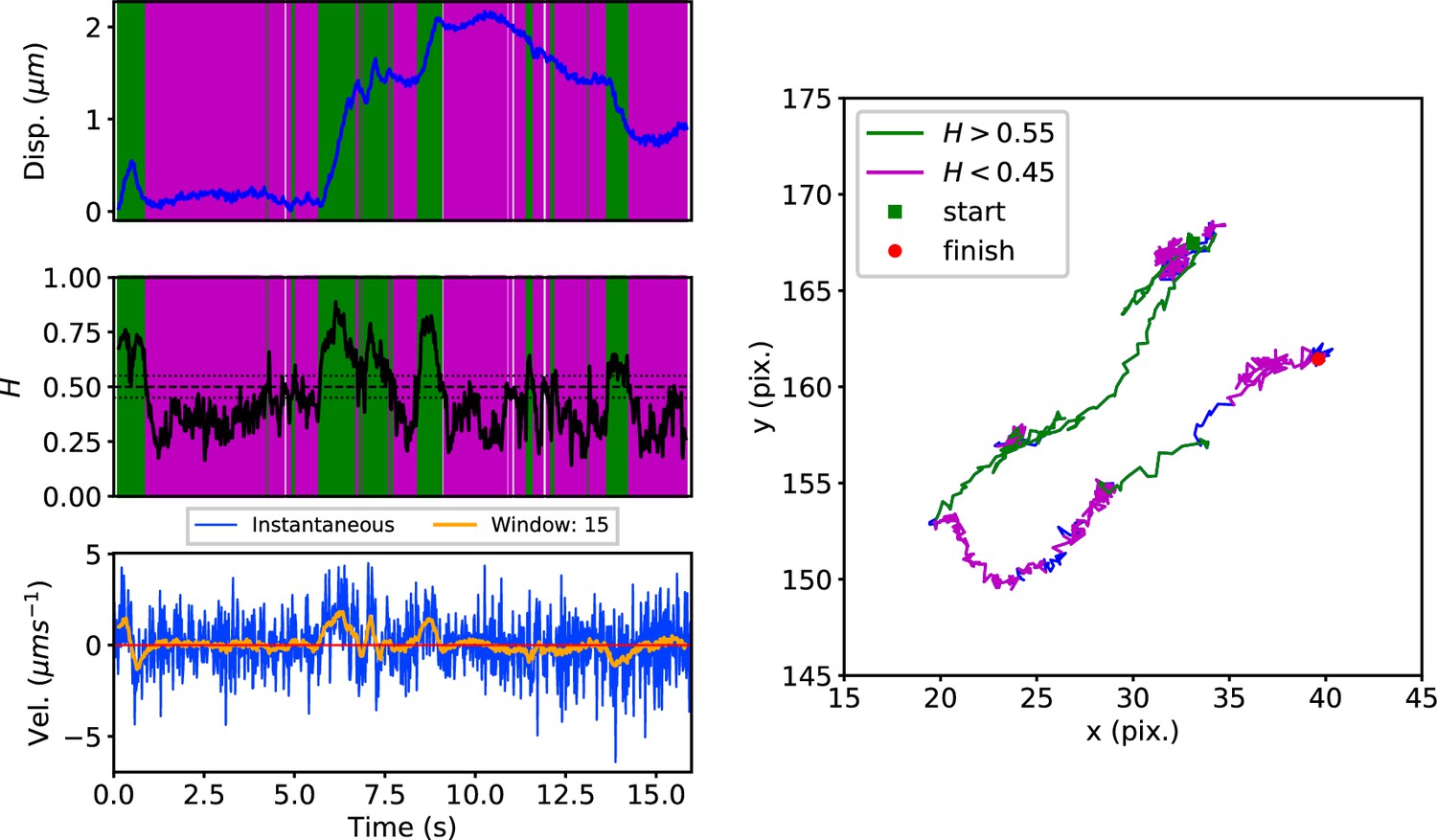
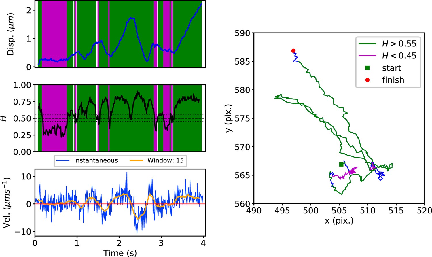
DLFNN analysis of a GFP-Rab5 endosome trajectory.

*Top*: Plot of displacement from a single trajectory in an MRC-5 cell (blue). Shaded areas show persistent (0.55 < H < 1 in green) and anti-persistent (0 < H < 0.45 in magenta) behaviour. *Middle*: A 15 point moving window DLFNN exponent estimate for the trajectory (black) with a line (dashed) marking diffusion H = 0.5 and two lines (dotted) marking confidence bounds for estimation marking H = 0.45 and 0.55. *Bottom*: Plot of instantaneous and moving (15 point) window velocity. *Right*: Plot of the trajectory with start and finish positions. Persistent (green) and anti-persistent (magenta) segments are shown. For sections that were 0.45 < H < 0.55 were not classified as persistent or anti-persistent and are depicted in blue.

Figure 3—figure supplement 1

Download asset Open asset

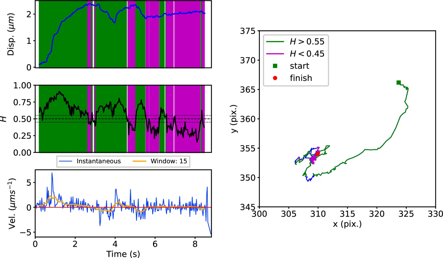
DLFNN analysis of a GFP-SNX1-labeled endosome trajectory, depicted as in Figure 3.

Figure 3—figure supplement 2

Download asset Open asset

DLFNN analysis of a lysosome trajectory, depicted as in Figure 3.

Figure 4

Download asset Open asset

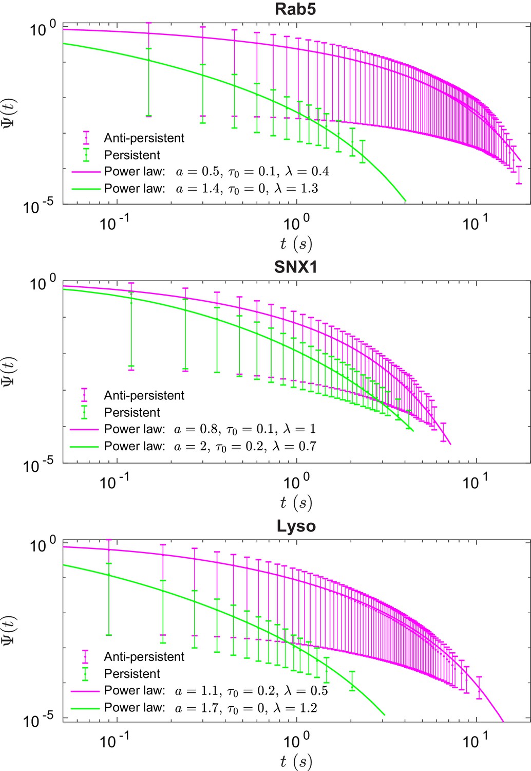
Survival functions plotted with error bars for persistent and anti-persistent segments for Rab5-positive endosomes, SNX1-positive endosomes and lysosomes with the power-law fits.

Fit parameters can be found in Appendix 3—table 1.

Figure 5

Download asset Open asset

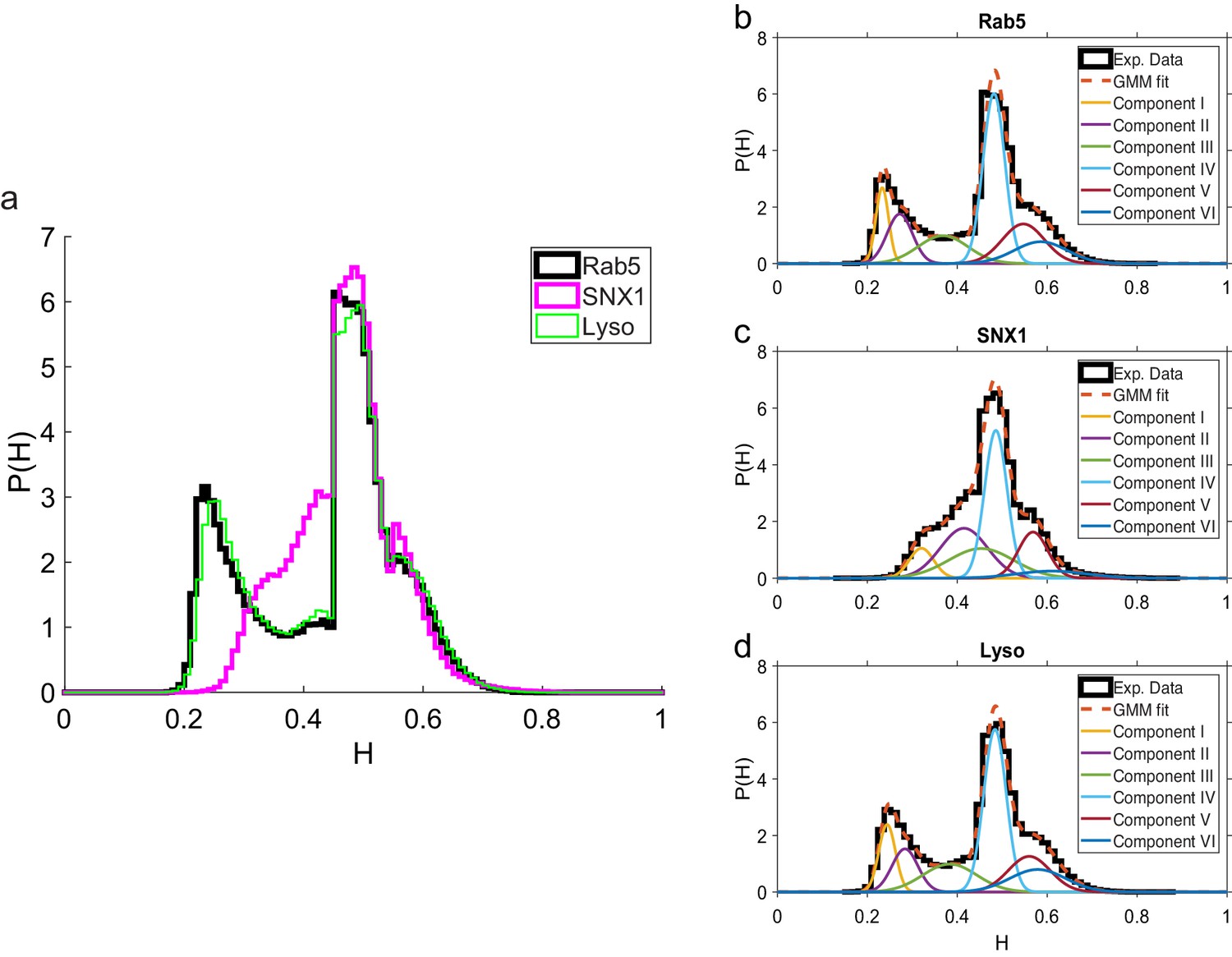
Comparison of Hurst exponent distributions for GFP-Rab5, GFP-SNX1 and lysosomes.

(a) Histograms of Hurst exponents for GFP-Rab5 (black), GFP-SNX1 (magenta) endosomes and lysosomes (green) plot on the same axes for comparison. The individual histograms of Hurst exponents (black solid) for GFP-Rab5-tagged endosomes, GFP-SNX1-tagged endosomes and lysosomes are shown in (**b, c** and d) respectively. For each histogram, the Gaussian mixture model fit for six components (red dashed) and individual Gaussian distribution components are shown on the same plot. The number of components were chosen through the Bayes information criterion shown in Appendix 4—figure 1.

Figure 6 with 4 supplements

Download asset Open asset

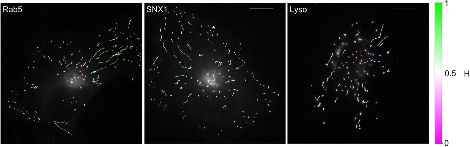
MRC-5 cells stably expressing GFP-Rab5, GFP-SNX1 or stained with Lysobrite with tracking data overlaid.

The colours show the value of $H$ estimated by the neural network using a 15 point window. The scalebar is 10 µm.

Figure 6—figure supplement 1

Download asset Open asset

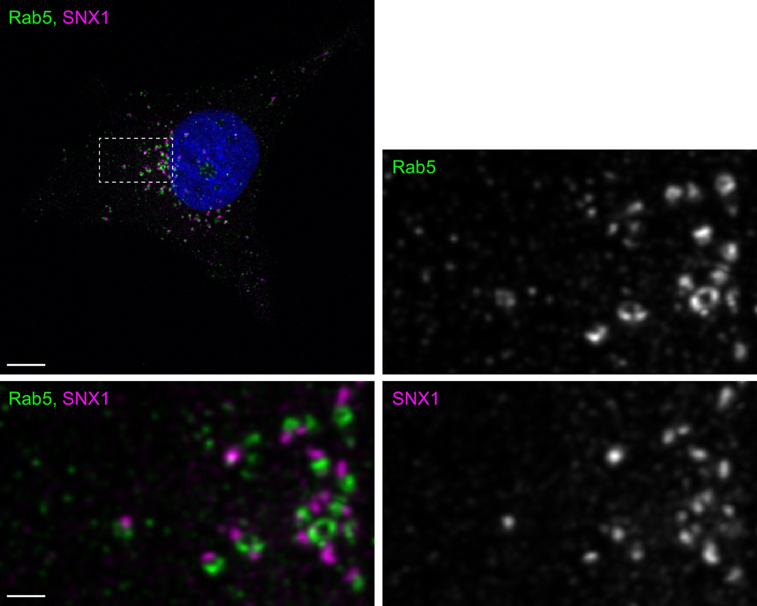
Distribution of endogenous Rab5 and SNX1.

MRC-5 cells were fixed and labeled with antibodies to Rab5 and SNX1, then imaged by confocal microscopy. A maximum-intensity z-projection of deconvolved images is shown. The boxed region is enlarged and presented as grey-scale single channels and a two color merged image. The scale bar is 10 µm (main image) and 2 µm (enlargements).

Figure 6—video 1

Download asset

posterframe for video — Video of MRC-5 cell stably expressing GFP-Rab5.

The field of view is 62.88 µm by 62.88 µm (600 × 600 pixels) and playback is in real time.

Figure 6—video 2

Download asset

Figure 6—video 3

Download asset

Figure 7

Download asset Open asset

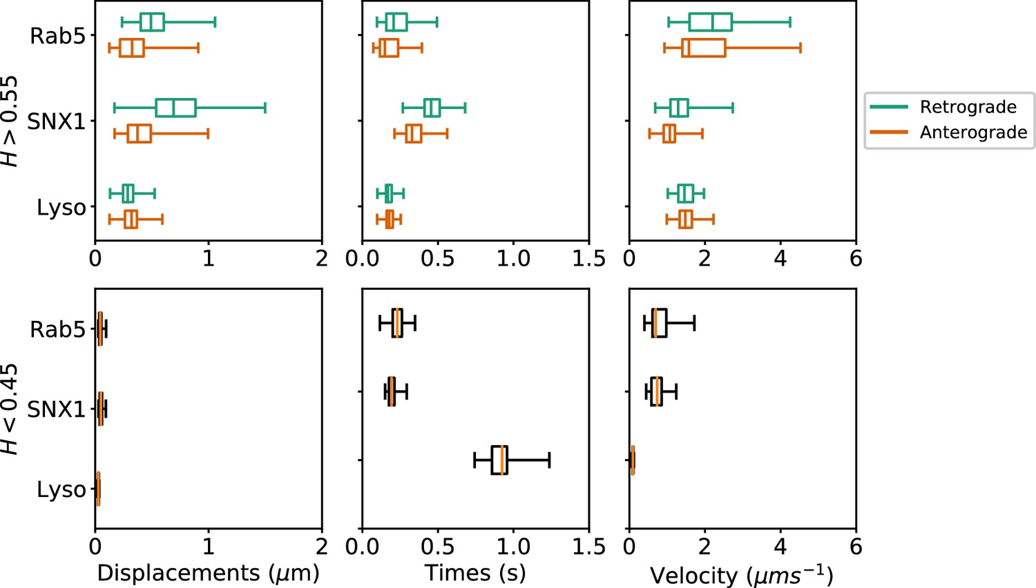
Box and whisker plots of displacements, times and velocities of persistent retrograde, persistent anterograde and anti-persistent segments in experimental trajectories.

Any segment with $H > 0.55$ was classed as persistent and $H < 0.45$ as anti-persistent. These H values were chosen as a precaution against the mean error of the neural network estimation. Each data point within the box and whisker plots are averages of all trajectory segments in a single cell. A total of 65 MRC-5 cells for GFP-Rab5-tagged endosomes, 63 MRC-5 cells for SNX1-GFP-tagged endosomes and 71 MRC-5 cells for lysosomes were analysed with at least 5 to 500 (average 54) anterograde or retrograde segments for each cell.

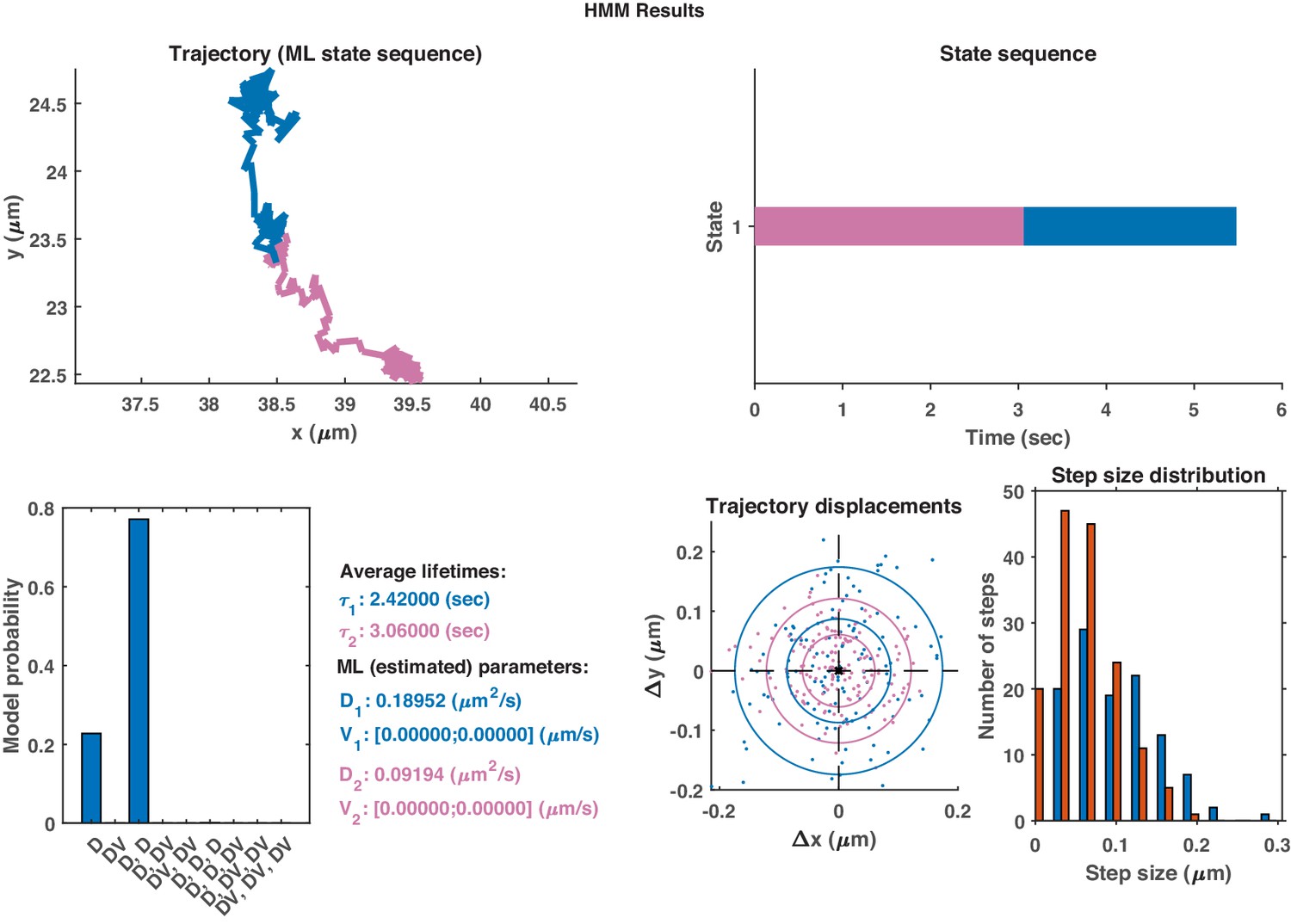
Appendix 1—figure 1

Download asset Open asset

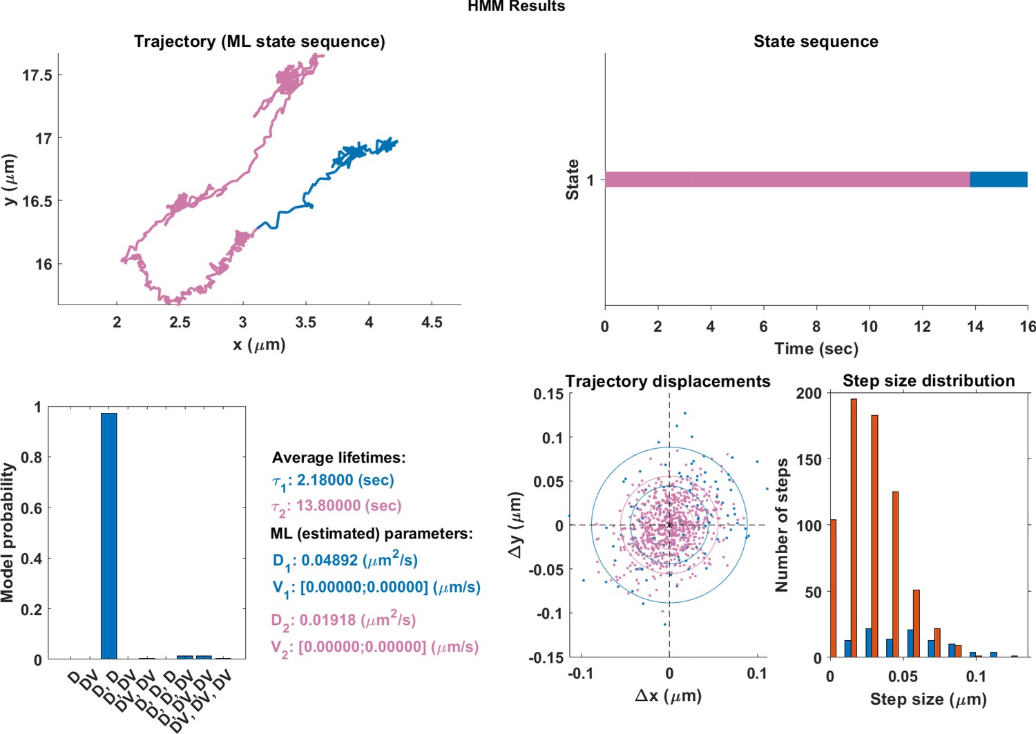
The same single trajectory as in Figure 3 but processed using the HMM-Bayes package described in Monnier et al. (2015).

The plot shows: the original trajectory (*top left*); the inferred state sequence of the most likely model (*top right*); the model probabilities given a maximum of three possible states (*bottom left*); the average lifetime of each state and estimated parameters of the most likely model (*bottom center left*), which in this case is two different diffusive states; individual increment displacements (*bottom center right*); and the step size distribution of those increments classed into the two different states.

Appendix 1—figure 2

Download asset Open asset

*Top*: Plot of displacement from a single GFP-SNX1 endosome trajectory in an MRC-5 cell (blue).

Shaded areas show persistent ( $0.55 < H < 1$ in green) and anti-persistent ( $0 < H < 0.45$ in magenta) behaviour. *Middle*: A 15 point moving window DLFNN exponent estimate for the trajectory (black) with a line (dashed) marking diffusion $H = 0.5$ and lines (dotted) marking the confidence bounds $H = 0.55$ and 0.45. *Bottom*: Plot of instantaneous and moving (15 point) window velocity. *Right*: Plot of the trajectory of a GFP-SNX1 endosome in an MRC-5 cell with start and finish positions, and persistent (green) and anti-persistent (magenta) segments indicated.

Appendix 1—figure 3

Download asset Open asset

The same HMM-Bayes analysis as shown in Appendix 1—figure 1 applied to the trajectory in Appendix 1—figure 2.

Appendix 2—figure 1

Download asset Open asset

Top: MSD (points) and power-law fits (dashed) for two different Brownian trajectories containing 1000 data points with diffusion coefficient 2.5 (red) and 0.025 (blue).

The Hurst exponent should be $α = 2 H = 1$ for both trajectories. Second Row: Simulation of the two Brownian trajectories with diffusion co-efficient 2.5 (red) and 0.025 (blue). Third Row: Local Hurst exponent estimates given by the DLFNN for the two different trajectories using a 90 point window. The averages of DLFNN Hurst exponent estimates are $α = 2 H = 1.110$ (red) and $α = 2 H = 1.114$ (blue). Bottom: Local Hurst exponent estimates of the $D = 2.5$ track given by DLFNN and MSDs using a 90 point window. The average of DLFNN Hurst exponent estimates is $α = 2 H = 1.110$ and the average of MSD estimates is $α = 2 H = 0.937$ .

Appendix 3—figure 1

Download asset Open asset

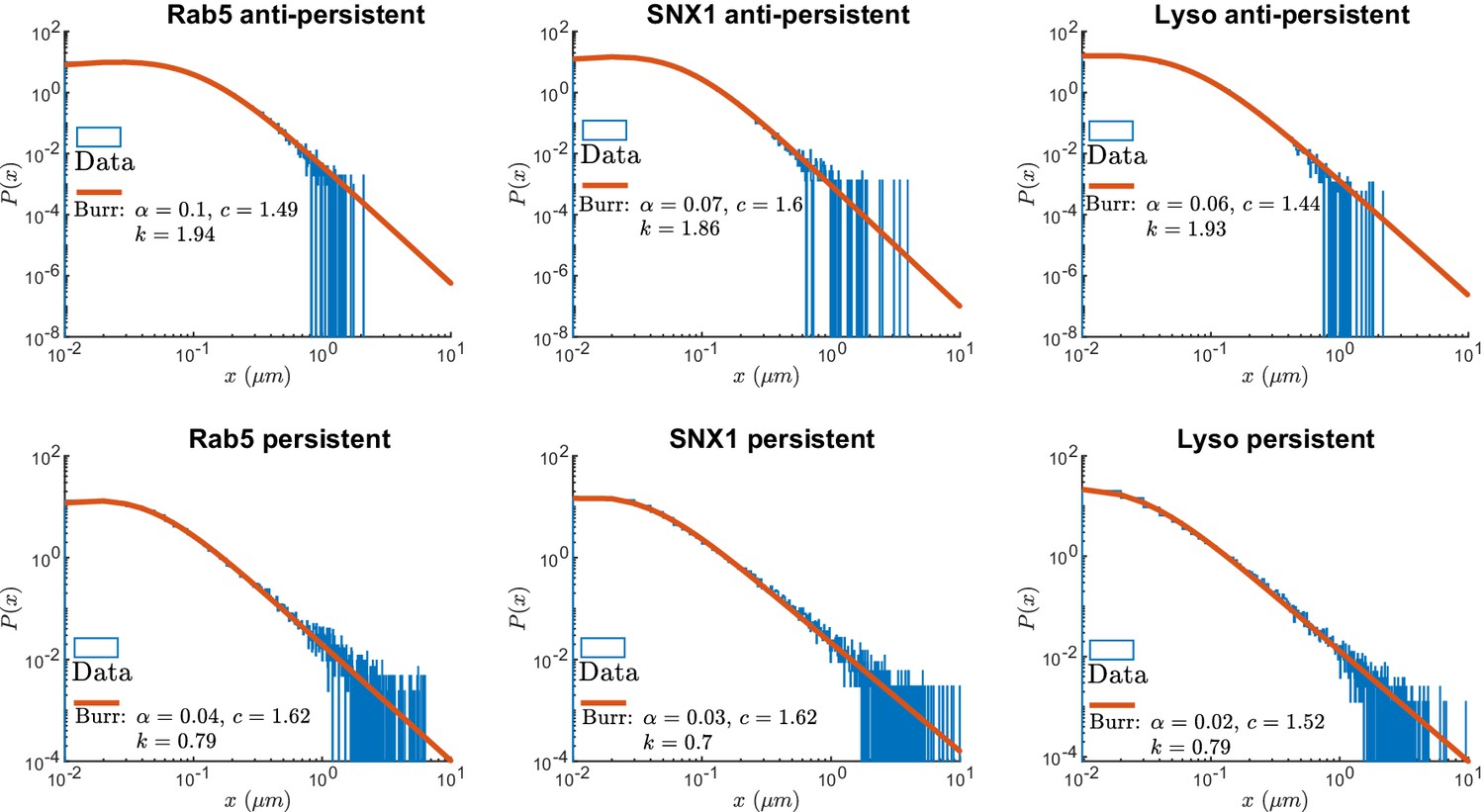
Normalized histograms (blue) and corresponding maximum likelihood estimation for Burr distributions (line) of segment displacements from lysosome and endosome experimental trajectories segmented using DLFNN.

Parameter estimates are shown the legend.

Appendix 4—figure 1

Download asset Open asset

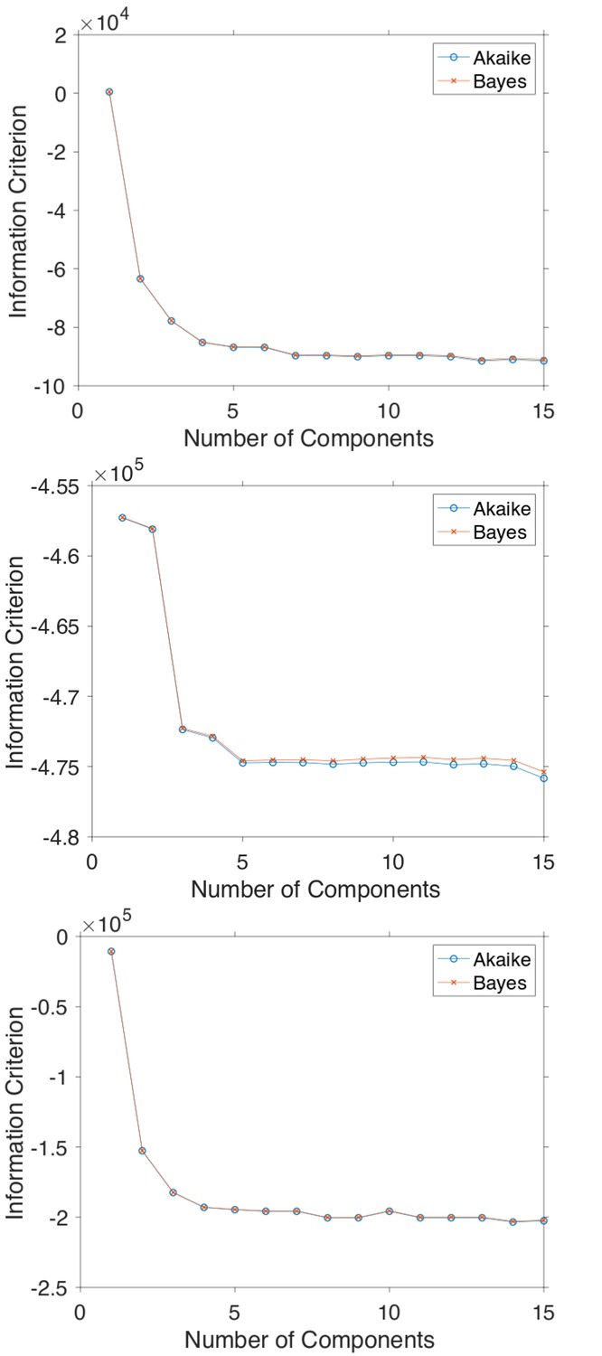
The Akaike and Bayes information criterion against number of components in the Gaussian mixture model shown in Figure 5 for GFP-Rab5 tagged endosomes (top), SNX1-GFP tagged endosomes (middle) and lysosomes (bottom).

Tables

Table 1

Statistics of experimental trajectory segments.

The persistent and anti-persistent segments in this table are: from trajectories that travelled over 0.5 µm at any point from their initial starting positions; contained more points than the window size; and switched behavior more than twice in the trajectory. Note that these conditions are much stricter than those to generate Figures 4 and 5. Each persistent segment was then further subdivided into retrograde and anterograde segments (see Materials and methods).

		Rab5	SNX1	Lyso
Number of persistent segments		2369	2099	7645
Number of anti-persistent segments		6983	3947	19,320
Number of retrograde segments		2925	2343	5882
Number of anterograde segments		2303	1609	6827
Anti-persistent displacement (µm)	Mean	0.05	0.05	0.03
	Median	0.04	0.05	0.03
	St. Dev	0.02	0.01	0.004
Anti-persistent speed (µms^-1)	Mean	0.82	0.75	0.10
	Median	0.70	0.73	0.09
	St. Dev	0.31	0.19	0.02
Anti-persistent time (s)	Mean	0.23	0.20	0.93
	Median	0.23	0.19	0.92
	St. Dev	0.05	0.03	0.11
Retrograde displacement (µm)	Mean	0.53	0.74	0.29
	Median	0.49	0.69	0.29
	St. Dev	0.19	0.28	0.08
Retrograde speed (µms^-1)	Mean	2.29	1.35	1.49
	Median	2.21	1.29	1.46
	St. Dev	0.87	0.39	0.25
Retrograde time (s)	Mean	0.22	0.46	0.17
	Median	0.21	0.45	0.17
	St. Dev	0.09	0.09	0.03
Anterograde displacement (µm)	Mean	0.35	0.43	0.31
	Median	0.33	0.37	0.32
	St. Dev	0.17	0.20	0.08
Anterograde speed (µms^-1)	Mean	2.06	1.10	1.51
	Median	1.71	1.08	1.48
	St. Dev	0.95	0.30	0.27
Anterograde time (s)	Mean	0.18	0.34	0.18
	Median	0.15	0.33	0.18
	St. Dev	0.08	0.08	0.03

Key resources table

Reagent type or resource	Designation	Source	Identifiers	Additional information
Cell line (Homo sapiens)	Lung fibroblast line	Allison et al., 2017 https://doi.org/10.1083/jcb.201609033	GFP-SNX1-MRC5	MRC5 cell line stably expressing GFP-SNX1. Mycoplasma free.
Cell line (H. sapiens)	Lung fibroblast line	Other	GFP-Rab5-MRC5	MRC5 cell line stably expressing GFP-Rab5 generated by retroviral transduction by G. Pearson and E. Reid, University of Cambridge. Mycoplasma free.
Cell line (H. sapiens)	MRC-5 SV1 TG1 Lung fibroblast line	ECACC	MRC-5 SV1 TG1 cells, cat no. 85042501	Mycoplasma free.
Antibody	Anti-human Rab5A Rabbit monoclonal	Cell Signalling Technology	3547S	IF(1/200)
Antibody	Anti-human sorting nexin 1 (mouse monoclonal)	BD Biosciences	611482	IF(1/200)
Antibody	Alexa594-conjugated anti-mouse IgG (donkey polyclonal)	Jackson ImmunoResearch	715-585-150	IF(1/400)
Antibody	A488-conjugated donkey anti-rabbit IgG	Jackson Immunoresearch	711-545-152	IF(1/400)
Recombinant DNA reagent	pLXIN-GFP-Rab5C-I-NeoR	Other		Used by G. Pearson and E. Reid, University of Cambridge to generate retrovirus containing GFP-Rab5C
Sequence-based reagent	Hpa1 GFP Forward	Other	PCR primer	Used by G. Pearson and E. Reid, University of Cambridge to generate retrovirus containing GFP-Rab5C. TAGGGAGTTAACATGGTGAGCAAGGGCGAGGA
Sequence-based reagent	Not1 Rab5C Reverse	Other	PCR primer	Used by G. Pearson and E. Reid, University of Cambridge to generate retrovirus containing GFP-Rab5C . ATCCCTGCGGCCGCTCAGTTGCTGCAGCACTGGC
Chemical compound, drug	DAPI	Biolegend	422801	IF (1 µg/mL)
Chemical compound, drug	Prolong Gold	ThermoFisher	P36930
Chemical compound, drug	Lysobrite Red	AAT Bioquest	22645	(1/2500)
Chemical compound, drug	Geneticin (G418)	Sigma-Aldrich	G1397	200 µg/mL to maintain GFP-Rab5-MRC5 and GFP-SNX1-MRC5 cells in culture.
Chemical compound, drug	Formaldehyde solution, 37% (wt/v)	Sigma-Aldrich	252549
Chemical compound, drug	Triton X-100	Anatrace	T1001
Software, algorithm	NNT (aitracker.net)	Newby et al., 2018	AITracker	Web-based automated tracking service
Software, algorithm	Metamorph	Molecular Devices LLC	Metamorph	Metamorph Microscopy Automation and Image Analysis Software
Software, algorithm	FIJI	Schindelin, J.; Arganda-Carreras, I. and Frise, E. et al. (2012) ,‘Fiji: an open-source platform for biological-image analysis’, Nature methods 9 (7): 676–682, PMID22743772, doi:10.1038/nmeth.2019	FIJI/ImageJ
Software, algorithm	DLFNN Exponent Estimator	Han, Daniel. (2020, January 20). DLFNN Exponent Estimator (Version 0). http://doi.org/10.1101/777615	DLFNN/DLFNN Exponent Estimator	Hurst exponent estimator with Deep Learning Feed-forward Neural Network application for Windows 10. Documentation included.
Software, algorithm	Python3	Python Software Foundation.Python Language Reference 3.7. Available at www.python.org	Python/Python3
Software, algorithm	SciPy	Virtanen et al. (2020) SciPy 1.0: Fundamental Algorithms for Scientific Computing in Python. Nature Methods, in press.	SciPy/scipy
Software, algorithm	Tensorflow	Abadi et al., 2016	Tensorflow
Software, algorithm	Keras	Chollet, François and others. ‘Keras.' (2015). Available from https://keras.io	Keras
Software, algorithm	fbm	Flynn, Christopher, fbm 0.3.0 available for download at https://pypi.org/project/fbm/ or https://github.com/crflynn/fbm	FBM package in Python	Exact methods for simulating fractional Brownian motion (fBm) or fractional Gaussian noise (fGn) in python. Approximate simulation of multifractional Brownian motion (mBm) or multifractional Gaussian noise (mGn).
Other	35 mm glass-bottomed dishes (µ-Dish)	Ibidi	Cat. No. 81150

Appendix 3—table 1

Results for the fits of survival time probabilities shown in Figure 4.

The parameters and the analytical survival functions used to fit the Kaplan-Meier estimator survival curves.

Rab5 data	Survival function $Ψ (t)$	Fit parameters for Figure 4
Anti-persistent	$e^{- λ t} {(\frac{τ_{0}}{τ_{0} + t})}^{μ}$	$μ = 0.518 \pm 0.004$ , $τ_{0} = 0.140 \pm 0.002 s$ , $λ = 0.352 \pm 0.002 s^{- 1}$
Persistent	$e^{- λ t} {(\frac{τ_{0}}{τ_{0} + t})}^{μ}$	$μ = 1.352 \pm 0.102$ , $τ_{0} = 0.045 \pm 0.006 s$ , $λ = 1.286 \pm 0.142 s^{- 1}$
SNX1 data	Survival function $Ψ (t)$	Fit parameters for Figure 4
Anti-persistent	$e^{- λ t} {(\frac{τ_{0}}{τ_{0} + t})}^{μ}$	$μ = 0.757 \pm 0.023$ , $τ_{0} = 0.118 \pm 0.006 s$ , $λ = 1.004 \pm 0.016 s^{- 1}$
Persistent	$e^{- λ t} {(\frac{τ_{0}}{τ_{0} + t})}^{μ}$	$μ = 2.034 \pm 0.205$ , $τ_{0} = 0.185 \pm 0.026 s$ , $λ = 0.659 \pm 0.137 s^{- 1}$
Lysosome data	Survival function $Ψ (t)$	Fit parameters for Figure 4
Anti-persistent	$e^{- λ t} {(\frac{τ_{0}}{τ_{0} + t})}^{μ}$	$μ = 1.113 \pm 0.009$ , $τ_{0} = 0.208 \pm 0.003 s$ , $λ = 0.5 s^{- 1}$ (fixed)
Persistent	$e^{- λ t} {(\frac{τ_{0}}{τ_{0} + t})}^{μ}$	$μ = 1.748 \pm 0.065$ , $τ_{0} = 0.041 \pm 0.003 s$ , $λ = 1.216 \pm 0.139 s^{- 1}$

Additional files

Transparent reporting form: https://cdn.elifesciences.org/articles/52224/elife-52224-transrepform-v3.pdf
Download elife-52224-transrepform-v3.pdf

Download links

A two-part list of links to download the article, or parts of the article, in various formats.

Downloads (link to download the article as PDF)

Open citations (links to open the citations from this article in various online reference manager services)

Mendeley

Cite this article (links to download the citations from this article in formats compatible with various reference manager tools)

Daniel Han
Nickolay Korabel
Runze Chen
Mark Johnston
Anna Gavrilova
Victoria J Allan
Sergei Fedotov
Thomas A Waigh

(2020)

Deciphering anomalous heterogeneous intracellular transport with neural networks

eLife 9:e52224.

https://doi.org/10.7554/eLife.52224

Figures

Tests of exponent estimation for the DLFNN using N = 10⁴ simulated fBm trajectories.

DLFNN analysis of a simulated trajectory.

DLFNN analysis of a GFP-Rab5 endosome trajectory.

DLFNN analysis of a GFP-SNX1-labeled endosome trajectory, depicted as in Figure 3.

DLFNN analysis of a lysosome trajectory, depicted as in Figure 3.

Survival functions plotted with error bars for persistent and anti-persistent segments for Rab5-positive endosomes, SNX1-positive endosomes and lysosomes with the power-law fits.

Comparison of Hurst exponent distributions for GFP-Rab5, GFP-SNX1 and lysosomes.

MRC-5 cells stably expressing GFP-Rab5, GFP-SNX1 or stained with Lysobrite with tracking data overlaid.

Distribution of endogenous Rab5 and SNX1.

Video of MRC-5 cell stably expressing GFP-Rab5.

Video of MRC-5 cell stably expressing GFP-SNX1.

Video of MRC-5 cell stained with Lysobrite.

Box and whisker plots of displacements, times and velocities of persistent retrograde, persistent anterograde and anti-persistent segments in experimental trajectories.

The same single trajectory as in Figure 3 but processed using the HMM-Bayes package described in Monnier et al. (2015).

Top: Plot of displacement from a single GFP-SNX1 endosome trajectory in an MRC-5 cell (blue).

The same HMM-Bayes analysis as shown in Appendix 1—figure 1 applied to the trajectory in Appendix 1—figure 2.

Top: MSD (points) and power-law fits (dashed) for two different Brownian trajectories containing 1000 data points with diffusion coefficient 2.5 (red) and 0.025 (blue).

Normalized histograms (blue) and corresponding maximum likelihood estimation for Burr distributions (line) of segment displacements from lysosome and endosome experimental trajectories segmented using DLFNN.

The Akaike and Bayes information criterion against number of components in the Gaussian mixture model shown in Figure 5 for GFP-Rab5 tagged endosomes (top), SNX1-GFP tagged endosomes (middle) and lysosomes (bottom).

Tables

Statistics of experimental trajectory segments.

Results for the fits of survival time probabilities shown in Figure 4.

Additional files

Transparent reporting form

Download links

Downloads (link to download the article as PDF)

Open citations (links to open the citations from this article in various online reference manager services)

Cite this article (links to download the citations from this article in formats compatible with various reference manager tools)

Be the first to read new articles from eLife

Share this article

Cite this article

Tests of exponent estimation for the DLFNN using N = 104 simulated fBm trajectories.

DLFNN analysis of a simulated trajectory.

DLFNN analysis of a GFP-Rab5 endosome trajectory.

DLFNN analysis of a GFP-SNX1-labeled endosome trajectory, depicted as in Figure 3.

DLFNN analysis of a lysosome trajectory, depicted as in Figure 3.

Survival functions plotted with error bars for persistent and anti-persistent segments for Rab5-positive endosomes, SNX1-positive endosomes and lysosomes with the power-law fits.

Comparison of Hurst exponent distributions for GFP-Rab5, GFP-SNX1 and lysosomes.

MRC-5 cells stably expressing GFP-Rab5, GFP-SNX1 or stained with Lysobrite with tracking data overlaid.

Distribution of endogenous Rab5 and SNX1.

Video of MRC-5 cell stably expressing GFP-Rab5.

Video of MRC-5 cell stably expressing GFP-SNX1.

Video of MRC-5 cell stained with Lysobrite.

Box and whisker plots of displacements, times and velocities of persistent retrograde, persistent anterograde and anti-persistent segments in experimental trajectories.

The same single trajectory as in Figure 3 but processed using the HMM-Bayes package described in Monnier et al. (2015).

Top: Plot of displacement from a single GFP-SNX1 endosome trajectory in an MRC-5 cell (blue).

The same HMM-Bayes analysis as shown in Appendix 1—figure 1 applied to the trajectory in Appendix 1—figure 2.

Top: MSD (points) and power-law fits (dashed) for two different Brownian trajectories containing 1000 data points with diffusion coefficient 2.5 (red) and 0.025 (blue).

Normalized histograms (blue) and corresponding maximum likelihood estimation for Burr distributions (line) of segment displacements from lysosome and endosome experimental trajectories segmented using DLFNN.

The Akaike and Bayes information criterion against number of components in the Gaussian mixture model shown in Figure 5 for GFP-Rab5 tagged endosomes (top), SNX1-GFP tagged endosomes (middle) and lysosomes (bottom).

Statistics of experimental trajectory segments.

Results for the fits of survival time probabilities shown in Figure 4.

Transparent reporting form

Downloads (link to download the article as PDF)

Open citations (links to open the citations from this article in various online reference manager services)

Cite this article (links to download the citations from this article in formats compatible with various reference manager tools)

Tests of exponent estimation for the DLFNN using N = 10⁴ simulated fBm trajectories.