Single-molecule turnover dynamics of actin and membrane coat proteins in clathrin-mediated endocytosis
- Yale University, United States
- Yale University School of Medicine, United States
Figures
Figure 1
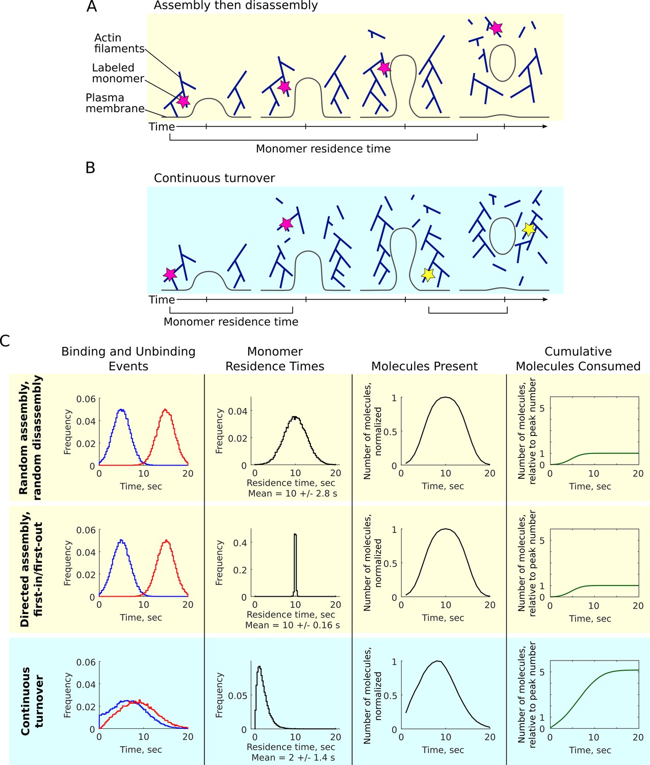
Different molecular mechanisms may give rise to similar apparent bulk dynamics.
(A–B) Many models suggest directed assembly and disassembly of actin in endocytosis but it is unclear whether the actin meshwork assembles and then disassembles in distinct phases (A) or continuously turns over during its bulk lifetime (B). Individual monomers are illustrated by magenta and yellow stars, with their residence times indicated. (C) Simulated assembly and disassembly according to different hypothetical models: random assembly and disassembly in separate phases (top row), directed assembly with first-in/first-out disassembly (middle row), assembly with continuous turnover (bottom row). Far left: simulated occurrences of binding (blue) and unbinding events (red) underlying the assembly and disassembly mechanisms. Mid left: residence times of individual molecules, a quantity that clearly differentiates between the models. Mid right: number of molecules over time, a measurable quantity that can appear similar across the models. Far right: cumulative number of molecules consumed over time, normalized to the peak number of molecules present.
Figure 2 with 9 supplements

Endocytic protein lifetimes assessed by patch tracking, FRAP, and single-molecule tracking.
(A) Sum intensity projection image of 10 frames (1 s) from a movie of cells expressing Acp1p-mEGFP (heterodimeric actin capping protein subunit) imaged in partial-TIRF (Figure 2—video 1), inverted contrast. Scale bar is 5 µm. (B) Montage of GFP spot, shown at 1 s increments, with the lifetime of the spot indicated by the green bar above the image panels. Right: trajectory of a spot, color-coded with blue at the start and red at the end. Scale bars are 1 µm. (C) Distribution of Acp1p-mEGFP patch lifetimes, as measured by semi-automatic tracking with TrackMate. N = 51 tracks from five movies recorded in two independent samples. (D) Acp1p-mEGFP cells were imaged by scanning confocal microscope to record fluorescence recovery after photobleaching of localized regions (Figure 2—video 5). Kymographs (above) and background-subtracted fluorescence intensity over time (below) for Acp1p-mEGFP patches (gap in kymograph and intensity spans three or ten frames of localized photobleaching; the unbleached patch is outside of the bleached region but no images are recorded during bleaching). Left: unbleached patch. Right: photobleached patch rapidly recovers to pre-bleached intensity (~1 s) and continues to develop to peak intensity comparable to unbleached patch. Green bar indicates photobleaching pulse. (E) Sum projection image of 10 frames (1 s) from a movie of cells expressing Acp1p-SNAP and sparsely labeled with SNAP-SiR imaged in partial-TIRF, inverted contrast (Figure 2—video 6). Scale bar is 5 µm. (F) Montage of SNAP+SiR spots, shown at 0.2 s increments. Trajectories shown at right (as in C), with scale bars 1 µm. (G) Distribution of Acp1p-SiR spot lifetimes, as measured by single-molecule localization and tracking with PYME. N = 4977 tracks from 24 movies recorded in five independent samples. Panels A-B and E-F have been prepared with different brightness settings for visual clarity. See Figure 2—video 1 and Figure 2—video 5 for example raw data.
Figure 2—figure supplement 1
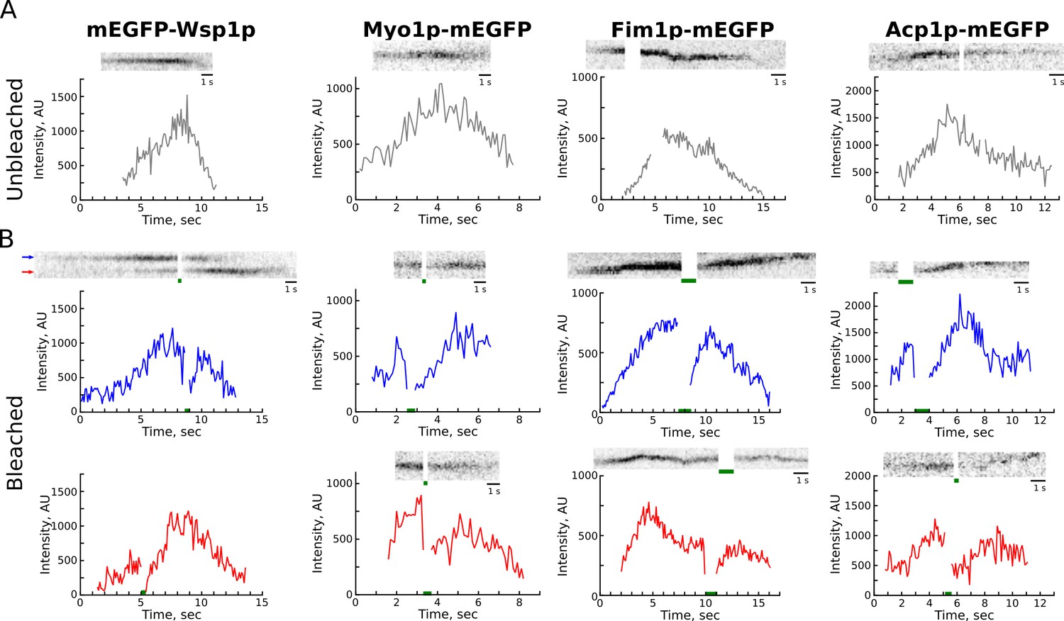
Fluorescence recovery after photobleaching of endocytic proteins.
(A) Kymographs (above) and background-subtracted fluorescence intensity over time (below) for mEGFP patches of actin nucleation-promoting factor Wsp1p (Figure 2—video 2), myosin-I Myo1p (Figure 2—video 3), actin crosslinker Fim1p (Figure 2—video 4), and heterodimeric actin capping protein subunit Acp1p (Figure 2—video 5). The gap in kymograph and intensity spans three or ten frames of localized photobleaching. (B) Kymographs (above) and background-subtracted fluorescence intensity over time (below) for four endocytic proteins of interest (as in A) targeted for localized photobleaching. Photobleached patches rapidly recover to pre-bleached intensity (~1–2 s) and continue to develop to peak intensity comparable to unbleached patch. Green bar indicates photobleaching pulse.
Figure 2—figure supplement 2

Characterization of SNAP-tag labeling.
(A) S. pombe cells expressing Fim1p-mEGFP imaged in TIRF with 488 nm excitation (upper: bright-field image, lower: GFP emission). (B–C) Fim1p-SNAP cells (B, Figure 3—video 1) and wild-type cells (C, Figure 2—video 7) were incubated with 1 μM SNAP-SiR overnight and imaged in TIRF with 642 nm excitation (upper: bright-field image, lower: SiR emission). (D) Cells co-expressing Fim1p-SNAP and Acp2p-mEGFP were labeled with 1 μM SNAP-SiR overnight and imaged in bright-field (upper left), SiR channel (middle left), GFP channel (lower left), and overlaid (right) to assess colocalization of single-molecule Fim1p-SiR spots with endocytic patches. (E) Average number of spots visible in initial frames of movies of Fim1p-mEGFP (as in A), Acp2p-mEGFP (as in D) or Fim1p-SiR (as in B and D), and wild-type cells (as in C). At least three images were analyzed for each sample, manually counting patches in 50 to 60 cells; for wild-type cells five images containing 591 cells were analyzed with spot localization and tracking thresholds as described in the text. Cell outlines are drawn in orange dash for fluorescence images. Scale bars for A-D are 5 μm.
Figure 2—video 1
Acp1-mEGFP The movie was recorded at 10 frames per second and is shown as inverted contrast.
Figure 2—video 2
FRAP of mEGFP-Wsp1p The movie was recorded at 10 frames per second and is shown as inverted contrast.
The blue box represents the region that was bleached every 10 s for 300 ms. The frames of the movie when photobleaching was performed are blank.
Figure 2—video 3
FRAP of mEGFP-Myo1p The movie was recorded at 10 frames per second and is shown as inverted contrast.
The blue box represents the region that was bleached every 10 s for 300 ms. The frames of the movie when photobleaching was performed are blank.
Figure 2—video 4
FRAP of Fim1p-mEGFP The movie was recorded at 10 frames per second and is shown as inverted contrast.
The blue box represents the region that was bleached every 10 s for 1000 ms. The frames of the movie when photobleaching was performed are blank.
Figure 2—video 5
FRAP of Acp1p-mEGFP The movie was recorded at 10 frames per second and is shown as inverted contrast.
The blue box represents the region that was bleached every 10 s for 300 ms. The frames of the movie when photobleaching was performed are blank.
Figure 2—video 6
Acp1-SNAP+SiR The movie was recorded at 10 frames per second and is shown as inverted contrast.
Figure 2—video 7
Wild type (FY527) + SiR The movie was recorded at 10 frames per second and is shown as inverted contrast.
Figure 3 with 14 supplements
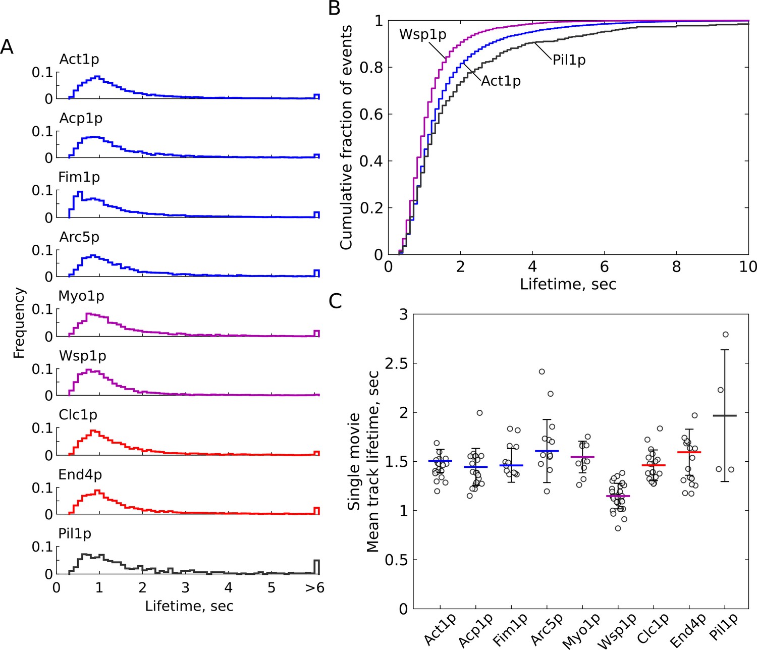
Single-molecule residence times of several endocytic proteins.
Cells expressing SNAP-tag fusion proteins were sparsely labeled with SiR-647 then imaged and tracked as described in text. (A) Probability distributions of track lifetimes for each target protein. Distributions are truncated at 6 s and all events longer than 6 s are shown in the final bin. The minimum allowed track length is 0.3 s. (B) Cumulative distributions of Act1p (blue), Wsp1p (purple) and Pil1p (gray). (C) Mean track lifetimes calculated for each movie and standard deviation (calculated across means of all images with more than 40 tracks), individual dataset means shown by open circles. See Table 2 for summary statistics. Actin-associated endocytic proteins are colored in blue, nucleation-promoting factors are purple, and membrane-associated endocytic proteins are red. Pil1p is included as an ‘immobile’ control in gray, although the detected tracks represent a mixture of stable molecules incorporated in eisosomes and dynamic molecules at eisosome ends. Figure 2—videos 6, 7, Figure 3—videos 1, 2, 3, 4, 5, 6, 7 are representative movies from which the data shown in this figure have been extracted.
Figure 3—figure supplement 1
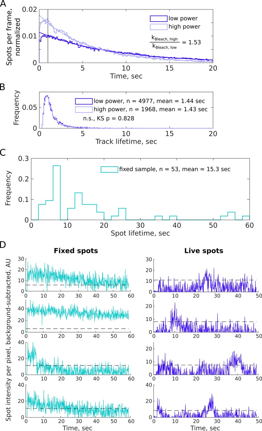
Photobleaching does not affect single-molecule track lifetimes.
(A) The number of spots across all movies decreases over time due to photobleaching. Acp1p-SiR labeled samples were imaged at two laser powers. Dark and light curves indicate illumination at 0.5 (Figure 2—video 6) and 0.8 W/cm2 (Figure 3—video 8), or a 1.6-fold increase in power. The total number of spots per frame is fit with an exponential decay, excluding early time bins (t < 1 s, black line) which are under-populated due to image crowding or high background signal. The decay rates for the fitted curves at low and high power are 0.12 and 0.18 sec−1, a relative difference of 1.53-fold. (B) Track lifetimes for Acp1p-SiR, from images recorded at low (Figure 2—video 6) and high (Figure 3—video 8) laser power (dark and light curves, respectively). Each dataset is taken from at least ten total images recorded in two samples. (C) Lifetimes of spots observed in Acp1p-SiR sample after fixation with formaldehyde, imaged under the same conditions used for tracking datasets, 0.5 W/cm2 illumination in partial-TIRF and recorded under identical camera exposure and frame acquisition time (100 msec per frame) (Figure 3—video 9). Fluorescent spots in fixed samples were manually tracked with FIJI/ImageJ TrackMate plugin. (D) Spot intensity for representative single-molecule fluorescence events in fixed (left) or live (right) cells expressing Acp1p-SNAP+SiR, imaged under identical illumination and camera settings, 100 msec per frame. Spot intensity in each frame was measured in Fiji for a 4-pixel diameter circle and the value of a nearby cytoplasmic region was subtracted as background. The spot intensity is plotted as solid line (teal or blue) and the background region’s standard deviation over the recording time is plotted as dashed line. Note that the intensity values shown here are calculated with methods unrelated to the methods used for spot tracking and lifetime analyses.
Figure 3—figure supplement 2
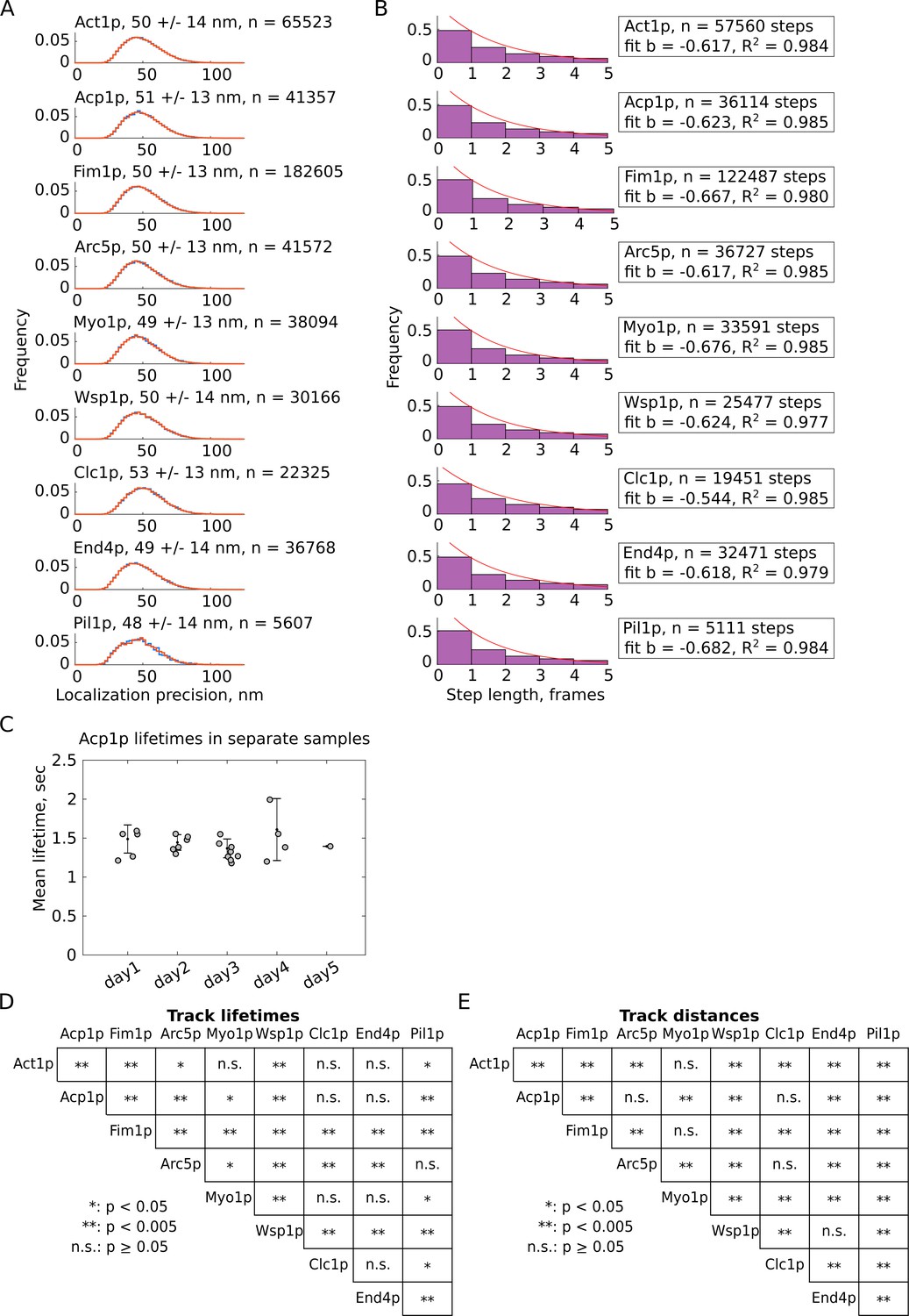
Characterization of single-molecule localization and tracking data.
(A) Distribution of spot localization precision in X (blue) and Y position (orange) for all tracks in each target protein dataset. Mean, standard deviation and number of points are given above each plot. (B) Distribution of track linking gap times, with single exponential fit curves. Fit curve decay rate and R2 values are given in the legends. (C) Variance between five independent samples of Ac1p-SiR lifetimes. Mean lifetimes (gray circles) and standard deviation (error bars) of each day’s datasets. (D) Statistical significance of differences between lifetimes distributions by Mann-Whitney test (full distributions shown in Figure 3A). (E) Statistical significance of differences between distributions of track displacements by Mann-Whitney test (full distributions shown in Figure 4A).
Figure 3—figure supplement 3
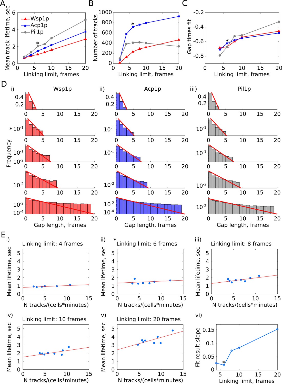
Effects of varying tracking gap-linking parameter.
A subset of images was processed with varying track linking limit parameter, that is the maximum number of frames spanning a gap where a spot is not detected. For linking limit of 6, the longest allowed time step is five frames, or four missed detections. (A) Dependence of average track lifetimes on the track gap-linking limit parameter. (B) Dependence of the number of detected tracks with track gap-linking limit. (C) Exponential decay rates of gap time distributions for each protein with varying track gap-linking limit. (D) Gap time distributions for tracks resulting from increasing gap-linking limit for Wsp1p (i), Acp1p (ii), and Pil1p (iii). Top to bottom: linking limit 4, 6, 8, 10, and 20. Single exponential curves are fitted for each and drawn in red. Plots are shown with log Y scale. (E) Dependence of mean track lifetime on label density. The same eight images of Acp1p-SiR were analyzed with varying gap-linking limit. The average number of tracks per cell per minute was used as a proxy for labeling efficiency. If fewer than 40 tracks were detected in an image, the values were not included. Datasets with linking limit two were omitted from (D) and (E) because there are too few resulting tracks. *: Linking limit of 6 frames was used for further analysis.
Figure 3—figure supplement 4
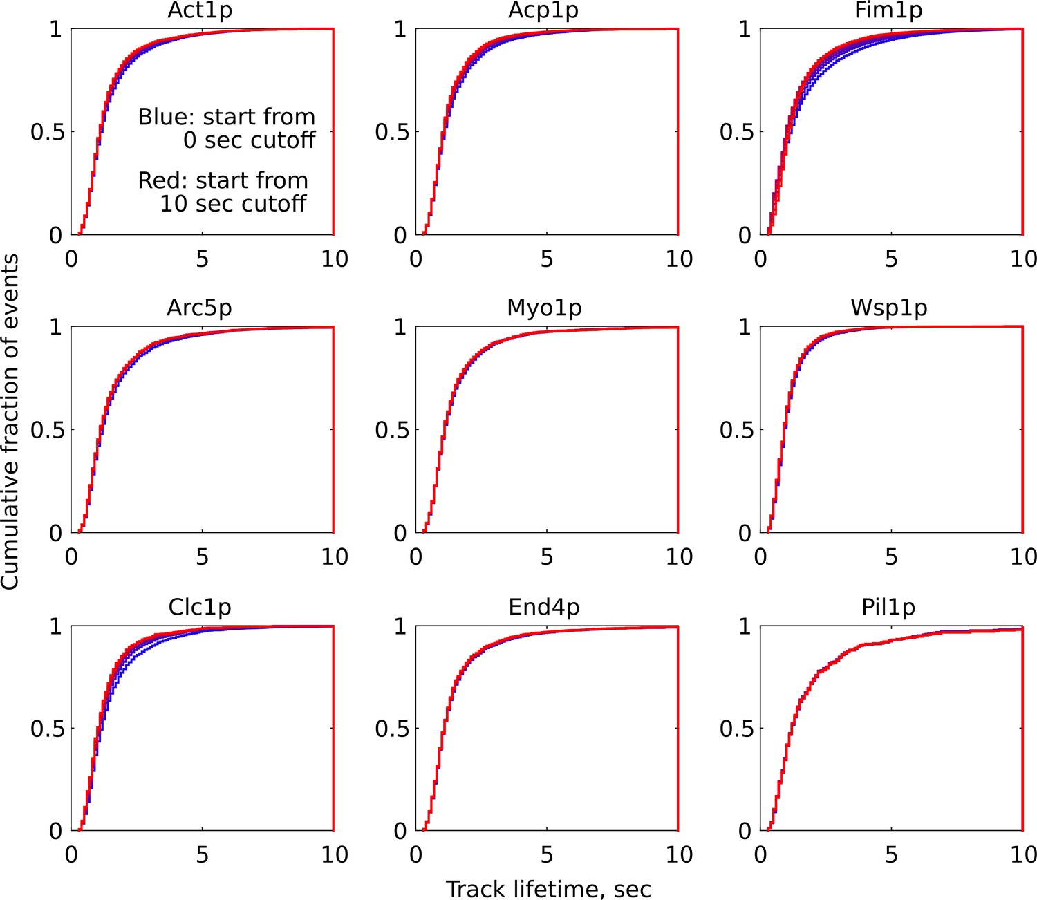
Dependence of track lifetimes on illumination start time cutoff.
Tracks were excluded from lifetime distribution by varying the start time cutoff in 1 s increments. The blue curve represents all track lifetimes from the absolute start of the movie, and curves of increasing red color include only tracks that start after the designated cutoff time. Some proteins show no significant shift in lifetimes distribution over time (e.g. Myo1p or End4p), while other proteins show clearly that the early tracks include significantly longer tracks (e.g. Act1p, Acp1p, Fim1p, Clc1p). Pil1p tracks were already analyzed beginning after 20 s of illumination and so further cutoffs have no effect.
Figure 3—video 1
Act1p-SNAP+SiR The movie was recorded at 10 frames per second and is shown as inverted contrast.
Figure 3—video 2
Fim1p-SNAP+SiR The movie was recorded at 10 frames per second and is shown as inverted contrast.
Figure 3—video 3
Arc5p-SNAP+SiR The movie was recorded at 10 frames per second and is shown as inverted contrast.
Figure 3—video 4
SNAP-Myo1p+SiR The movie was recorded at 10 frames per second and is shown as inverted contrast.
Figure 3—video 5
SNAP-Wsp1p+SiR The movie was recorded at 10 frames per second and is shown as inverted contrast.
Figure 3—video 6
Clc1p-SNAP+SiR The movie was recorded at 10 frames per second and is shown as inverted contrast.
Figure 3—video 7
End4p-SNAP+SiR The movie was recorded at 10 frames per second and is shown as inverted contrast.
Figure 3—video 8
Pil1p-SNAP+SiR The movie was recorded at 10 frames per second and is shown as inverted contrast.
Figure 3—video 9
Acp1p-SNAP+SiR, high laser power The movie was recorded at 10 frames per second and is shown as inverted contrast.
Figure 3—video 10
Acp1-SNAP+SiR, fixed cells The movie was recorded at 10 frames per second and is shown as inverted contrast.
SuppFile1lifetimes_simulator.m - Matlab simulation script for modeling assembly and disassembly profiles to illustrate the logic of ‘turnover’.
Figure 4
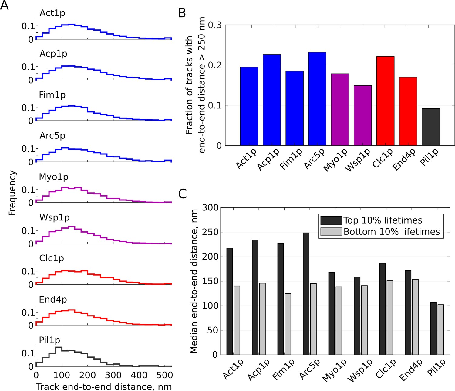
Single-molecule tracks net distances.
(A) Distributions of end-to-end distances for tracks of SNAP-tag fusion proteins. Actin-associated endocytic proteins are shown in blue, nucleation-promoting factors in purple, membrane-associated endocytic proteins in red, Pil1p as an ‘immobile’ control in gray. (B) Fraction of tracks with end-to-end distance longer than 250 nm for each sample. Colors as in (A). (C) Median distances of tracks in the top or bottom 10% of lifetime distributions for each sample. Figure 2—videos 6, 7, Figure 3—videos 1, 2, 3, 4, 5, 6, 7 are representative movies from which the data shown in this figure have been extracted.
Figure 5
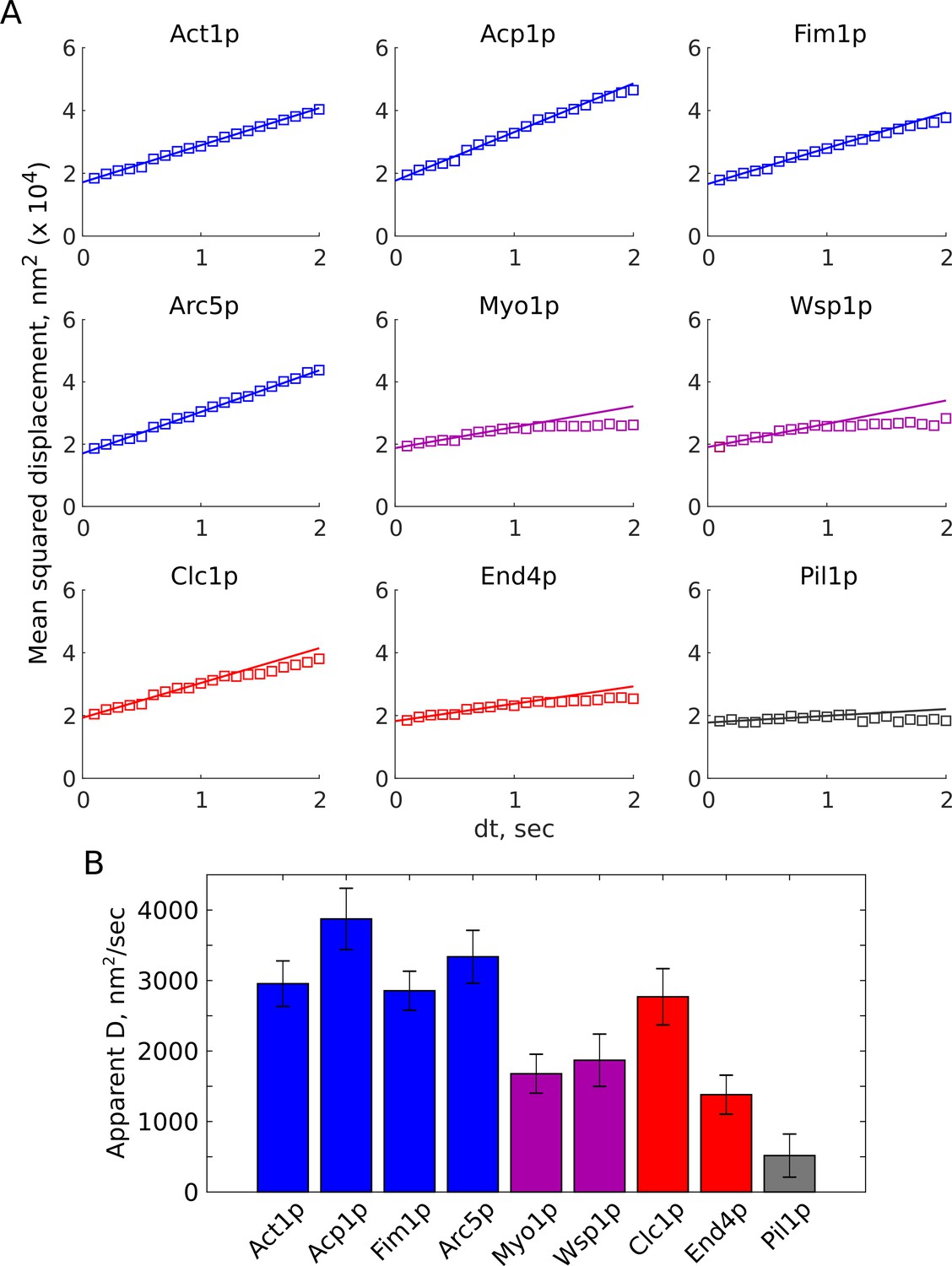
Average motions of endocytic proteins.
(A) Mean squared-displacement over time, computed across all pairwise distances in all tracks (squares), with their linear fits (solid lines). (B) Apparent diffusion coefficients (D) for analyzed proteins, assuming 2-dimensional diffusion, MSD = 4D*dt + b. Error bars show the 95% confidence interval associated with the fit of MSD vs. dt slope. Actin-associated endocytic proteins are shown in blue, nucleation-promoting factors in purple, membrane-associated endocytic proteins in red, Pil1p as an ‘immobile’ control in gray. Figure 2—videos 6, 7, Figure 3—videos 1, 2, 3, 4, 5, 6, 7 are representative movies from which the data shown in this figure have been extracted.
Figure 6

Distributions of single-molecule motions of endocytic proteins.
(A) Pairwise distances over time calculated for all pairs of points in each track show a range of mobility behaviors. Contour lines represent 3D histogram bins of identical height, normalized by the total number of points in each dataset, with relative density (arbitrary scaling units as indicated in the first panel). The mean displacements over time (heavy black line) and standard deviation (thin black lines) are shown for each time step shorter than 10 s. The plots are divided into high-, mid-, and low-mobility zones as indicated by black dotted lines. (B) The fractions of all pairwise displacements from (A) that fall into high-, mid-, and low-mobility classes for each dataset. Figure 2—videos 6, 7, Figure 3—videos 1, 2, 3, 4, 5, 6, 7 are representative movies from which the data shown in this figure have been extracted.
Tables
Table 1
Statistics for tracking of Acp1p-mEGFP endocytic patches.
| Name | Median, sec | Mean, sec | S.D., sec* | 95%ile, sec | N tracks | N samples |
|---|---|---|---|---|---|---|
| Acp1-mEGFP | 18.6 | 18.4 | 3.5 | 22.7 | 51 | 2 |
-
*Standard Deviation is calculated for the distribution of track lifetimes.
Table 2
Statistics for single-molecule tracks of SNAP-tag fusion proteins.
| Name | Lifetime Median, sec | Lifetime Mean, sec | Lifetime S.D., sec* | Lifetime 95%ile, sec | End-to-end distance Median, nm | n tracks | N movies (datasets with > 40 tracks) | N samples | D, nm2/sec † |
|---|---|---|---|---|---|---|---|---|---|
| Act1p | 1.1 | 1.5 | 0.12 | 4 | 159 | 7660 | 18 (18) | 2 | 2955 |
| Acp1p | 1.1 | 1.4 | 0.19 | 3.6 | 167 | 4977 | 24 (21) | 5 | 3874 |
| Fim1p | 1 | 1.5 | 0.17 | 4.2 | 154 | 16,490 | 12 (12) | 2 | 2855 |
| Arc5p | 1.2 | 1.6 | 0.32 | 4.2 | 166 | 4576 | 17 (13) | 2 | 3337 |
| Myo1p | 1.1 | 1.6 | 0.16 | 3.9 | 156 | 3951 | 10 (10) | 2 | 1678 |
| Wsp1p | 0.9 | 1.2 | 0.13 | 2.6 | 147 | 4379 | 41 (32) | 5 | 1869 |
| Clc1p | 1.1 | 1.5 | 0.16 | 3.7 | 168 | 2718 | 19 (18) | 3 | 2770 |
| End4p | 1.1 | 1.6 | 0.24 | 4.1 | 148 | 3983 | 31 (17) | 5 | 1381 |
| Pil1p | 1.2 | 2.0 | 0.67 | 5.9 | 134 | 446 | 6 (4) | 1 | 517 |
-
*Standard Deviation is determined across means calculated from individual datasets (each movie), only counting movies with >40 tracks.
†Apparent diffusion coefficient calculated from mean squared-displacement over time for time windows < 1 s (10 points), as in Figure 5.
Table 3
Statistics for single-molecule tracks of SNAP-tag fusion proteins imaged under alternate conditions.
| Name | Median, sec | Mean, sec | S.D., sec * | 95%ile, sec | N tracks | N movies (datasets with > 40 tracks) | N samples | D, nm2/sec † |
|---|---|---|---|---|---|---|---|---|
| Acp1p [high laser power] | 1.1 | 1.43 | 0.12 | 3.7 | 1968 | 11 (11) | 2 | 3367 |
| Acp1p [fixed]‡ | 12.0 | 15.3 | n.d. | 54.1 | 53 | 6 | 1 | n.d. |
-
* Standard Deviation is determined across means calculated from individual datasets (each movie), only counting movies with >40 tracks.
† Apparent diffusion coefficient calculated from mean squared-displacement over time for time windows < 1 s (10 points).
-
‡ Acp1p-SiR sample fixed with formaldehyde and imaged under the same illumination conditions (low power) and camera settings as live samples (Table 2).
Key resources table
| Reagent type (species) or resource | Designation | Source or reference | Identifiers | Additional information |
|---|---|---|---|---|
| Strain, strain background (Schizosaccharomyces pombe) | Wild-type | S Forsburg | FY527 | ade6-M216 his3-D1 leu1-32 ura4-D18 h- |
| Strain, strain background (S. pombe) | Fim1p-SNAP | This study | JB135 | fim1-SNAP-kanMX6 ade6-M216 his3-D1 leu1-32 ura4-D18 h- |
| Strain, strain background (S. pombe) | Acp2p-mEGFP/Fim1p-SNAP | This study | JB150 | acp2-mEGFP-kanMX6 fim1-SNAP-kanMX6 ade6-M216 his3-D1 leu1-32 ura4-D18 h- |
| Strain, strain background (S. pombe) | Pil1p-SNAP | (Lacy et al., 2017) | JB198 | pil1-SNAP-kanMX6 ade6-M216 his3-D1 leu1-32 ura4-D18 h- |
| Strain, strain background (S. pombe) | Clc1p-SNAP | This study | JB202 | clc1-SNAP-kanMX6 ade6-M216 his3-D1 leu1-32 ura4-D18 h- |
| Strain, strain background (S. pombe) | SNAP-Act1p | This study | JB216 | 41nmt1-SNAP-actin-leu+ ade6-M216 his3-D1 ura4-D19 h- |
| Strain, strain background (S. pombe) | SNAP-Myo1p | This study | JB304 | SNAP-myo1 fex1Δ fex2Δ ade6-M216 his3-D1 leu1-32 ura4-D18 h- |
| Strain, strain background (S. pombe) | Acp1p-SNAP | This study | JB305 | acp1-SNAP fex1Δ fex2Δ ade6-M216 his3-D1 leu1-32 ura4-D18 h- |
| Strain, strain background (S. pombe) | End4p-SNAP | This study | JB307 | end4-SNAP fex1Δ fex2Δ ade6-M216 his3-D1 leu1-32 ura4-D18 h- |
| Strain, strain background (S. pombe) | Arc5p-SNAP | This study | JB346 | arc5-SNAP fex1Δ fex2Δ ade6-M216 his3-D1 leu1-32 ura4-D18 h- |
| Strain, strain background (S. pombe) | Acp1p-mEGFP | This study | JB366 | acp1-mEGFP fex1Δ fex2Δ ade6-M216 his3-D1 leu1-32 ura4-D18 h- |
| Strain, strain background (S. pombe) | SNAP-Wsp1p | This study | JB393 | SNAP-wsp1 fex1Δ fex2Δ ade6-M216 his3-D1 leu1-32 ura4-D18 h- |
| Strain, strain background (S. pombe) | mEGFP-Wsp1p | This study | JB385 | mEGFP-wsp1 fex1Δ fex2Δ ade6-M216 his3-D1 leu1-32 ura4-D18 h- |
| Strain, strain background (S. pombe) | Acp1p-mEGFP/Fim1p-mCherry | (Berro and Pollard, 2014b) | JB54 | acp1-mEGFP-kanMX6 fim1-mCherry-NatMX6 ade6-M216 his3-D1 leu1-32 ura4-D18 h+ |
| Strain, strain background (S. pombe) | Fim1p-mEGFP | (Berro and Pollard, 2014b) | JB57 | fim1-mEGFP-NatMX6 his3-D1 leu1-32 ura4-D18 leu1-32 h+ |
| Strain, strain background (S. pombe) | mEGFP-Myo1p | (Sirotkin et al., 2005) | TP195 (JB205) | kanMX6-Pmyo1-mGFP-myo1 leu1-32 ura4-D18 his3-D1 ade6 h- |
| Other | SNAP-Cell 647-SiR | New England Biolabs | S9102S | Dissolved to 100 µM in DMSO and aliquoted, stored −80°C |
| Software, algorithm | Matlab | Mathworks | Scripts are included as Source code | |
| Software, algorithm | FIJI ImageJ | (Schindelin et al., 2012; Schneider et al., 2012) | ||
| Software, algorithm | Python Microscopy Environment (PYME) | www.python-microscopy.org; (Baddeley et al., 2011) |
Additional files
-
Source code 1
Matlab simulation script for modeling assembly and disassembly profiles to illustrate the logic of ‘turnover’.
- https://cdn.elifesciences.org/articles/52355/elife-52355-code1-v2.m
-
Source code 2
Matlab analysis scripts for reading track files and processing data for analysis of lifetimes, motions, and other features.
This script requires raw tracking data (from PYME or similar format) as input files.
- https://cdn.elifesciences.org/articles/52355/elife-52355-code2-v2.m
-
Source code 3
Matlab analysis scripts for compiling and plotting lifetimes data from track analysis results.
This script requires the output of process_tracks.m as an input (i.e. SuppFile4sets.mat).
- https://cdn.elifesciences.org/articles/52355/elife-52355-code3-v2.m
-
Source data 1
Matlab data structure containing the analyzed tracking data (lifetimes, positions, etc.) for tracks, the output of Source code 2 (SuppFile2rocess_tracks.m) after filtering for start time cutoffs.
The data from this file can be extracted using Source code 3 (SuppFile3multiplot_dwelltimes.m) and further processed to generate all the figures and calculations presented in the manuscript.
- https://cdn.elifesciences.org/articles/52355/elife-52355-data1-v2.mat
-
Transparent reporting form
- https://cdn.elifesciences.org/articles/52355/elife-52355-transrepform-v2.docx
Download links
A two-part list of links to download the article, or parts of the article, in various formats.
Downloads (link to download the article as PDF)
Open citations (links to open the citations from this article in various online reference manager services)
Cite this article (links to download the citations from this article in formats compatible with various reference manager tools)
Single-molecule turnover dynamics of actin and membrane coat proteins in clathrin-mediated endocytosis
eLife 8:e52355.
https://doi.org/10.7554/eLife.52355


