Recurrent circuit dynamics underlie persistent activity in the macaque frontoparietal network
- Center for Perceptual Systems, Department of Neuroscience, Department of Psychology, The University of Texas at Austin, United States
Figures
Figure 1
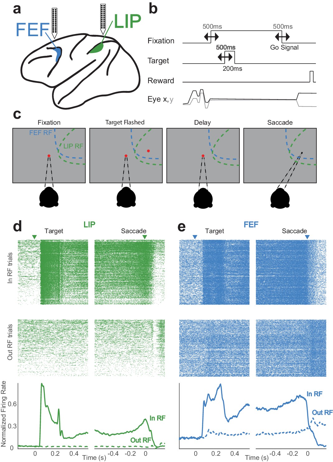
Memory-guided saccade task and simultaneously recorded neurons in LIP and FEF.
(a) Linear (stereotrode) probes (24–32 channels) were used to record in both LIP and FEF. (b) The timings of task events were varied continuously from trial to trial, making the delay (memory) period variable. (c) The monkey fixates and a target is flashed in the periphery (either ‘in’ or ‘out’ of the receptive fields); after a delay period (in which the monkey must maintain fixation) the fixation point is removed, indicating a ‘go-signal,’ and the monkey must make a saccade to where the target was. (d,e) Simultaneously recorded neurons in LIP (d) and FEF (e) with canonical responses. Each has a transient response to the visual target and a sustained response throughout the delay period (PSTH, bottom image). Even in these example neurons with strong persistent activity, there is significant variability during single trials (rasters, top image).
Figure 2 with 1 supplement

Population encoding model and analysis of example session.
(a) This generalized linear model (GLM)-based approach describes the time-varying spike rate of each neuron in terms of the external task events (i.e. the saccade target being flashed and the saccadic response), the recent spike-history of that neuron, and the activity of other simultaneously recorded neurons (within and across regions). The model is defined by three stages: 1) a linear stage that takes a weighted sum of the covariates and temporal filters, 2) an exponential point non-linearity that converts the linear output to a spike rate, and 3) conditionally Poisson spiking. (b–g) Each row corresponds to a neuron (1–3 in FEF, 4–8 LIP) and each column corresponds to the kernel of a particular predictor: (b) onset of the visual target; target in RF (solid line) and out RF (dashed line), (c) time of the saccade response, (d) recent spike-history and (e) coupling from other neurons (in LIP: green; in FEF: blue). Each kernel represents the time-varying gain on spiking for the fitted neuron due to the particular predictor while simultaneously accounting for the influence of the other predictors. (f,g) Each column displays the true PSTH (dashed lines) and predicted PSTH (solid lines) for each neuron (rows) for targets in (dark lines) and out (light lines) of the RF, aligned to the (f) target on and the (g) saccade. The predicted PSTHs were constructed from generating single-trial spike trains from the full population model for each neuron and averaging them.
Figure 2—figure supplement 1
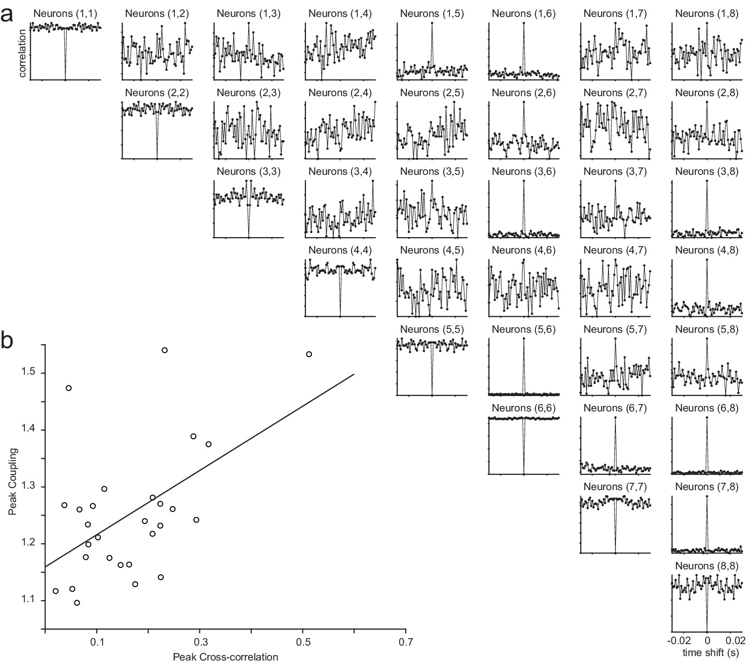
Cross-correlations of the example session (Figure 2) and the relationship between coupling and correlations.
(a) Cross-correlograms for all pairs of neurons in the example session. Center bin was removed from the autocorrelations for visualization purposes. (b) The relationship between peak coupling (estimated from the GLM) and the peak of the cross-correlations (R-squared = 0.57).
Figure 3 with 2 supplements
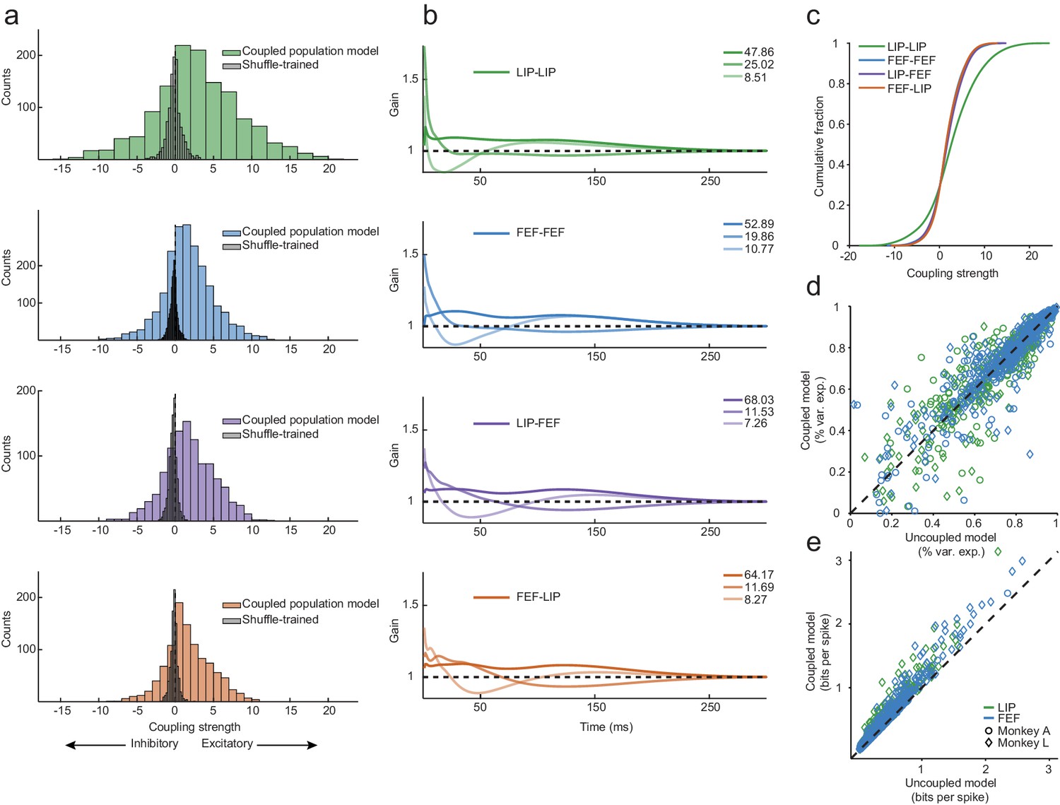
Exceptionally strong coupling both within and between areas.
(a) Distributions of raw coupling weights (colored histograms) defined by the sum of each kernel for each area interaction (LIP-LIP, FEF-FEF, LIP-FEF, FEF-LIP). Positive weights denote an excitatory interaction (the fitted neuron was more likely to spike given that another neuron just spiked) and negative weights indicate an inhibitory interaction (the fitted neuron was less likely to spike given that another neuron just spiked). A null distribution was constructed by shuffling the order of the trials for each neuron (gray histograms), effectively destroying the correlations between the ensemble of neurons but preserving the stimulus dependence and spike times. These distributions describe the probability of observing coupling due to chance alone (Wilcoxon rank-sum test, p=6.45×10−79; p=6.78×10−165; p=1.69×10−86; p=8.52×10−84). (b) Principal components analysis was performed on the coupling kernels split by each area interaction (as in (a)); the first three principal components (dark to light lines) accounted for around 90% of the variance (legend: variance explained for each PC). (c) Cumulative fraction of coupling weights for each interaction, corresponding to the distributions in (a). (d) Variance explained of the predicted PSTHs of the coupled model vs. the uncoupled model (median 76% variance explained under both models). Coupling was unnecessary to capture the average response of most neurons (the points fell near the unity line). (e) Predicted single-trial spike times (in units of bits-per-spike) of the coupled model vs. the uncoupled model. Coupling improved the predictions of the single-trial spike trains by 22% on average (25% for LIP; 19% for FEF; points fell above the unity line).
Figure 3—figure supplement 1
Absolute magnitudes of coupling and overall excitation and inhibition.
The core results held for a comparison of the absolute differences in coupling (a) as well as the overall (b) excitation and (c) inhibition (computed from the raw coupling weights across all kernels) for all area interactions.
Figure 3—figure supplement 2
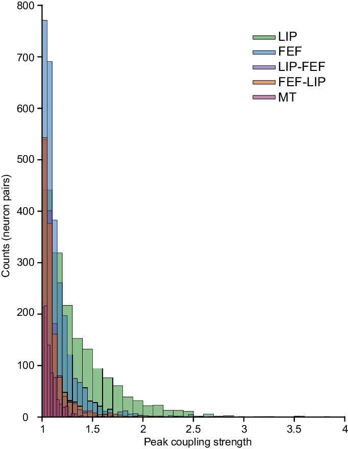
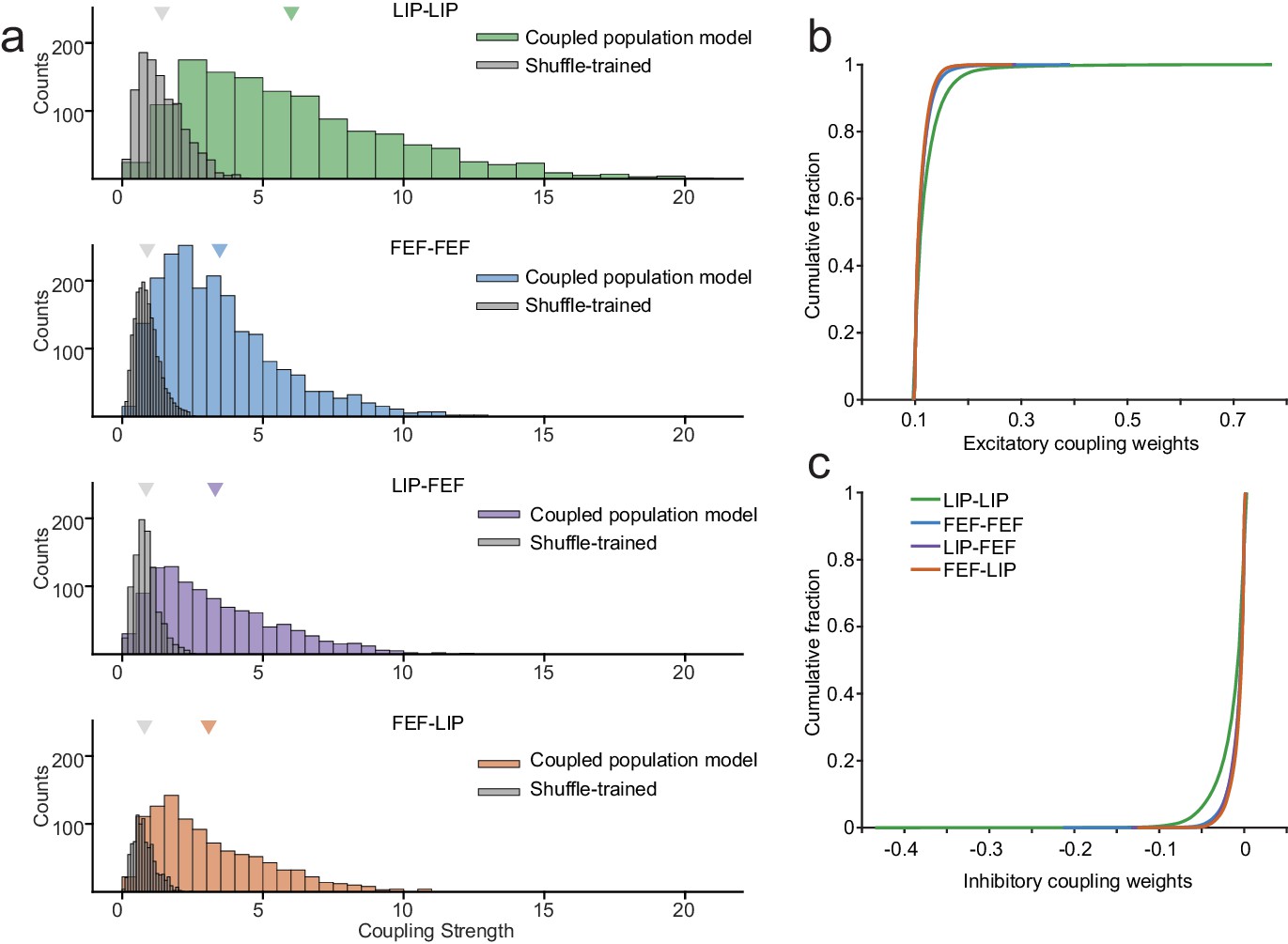
Distributions of max coupling kernels (gain).
Comparisons of MT with LIP-LIP, FEF-FEF, LIP-FEF, FEF-LIP, (Wilcoxon rank-sum test): p=2.19e-143; p=6.92e-103; p=2.18e-07; p=7.98e-22. Magnitude of the effect size (Cohen’s D): LIP-LIP = 0.89 (large effect), FEF-FEF = 0.41 (medium effect), LIP-FEF = 0.16 (small effect), FEF-LIP = 0.24 (small effect). MT data was collected during a perceptual decision making task under conditions reported previously (Yates et al., 2017).
Figure 4 with 1 supplement
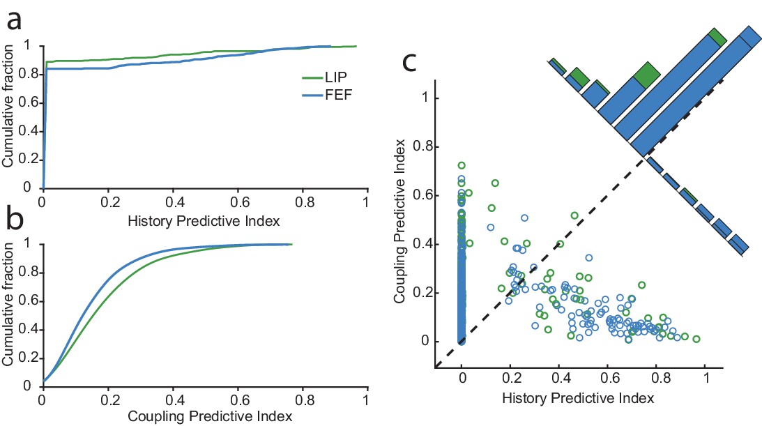
Network drive dominates circuit dynamics, especially in LIP.
For each neuron, we constructed predictive indices to further assess the influence of the spiking activity from other neurons (coupling) and itself (history). These indices are defined as the difference between the deviance explained by the model with or without history (a) or with or without coupling (b). (a) The cumulative fraction of history indices for neurons in each area. Overall, more neurons in FEF than LIP were impacted by their recent spike-history. (b) Same as in (a) but for coupling. Conversely, more neurons in LIP were influenced by the spiking activity of other neurons. (c) Comparison of the history and coupling indices. On the whole, spiking activity of neurons in both regions was more predicted by coupling than history (88.4% of neurons). For a large fraction of neurons, the history term was uninformative over and above the coupling and task terms (many neurons had a history index of zero). For a small subset of neurons (11%), predominantly in FEF, history had far more influence than coupling.
Figure 4—figure supplement 1

The relationship between persistent activity, coupling, and spike-history.
We compared the traditional measure of persistent activity (depicted by the size of circles in plot) quantified by calculating d-prime on the delay period activity (of the PSTH) between the target ‘in RF’ and ‘out RF’ conditions with measures of coupling and spike-history from the GLM. There was little relationship between the classic trial-average measure of persistent activity and estimates of coupling and spike-history effects on single trials (‘PA’=persistent activity; Pearson’s r, LIP: coupling/PA: R = −0.07; history/PA: R = −0.08; FEF: coupling/PA: R = −0.12; history/PA: R = −0.007).
Figure 5
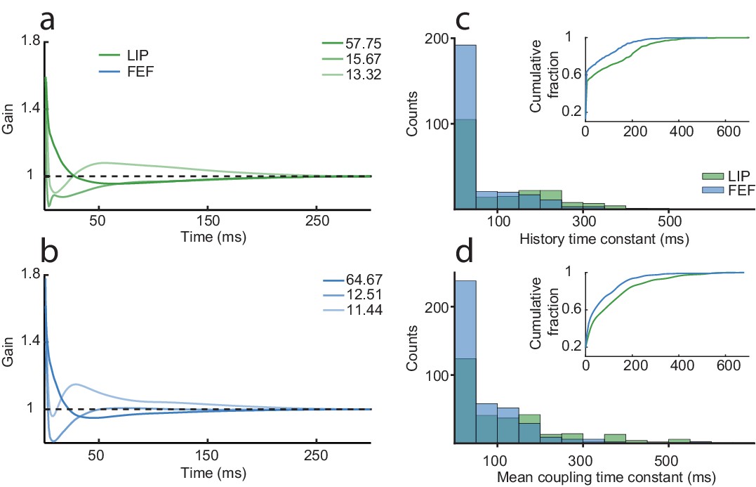
Spike-history and coupling time constants are similar but longer in LIP than FEF.
The first three principal components for the history kernels in LIP (a) and FEF (b), which capture the spike-history time constant of the neurons, while controlling for the task and coupling drive. The dominant component in both areas was a slow decay. An exponential curve was fit to the history kernel of each neuron to estimate a time constant (tau). (c) The distribution of spike-history time constants differed between areas (Wilcoxon rank-sum test, p=1.20×10−06; LIP mean = 99.6 ms; FEF mean = 68.2 ms). Most neurons had short time constants, but there was a ‘long tail’ of neurons with much longer time constants (100–300 ms). (d) Same as (c) but for the mean coupling kernel of each neuron. Coupling time constants were larger overall than history time constants and also differed between areas (Wilcoxon rank-sum test, p=6.43×10−07; LIP mean = 133.8 ms; FEF mean = 76.5 ms). Insets shows the cumulative distributions of the time constants; LIP had more neurons than FEF with long coupling and history time constants.
Figure 6 with 2 supplements
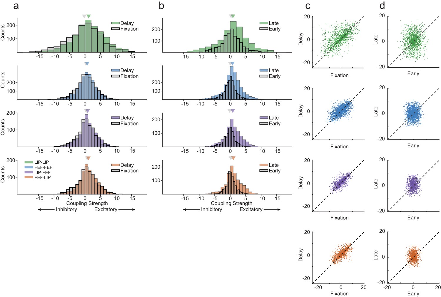
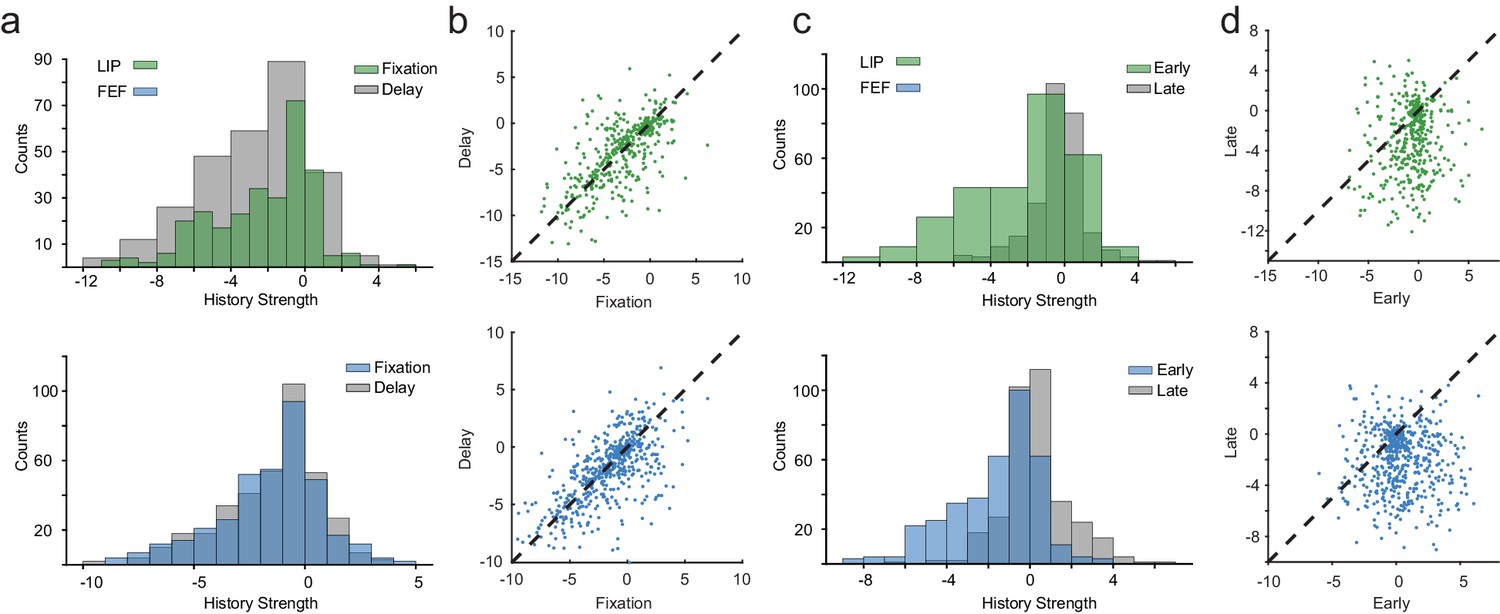
Interneuronal coupling is dynamic across behavioral epochs.
(a) The strength of coupling increased between the fixation period and delay period across all area interactions, especially within LIP (Wilcoxon rank-sum test, p=4.87×10−09; p=5.17×10−04; p=1.64×10−04; p=3.01×10−03). Strong coupling was observed even during fixation. (b) Coupling increased from early in the delay period to late in the delay across all area interactions (Wilcoxon rank-sum test, p=1.08×10−06; p=1.65×10⁻²⁷; p=3.96×10⁻²³; p=1.97×10⁻¹⁷). LIP exhibited increases in excitatory and inhibitory interneuronal interactions, whereas FEF and between area interactions were dominated by increases in excitatory connectivity. (c) Interneuronal coupling between the fixation and the delay period was systematic (Pearson’s r, R = 0.61; R = 0.66; R = 0.70; R = 0.72), (d) whereas the coupling strength between early and late in the delay showed no relationship (Pearson’s r, R = 0.04; R = 0.04; R = 0.06; R = 0.03).
Figure 6—figure supplement 1
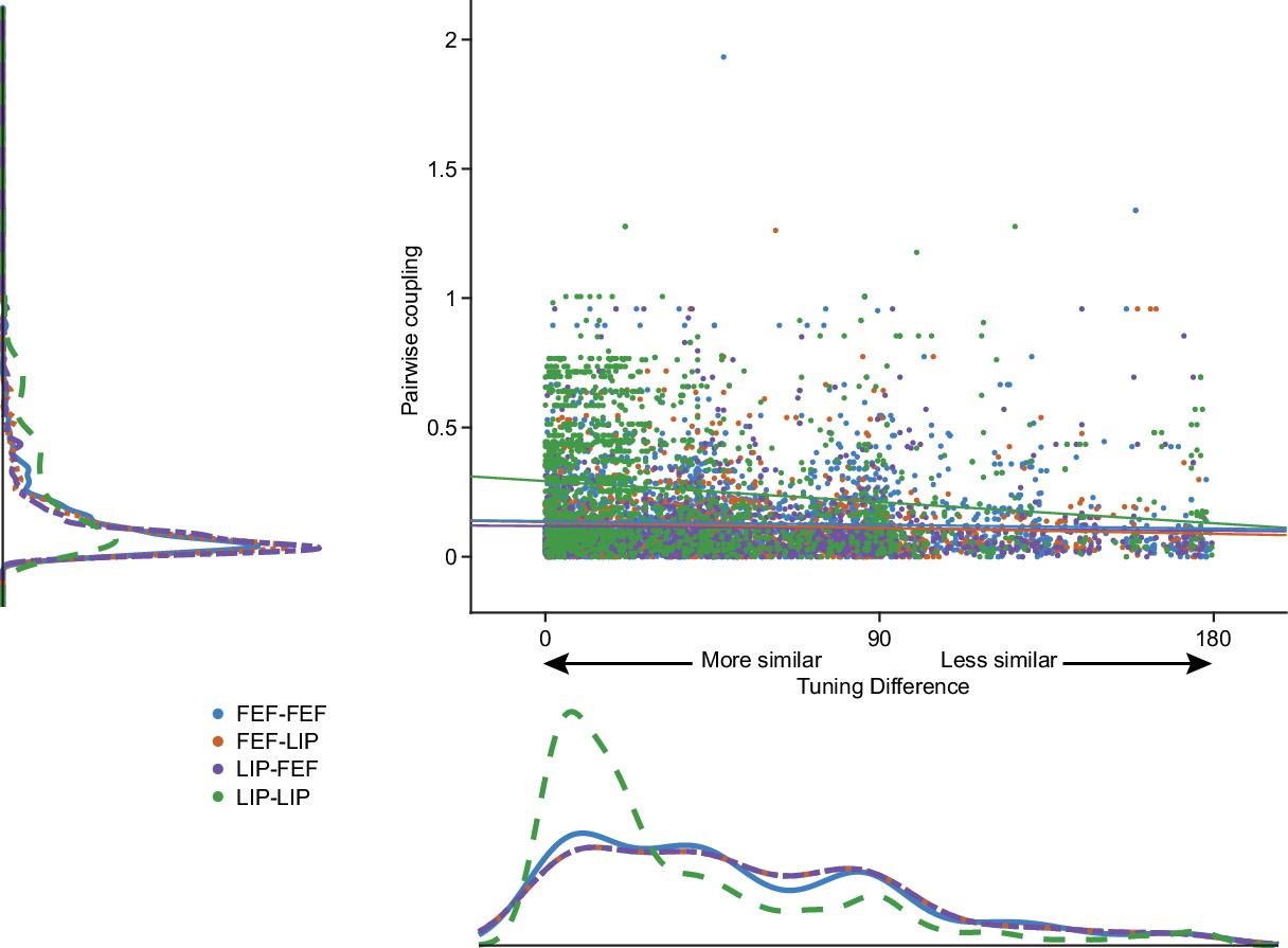
Pairwise coupling as a function of spatial tuning similarity.
Classic models of persistent activity suppose that neurons with similar tuning properties should be more coupled. The absolute max of the coupling kernel weight for each neuron pair is plotted as a function of tuning similarity. The difference in selectivity was calculated by fitting a 1D circular Gaussian tuning curve to the responses of each neuron at each target location and taking the difference between the peak of the tuning curves for each pair of neurons (smaller numbers means more similar). Lines are least-squares fit (R-squared: LIP-LIP: −0.16, FEF-FEF: −0.05, LIP-FEF: −0.03, FEF-LIP: −0.08).
Figure 6—figure supplement 2
Spike-history dynamics over behavioral epochs.
(a) Distributions of max spike-history weights in LIP and FEF for the fixation and delay periods. History dynamics were consistent across the fixation and delay. (b) The pairwise relationship between spike-history between fixation and delay for LIP and FEF (Pearson’s r, R = 0.67; R = 0.64). (c) Distributions of max spike-history weights in LIP and FEF for early and late in the delay period. (d) The pairwise relationship between spike-history between early and late in the delay for LIP and FEF (Pearson’s r, R = 0.13; R = −0.03). Spike-history weights shifted from negative to positive from early to late in the delay, predominately in FEF.
Figure 7 with 2 supplements
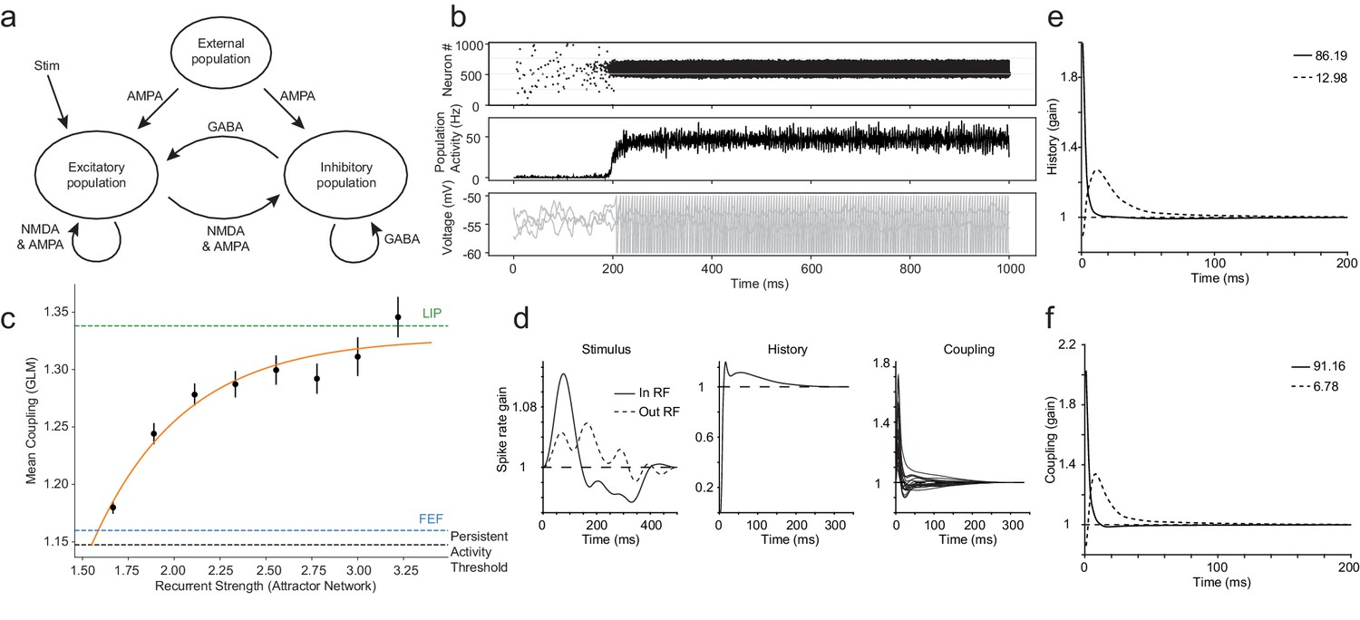
Coupling differences in LIP and FEF can be explained by the strength of recurrent connectivity in attractor networks.
Synthetic datasets were generated from a classic attractor network and fit with the GLM using the same procedure used with the real data. (a) Schematic of classic attractor network used to model spatial working memory (adapted from Gerstner et al., 2014). (b) Population activity of attractor network for an example session with high recurrent strength (2.3): a stimulus triggers selective persistent activity (top, middle row); voltage traces from three example neurons (bottom row). (c) A systematic relationship was revealed between the mean coupling (estimated from the fitted GLM) and the internal recurrent strength of the attractor network (error bars = SEM). The black dashed line indicates the level of coupling at the minimum recurrent strength necessary to generate persistent activity. The green and blue lines are LIP and FEF’s coupling determined from the data, respectively. (d) Stimulus, spike-history, and coupling kernels of an example neuron. PCA of history (e) and coupling (f) kernels for an example session revealed the ‘fast’ and ‘slow’ dynamics of the neurons specified in the network, which accounted for virtually all the variance explained (legend).
Figure 7—figure supplement 1
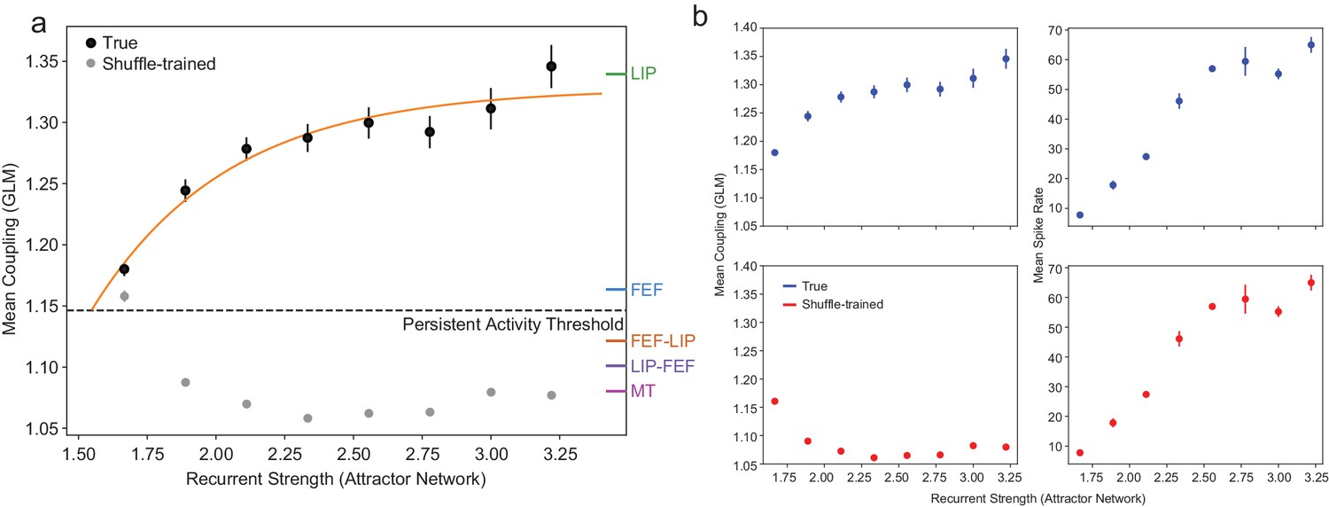
The relationship between coupling (GLM) and recurrent strength (attractor network) for the other area interactions and the shuffling control.
(a) As in Figure 7, including coupling values for LIP-FEF, FEF-LIP, and MT. Gray points are coupling values from the GLM trained on permuted data (as explained in the methods; error bars are so small as to be invisible for most points). As expected, disrupting the correlational structure of the population eliminates the relationship between coupling and the recurrent strength. The small increase in coupling at the lowest recurrent strength in the shuffled condition is artificially inflated due to the very few spike trains that are sampled from the network at this parameter value (the network is producing very little activity and is only borderline persistent), and the identical nature of the artificial neurons. (b) Controlling for overall firing rate differences between ROIs with shuffling. Coupling and mean firing rates increase with recurrent strength under normal conditions (top row). During the shuffling control (bottom row), the coupling is reduced to chance levels but the mean firing rates are identical, showing that coupling tracks the internal recurrent strength of the attractor network and not simply overall increases in firing rate (error bars so small as to be invisible at most points). This is bolstered by the fact that neurons in FEF actually had a significantly higher mean firing rate than LIP, whereas LIP had much stronger coupling than FEF (see Materials and methods).
Figure 7—figure supplement 2
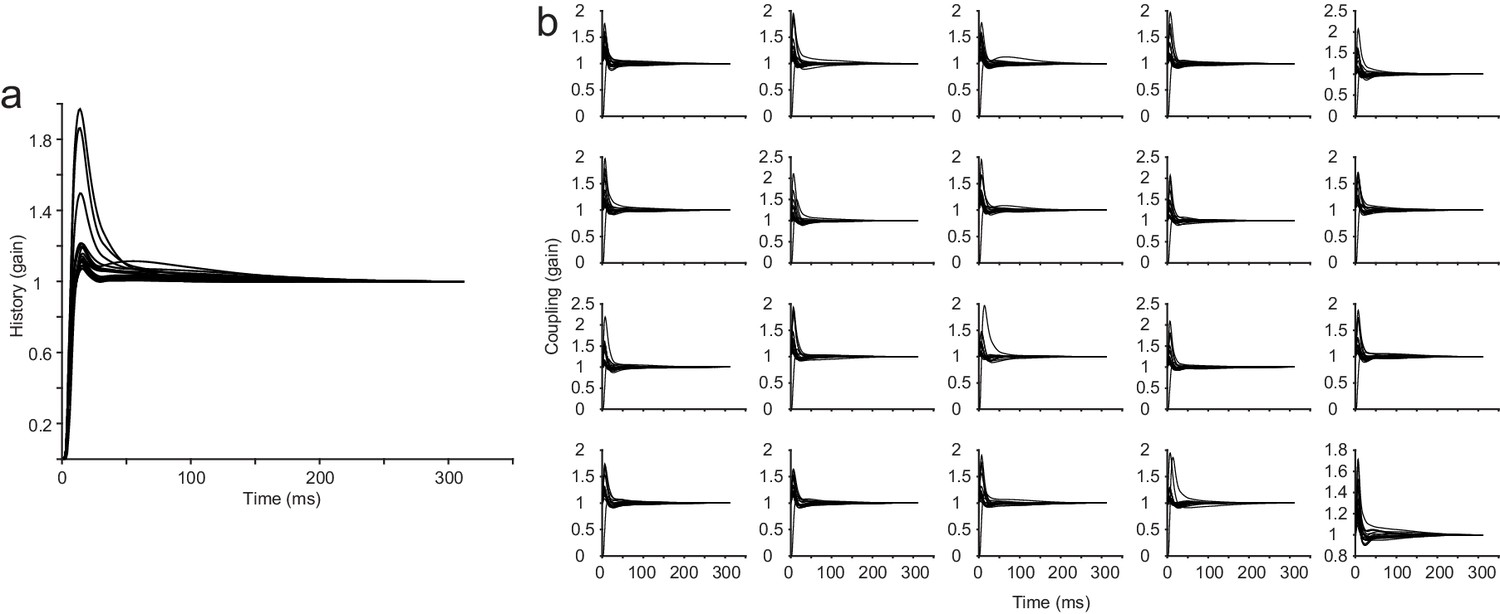
All history and coupling kernels from an example session from the attractor network.
The parameter for the recurrent strength of the attractor network was 2.3 (a network that can generate strong persistent activity). (a) History kernels from the GLM for all neurons in the example session (N = 20). (b) Coupling kernels from the GLM for all neurons in the example session, each neuron has N-1 coupling kernels in the fully coupled model.
Additional files
Download links
A two-part list of links to download the article, or parts of the article, in various formats.
Downloads (link to download the article as PDF)
Open citations (links to open the citations from this article in various online reference manager services)
Cite this article (links to download the citations from this article in formats compatible with various reference manager tools)
Recurrent circuit dynamics underlie persistent activity in the macaque frontoparietal network
eLife 9:e52460.
https://doi.org/10.7554/eLife.52460


