Navigating the garden of forking paths for data exclusions in fear conditioning research
- University Medical Center Hamburg Eppendorf, Germany
- University of Würzburg, Germany
- Erasmus University Rotterdam, Netherlands
- KU Leuven, Belgium
- University of Amsterdam, Netherlands
- Ruhr University Bochum, Germany
- Utrecht University, Netherlands
- University of Greifswald, Germany
- University of Potsdam, Germany
Figures
Figure 1
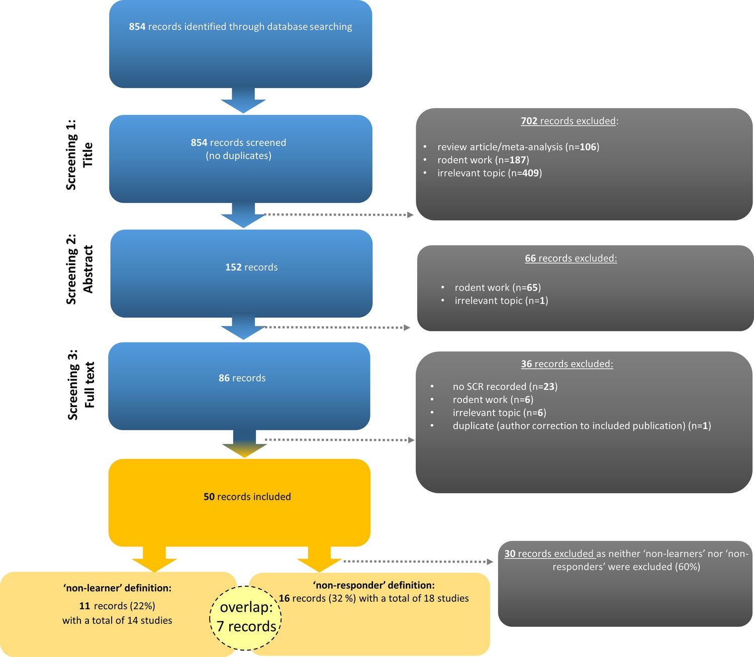
Flow chart illustrating the selection of records according to PRISMA guidelines (Moher et al., 2009).
Note that seven records (14%) employed the definition and exclusion of both ‘non-learners’ and ‘non-responders’. Examples of irrelevant topics included studies that did not use fear conditioning paradigms (see https://osf.io/uxdhk/ for a documentation of excluded publications).
Figure 2
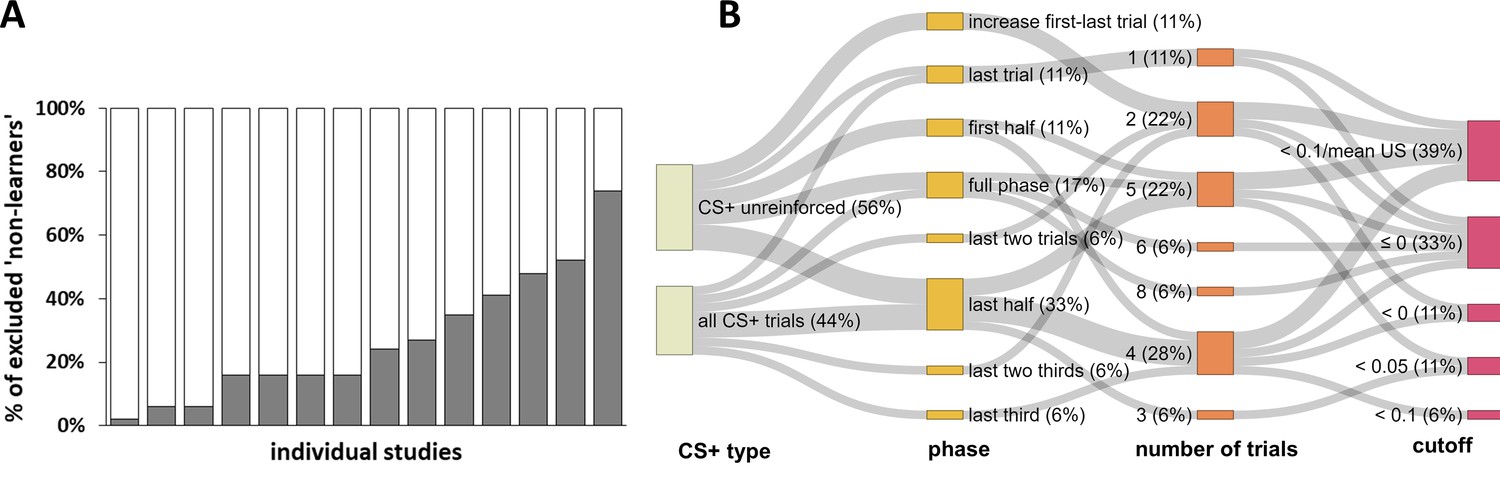
Graphical illustration of the percentage of ‘non-learners’ and forking path analysis across studies.
(A) Illustration of the percentage of participants excluded (‘non-learners’) based on SCR CS+/CS–discrimination scores across studies included in the systematic literature search (note that these 14 individual studies are derived from 11 different records, as three records reported two individual studies each). Please note that some studies excluded participants on the basis of ‘non-learning’ as well as ‘non-responding’ (cf. Figure 1), and hence the percentages displayed here do not necessarily map onto the percentage of total participants excluded per study. Also note that the study with the highest percentage of excluded participants (i.e., 74%) reported the percentage of excluded participants as a single value that included ‘non-learners’ and ‘non-responders’. This study is only included here because the largest proportion of exclusions can be expected to result from ‘non-learning’. (B) Sanky plot showing the ‘forking paths’ of performance-based exclusion of participants as 'non-learners', illustrating differences in the experimental phase, number of trials, the SCR CS+/CS– discrimination score in µS used to define a ‘non-learner’, the CS+ type considered (illustrated as the nodes in graded colors) and their combinations used to define 'non-learners' across studies. Path width was scaled in relation to frequency of the combinations. Note that for some ‘nodes’ the percentages do not add up to 100% because of rounding.
Figure 3 with 1 supplement
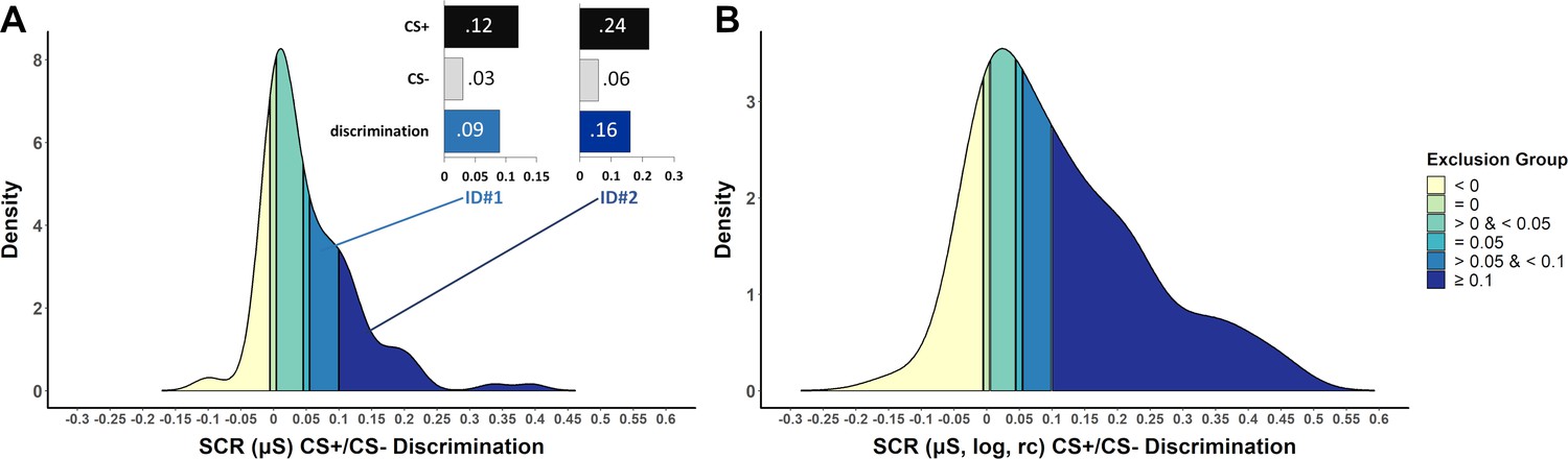
Density plots illustrating the frequency of CS+/CS– discrimination scores in a sample of N = 116 (Data set 1) based on the last half of the acquisition phase (including 7 CS+ and 7CS–, 100% reinforcement rate) for (A) SCR raw data and (B) logarithmized and range-corrected (rc; individual trial SCR/SCRmax_across_all_trials) SCR data (as it is typically not reported to which data exclusion criteria are applied).
Color coding (yellow to blue) illustrates which part of the sample would be excluded when applying the performance-based exclusion criteria (i.e. CS+/CS– discrimination) as identified by the systematic literature search. Panel (A) also illustrates two case examples (ID#1 and ID#2) that differ in SCR amplitudes but importantly show the same discrimination ratio between CS+ and CS– (4:1). These two case examples illustrate that high CS+/CS– discrimination cutoffs favor individuals with high SCR amplitudes to remain in the final sub-sample. Data are based on a re-analysis of an unpublished data set recorded in the fMRI environment (Klingelhöfer-Jens M., Kuhn, M. and Lonsdorf, T.B.; unpublished).
Figure 3—figure supplement 1
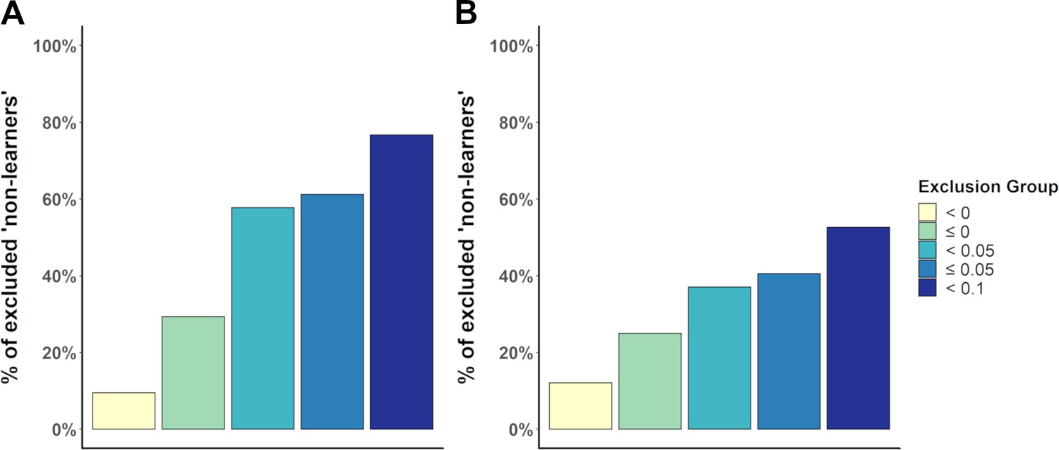
Percentages of participants excluded (Data set 1) when employing the different CS+/CS– discrimination cutoffs (as identified by the systematic literature search and graphically shown in Figure 3B) which are illustrated as density plots in Figure 3.
Percentages are calculated on the basis of (A) raw SCR scores or (B) logarithmized and range-corrected scores in Data set 1. Note that the different groups are cumulative (i.e., the darker colored groups also comprise the lighter colored groups).
Figure 4 with 1 supplement
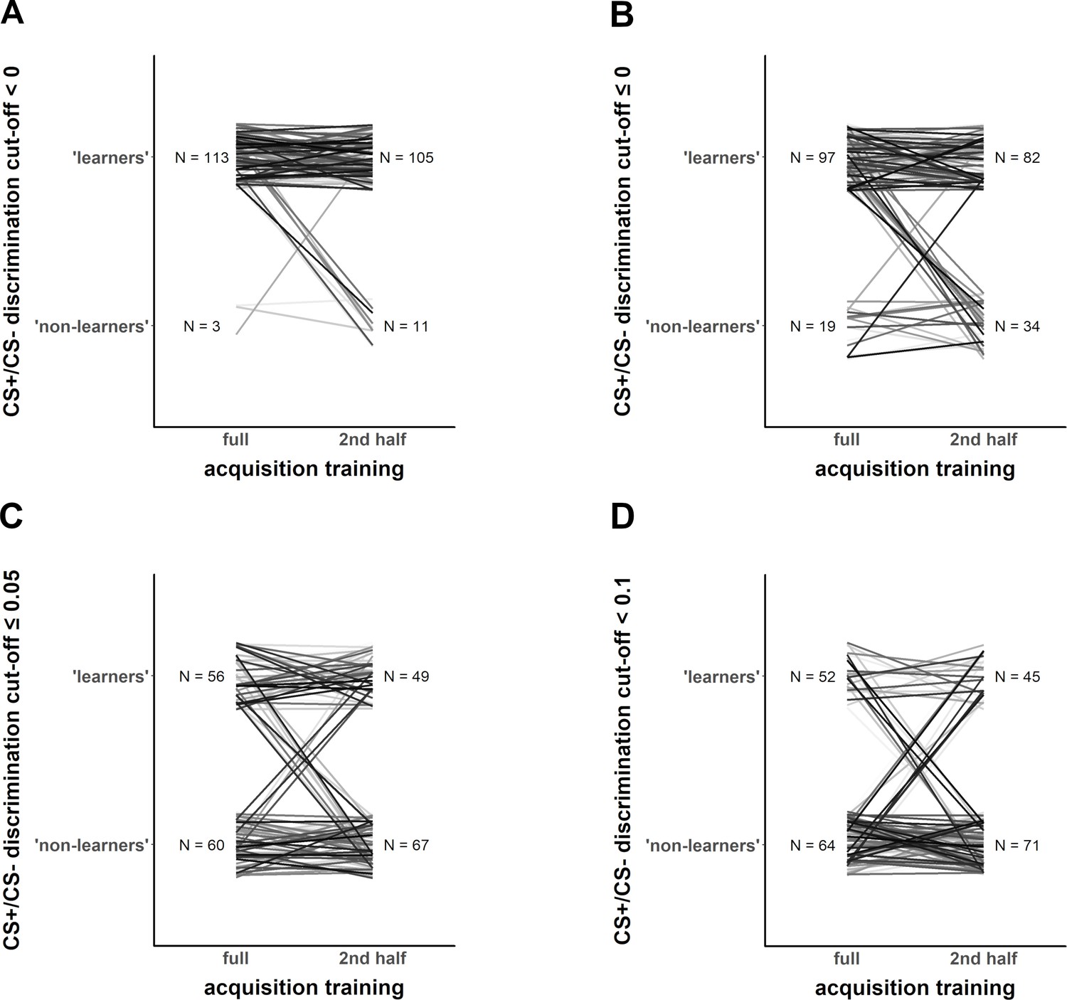
Exemplary illustration of individuals (Data set 1) that switch from being classified as ‘learners’ vs. ‘non-learners’ depending on the different CS+/CS– discrimination cutoff level (panels A–D), when calculation of CS+/CS– discrimination is based on either the full fear acquisition phase or the second half of the fear acquisition training (left and right part of each panel, respectively).
Figure 4—figure supplement 1
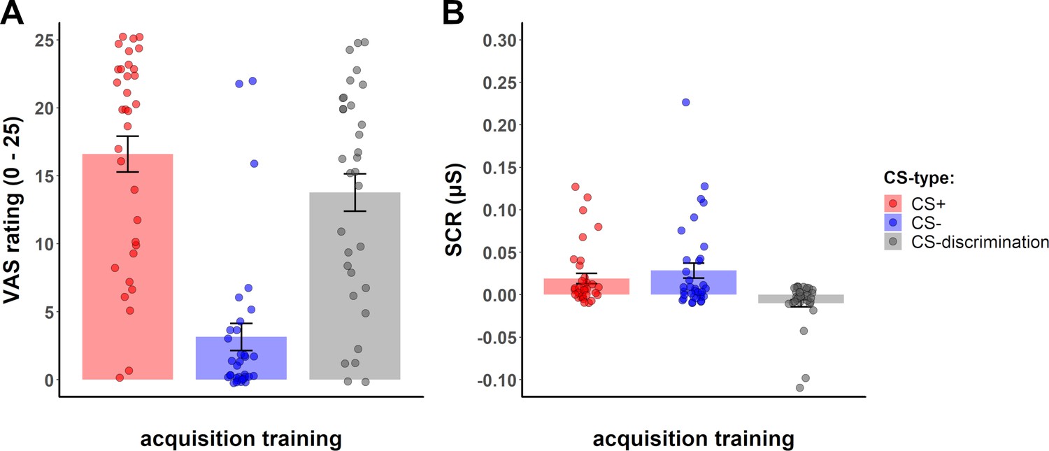
Bar plots (mean ± SE) on which the superimposed individual data points show CS+ and CS– amplitudes (of raw SCR values) and CS+/CS– discrimination in (A) fear ratings and (B) SCRs raw values in the group of ‘non-learners’, as exemplarily defined for this example as a group consisting of individuals in the two lowest SCR CS+/CS– discrimination cutoff groups (i.e., ≤0) in Data set 1.
This illustrates that individuals who fail to show CS+/CS– discrimination in SCRs (B) may in fact show substantial CS+/CS– discrimination (as an indicator for successful learning) in other outcome measures, as exemplarily illustrated here for fear ratings (A).
Figure 5
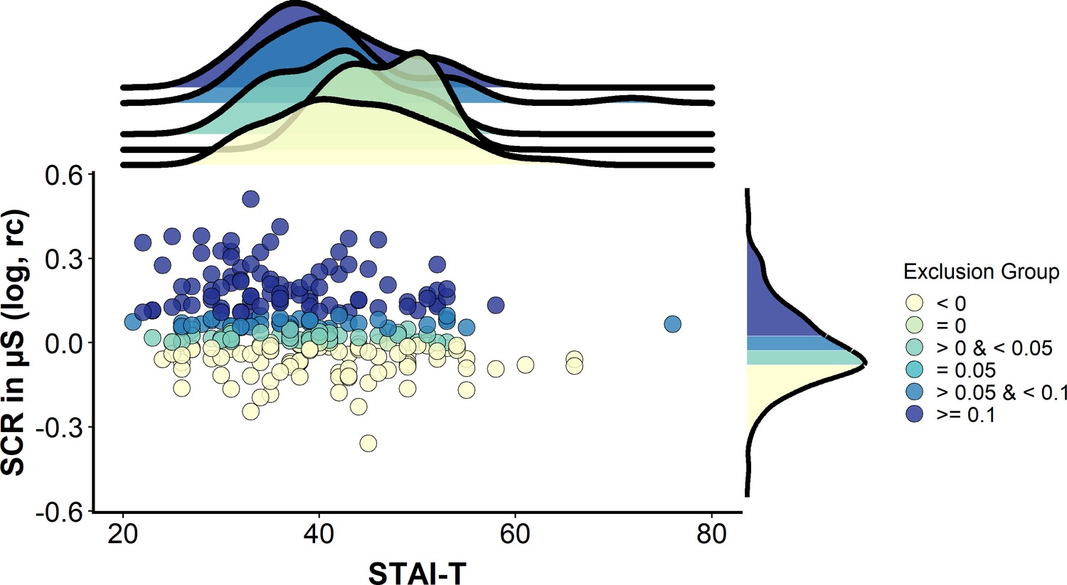
A case example illustrating potential sample bias induced by excluding individuals on the basis of CS+/CS– discrimination scores (based on logarithmized, range-corrected (rc) SCR data).
Scatterplot illustrating the association between trait anxiety (measured via the trait version of the State-Trait Anxiety Inventory, STAI-T) and CS+/CS– discrimination scores in a sample of N = 268 (Data set 2). Color coding (yellow to blue) illustrates which part of the sample would be excluded when applying the performance-based exclusion criteria (i.e. CS+/CS– discrimination) as identified by the systematic literature search. Note that within this sample, no individuals were identified with CS+/CS– discrimination equaling 0.05 µS. The upper panel illustrates densities for trait anxiety for the different CS+/CS–discrimination groups. The rightmost panel illustrates the density for CS+/CS– discrimination in the full sample. Data are based on a re-analysis of a data set recorded in the behavioral environment (Schiller et al., 2010). Note that despite the different color coding, which serves illustrative purposes only, the groups are in practice cumulative. More precisely, the groups illustrated by lighter colors are always contained in the darker colored groups when applying the respective cutoffs. For example, the group excluded when employing a cutoff of <0.1 µS (mid blue) also comprises the groups already excluded for the lower cutoffs of = 0.05 µS (light blue), <0.05 µS (turquoise), = 0 µS (light green) and <0 µS (yellow). For illustrative purposes, the different groups are treated as separate groups in this figure.
Figure 6
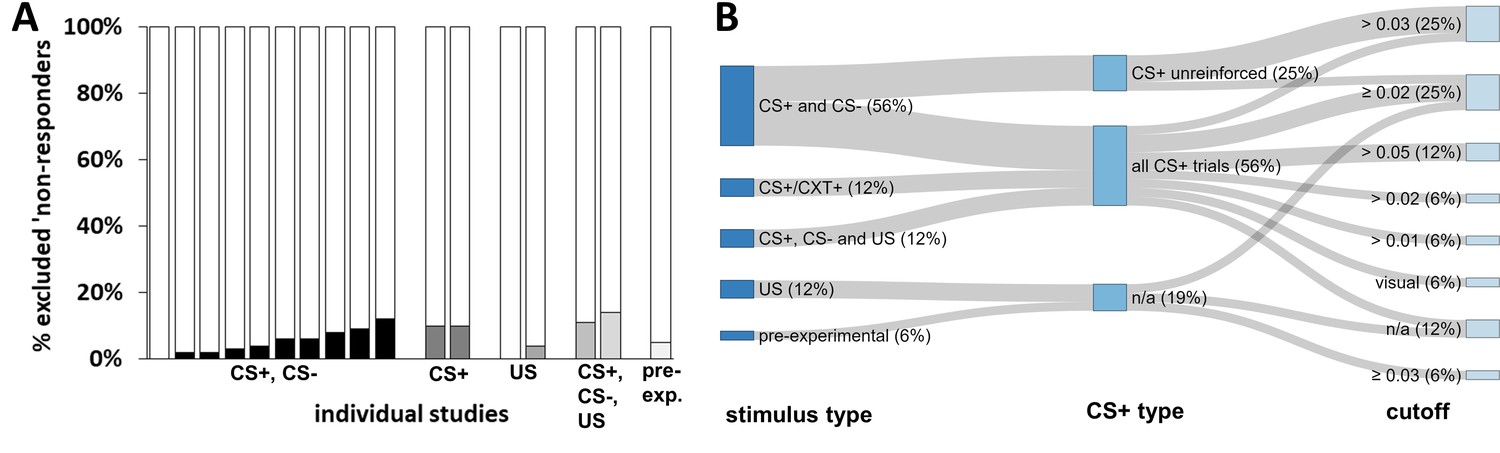
Graphical illustration of the percentage of ‘non-responders’ and forking path analysis across studies.
(A) Illustration of the percentage of participants excluded from each study as a result of ‘ SCR non-responding’ to (i) the conditioned stimuli (i.e., CS+ and CS–), (ii) the US, (iii) the CS+ (which also comprises a study that used the CXT+, i.e. context), (iv) the CS+, CS– and US or (v) a pre-experimental test. Note that these 18 individual studies are derived from 16 different records, two of which included two different studies that used the same criteria. Note that some studies excluded participants on the basis of ‘non-learning’ as well as ‘non-responding’, and hence the percentages displayed here do not necessarily map onto the percentage of total participants excluded from each study. Also note that a single study (Schiller et al., 2018) is not included in this visualization because it reported % ‘non-learners’ and % ‘non-responders’ as a single value. This value has been included in the visualization of ‘non-learners’ (Figure 2) as these are expected to represent the largest proportion. (B) Sanky plot illustrating the stimulus type (pre-experiment refers to determination of 'responding' in an unrelated phase prior to the experiment), the minimally required response amplitude in µS (note that ‘visual’ refers to visual inspection of the data without a clear-cut amplitude cutoff, NA refers to no criterion applied) illustrated as the nodes in graded colors and their combinations that lead to classification as a ‘non-responder’. Path width was scaled in relation to frequency of the combinations. Note that for some ‘nodes’ the percentages do not add up to 100% because of rounding.
Figure 7
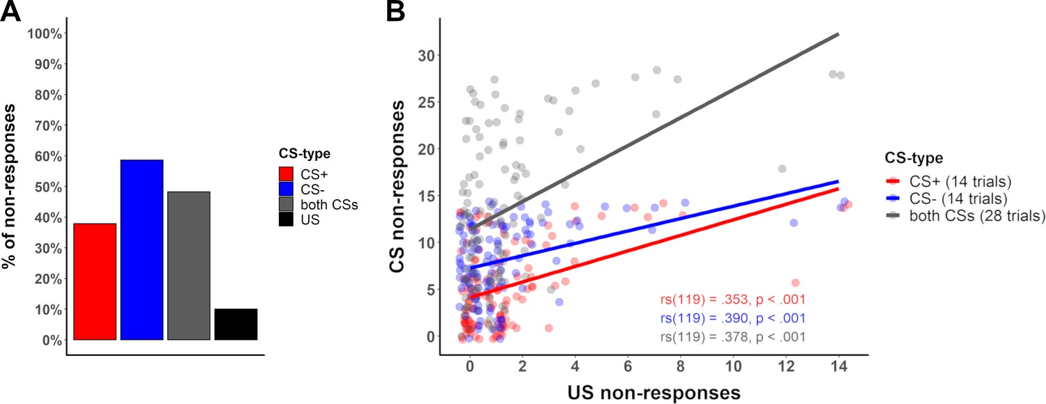
Percentage of no-responses across stimuli and correlation between CS and US non-responses.
(A) Bar plot displaying the number of ‘non-responses’ to the CS+, CS–, across both CS and to the US across all participants in Data set 1 (see Appendix 4—table 1 for percentages across different data sets). (B) Scatterplot illustrating the number of ‘non-responses’ (i.e., zero-responses, here defined by an amplitude <0.01 µS) to the US presentations (total of 14 presentations) and the CS+ (red) and CS– (blue) responses (14 presentations each) for each participant in Data set 1. For completeness sake, ‘non-responses’ across CS types are illustrated in gray (CS+ and CS– combined, total of 28 presentations). Lines illustrate the Spearman correlation (rs) between ‘non-responses’ to the US and ‘non-responses’ to the CS+, CS– and both CS, with corresponding correlation coefficients (font color corresponds to CS type) included in the figure.
Tables
Appendix 1—table 1
Summary of criteria used to define ‘non-learners’ across records included in the systematic literature search.
Criteria used to define ‘non-learners’ were identified in eleven records reported in a total of 14 individual studies.
| Reference | % excluded participants (‘non-learners’) | CS+/CS– cut-off (in µS) for ‘non-learners’ | N trialsacq total CS+/CS– | N trialsacq considered CS+/CS– | Trials phase (unless otherwise stated, this refers to fear acquisition training) | Additional criteria/notes |
|---|---|---|---|---|---|---|
| Ahmed and Lovibond, 2019, Exp. 1 | 24% | <or = 0 | 3/3 | 2/2 | last two thirds | only considered as ‘non-learners’ if applicable to both SCL and ratings |
| Ahmed and Lovibond, 2019, Exp. 2 | 16% | |||||
| Reddan et al., 2018a | 35% | <or = 0 | 16/8 | 8b/8 | full phase | |
| Grégoire and Greening, 2019 | 16% | <0.1 | 13c/8 | 4c/4 | last third | participants were also excluded if they did not show equivalent responding to both CS+s (difference > 0.1 µS) or when not showing equal extinction to both CS+s or complete differential extinction to both CS+s vs. CS– (difference > 0.1 µS) |
| Hu et al., 2018 | 6% | <or = 0 | 16/10 | 5/5d OR 1/1 | second halfd OR last triald | ‘non-learners’ discontinued after day 1 of the experiment |
| Oyarzún et al., 2019, Exp. 1 | 27% | <or = 0e | eightc/8 | 4c/4 | second half | only considered as ‘non-learners’ if applicable to both SCR and fear-potentiated startle |
| Oyarzún et al., 2019, Exp. 2 | 41% | |||||
| Belleau et al., 2018 | 2% | <0.05 | 5/5 | 5/5 | full phase | only considered as ‘non-learners’ when also failing to show any differential ratings (i.e.,<or = 0 in discrimination)f |
| Morriss et al., 2018 | 6% g | < or = 0h | 12/6 | 6b/6 | full phase | only considered as ‘non-learners’ if applicable across all phases (fear acquisition and extinction training, avoidance acquisition and extinction) |
| Schiller et al., 2018; Schiller et al., 2010, Exp. 1 | 48%i | <0.1/mean SCR to the US | 16c/10 13c/8 | 5b /5 OR 5b /5 OR 1b /1 OR increase from first to last trial 4b /4 OR 4b /4 OR 1b /1 OR increase from first to last trial | first half of acquisition OR second half OR last trial of acquisition, OR the increase from the first to last trial of acquisition | |
| Schiller et al., 2018; Schiller et al., 2010, Exp. 2 | 74%i | |||||
| Nitta et al., 2018 | 52% | <0 | 13c/8 | 2c /2 | last two trials | one additional participant showed strong SCR during re-extinction phase to CS+ and was therefore excluded |
| Hartley et al., 2019 | 16% | <or = 0.05 | 6/6 | 3/3 | last half | |
| Hu et al., 2019 | 16% | < 0k | 8b/8 | 4b/4 | second half |
-
aPersonal communication with D. Schiller (20.5.2019 and 30.8.2019) confirmed that individuals were classified as ‘non-learners’ when they ‘did not demonstrate greater SCRs to the CS+ relative to the CS– on average across all acquisition trials (n = 24)’ (see 'Materials and methods' section). The personal communication clarified that the statement included in the results section that defines ‘non-learners’ as individuals that “did not demonstrate a discriminatory SCR during acquisition, defined as greater SCR to the CS+ relative to the CS– during either the first or last half of threat-acquisition on average’ was intended to refer to the same procedure (i.e., the full acquisition phase).
bRefers to unreinforced CS+ trials (CS+ trials not followed by the US) only.
-
cFor each CS+1 and CS+2.
dPersonal communication with D. Schiller (1.5.2019): late acquisition as reported in the publication refers to the last half or last trial. Anyone that had a positive difference (>0.000 µS) in either the second half or last trial of acquisition was kept.
-
ePersonal communication with J. Oyarzun (21.5.2019): all difference scores > 0 µS were considered as CS+/CS– discrimination.
fPersonal communication with E. Balleau, PhD (5.5.2019): ‘differential ratings’ means that CS+>CS is equal to or below 0 µS was non-differentiation.
-
gThese were not excluded as results did not change.
hPersonal communication with J. Morriss (15.4.2019): no positive differential response is defined as any number <0 µS.
-
iPercentages for ‘non-learners’, ‘non-extinguishers’ and ‘non-responders’ reported together.
kPersonal communication with D. Schiller (21.5.2019): zero differences were kept.
Appendix 1—table 2
Summary of criteria used to define ‘non-responders’ across records included in the systematic literature search.
Fifteen records, reporting a total of 17 studies, were identified.
| Record | % excluded participants (‘non-responders’) | Cut-off (in µS) for a valid SCR | Valid responses in at least % of trials | Stimulus type (also referred to as ‘trial’) on which the exclusion is based | Additional criteria/notes |
|---|---|---|---|---|---|
| Baeuchl et al., 2019 | 10% | >0.01 | ≥66% | CXT+ | |
| Tuominen et al., 2019 | 12% | >0.05 | ≥13% | CS+ and CS– | |
| Gruss and Keil, 2019 | 11% | visual inspectiona | CS+, CS–and US | ||
| Sjouwerman and Lonsdorf, 2019 | 14% | ≥0.02 | US:≥67% CS: no valid response in each CS modality | CS+, CS– and US | |
| Grégoire and Greening, 2019 | 8% | >0.02 | ≥25%b | CS+ and CS–c | |
| Hu et al., 2018 | 3% | ≥0.02 | 100% | CS+ and CS–c | ‘non-responders’ discontinued after day 1 of the experiment |
| Oyarzún et al., 2019, Exp. 1 | 0% | ≥0.02 | ≥25% | CS+d and CS–c | |
| Oyarzún et al., 2019, Exp. 2 | 9% | ||||
| Tani et al., 2019 | 10% | >0.03e | 100% | CS+ | |
| Marin et al., 2019 | 0%f | ≥0.03 | ≥10% | US | |
| Taylor et al., 2018 | 5% | NA | 100% | motor testg | |
| Morriss et al., 2018 | 6% | >0.03 | ≥90% | CS+d and CS–c | only applicable if true across all phases/days of the experiment |
| Schiller et al., 2018; Schiller et al., 2010, Exp. 1 | 48%h | ≥0.02 | ≥25% | CS+d and CS– | |
| Schiller et al., 2018; Schiller et al., 2010, Exp 2 | 74%h | ||||
| Morriss and van Reekum, 2019, Exp. 1 | 2% | >0.03 | >90% | CS+d and CS– | |
| Morriss and van Reekum, 2019, Exp. 2 | 2% | ||||
| Hartley et al., 2019 | 6% | <0.05i | ≥33 %i | CS+ and CS–c | |
| Hu et al., 2019 | 4% k | ≥0.02 | 100% k | US | |
| Leuchs et al., 2019 | 4% | NA | ≥33% | CS+ and CS–c | only applicable if true across both days of the experiment |
-
aPersonal communication with L. Forest Gruss (29.4.2019): “the determination of non-responders was done, this was done on visual inspection by me through all trials of all individuals. I verified after determining who the lowest, i.e. non-responders were, in the same fashion as the startle non-responders in summing responding over the entire experiment, and this responding falling below a threshold of overall response (~<10%) AND one individual due to lack of response at the end of the trial to the UCS specifically".
bPersonal communication with S.G. Greening (24.4.2019): “non-responders if more than 75% of data were missing (i.e., SCR <0.02 μS) during the training phase. So, that means, if a participant had at least six trials (out of 24) with measurable SCRs (whatever the condition), we kept them (if the other acquisition criteria were OK, see below). If they had five trials or fewer with measurable GSR, we considered them a non-responder and removed them".
-
cPersonal communications that ‘trial’ or this statement refers to CS+ and CS– trials: S. Greening (24.4.2019), D. Schiller (1.5.2019), J. Oyarzun (21.5.2019), J. Morriss (15.4.2019), C. Hartley (2.5.2019), V. Spoormaker (18.4.2019).
d CS+ unpaired.
-
ePersonal communication with H. Tani (2.5.2019): only CS+ trials were considered (here as response to the sound or the intrapersonal stimulus).
fPersonal communication with M.-F. Marin (23.4.2019): exclusion criteria were defined, but no participant met these criteria and hence none was excluded.
-
gPersonal communication with V. Taylor (6.6.2019): clarified that "non-responders’ were identified in a “motor test of SCR responding during the preliminary session. Essentially, they had to compress a ball with the right hand with maximal physical force for a few seconds on about 10 trials, which typically elicits quite large SCRs in subjects. Failure to respond to an SCR to all of these trials was considered a non-responder".
hPercentages for ‘non-learners’, ‘non-extinguishers’ and ‘non-responders’ reported together.
-
iPersonal communication with C. Hartley (2.5.2019): clarified that “participants were considered non-responder if they had SCR values of 0 for more than 8 of the 12 trials in acquisition (<4 responsive trials)”.
k The percentage of ‘non-responders’ and ‘non-learners’ was reported together without percentages for each category; personal communication with D. Schiller (21.5.2019): in the paper, it is reported that five individuals ‘were excluded due to equipment malfunction (N = 2) or had non-measurable skin conductance response (SCR) to the shock (N = 3)”. It was confirmed that these individuals excluded for non-measurable SCR did not show any responses to any stimulus.
Appendix 2—table 1
Results of two-tailed t-tests for differences in SCR CS+/CS– discrimination in Data set 1 for the different cumulative exclusion groups (indicated by the + in the table) based on the criteria identified in the literature with respect to CS+/CS– discrimination cutoffs (in µS).
For completeness sake and as it is not always clear whether CS+/CS– discrimination is based on raw or transformed values, we report results based on analyses of both raw (A) and transformed values (B). P-values for these post-hoc tests are Bonferroni corrected.
| A) t-tests: CS+/CS– discrimination based on raw values | ||||||
|---|---|---|---|---|---|---|
| Exclusion group (cumulative) | CS+ M (SD) | CS– M (SD) | df | t | pbonf_corr | d |
| <0 | 0.04 (0.04) | 0.07 (0.07) | 10 | −2.67 | .140 | 0.81 |
| + = 0 | 0.02 (0.04) | 0.03 (0.05) | 33 | −2.24 | .193 | 0.38 |
| + > 0 and < 0.05 | 0.04 (0.05) | 0.03 (0.05) | 66 | 2.14 | .219 | 0.26 |
| + = 0.05 | 0.04 (0.05) | 0.03 (0.05) | 70 | 2.88 | .031 | 0.34 |
| + > 0.05 and < 0.1 | 0.06 (0.06) | 0.04 (0.05) | 88 | 5.87 | .0000005 | 0.62 |
| + ≥ 0.1 | 0.10 (0.10) | 0.04 (0.06) | 115 | 7.87 | <0.000000001 | 0.73 |
| B) t-tests: CS+/CS– discrimination based on log-transformed and range-corrected values | ||||||
| Exclusion group (cumulative) | CS+ M (SD) | CS– M (SD) | df | t | pbonf_corr | d |
| <0 | 0.09 (0.10) | 0.13 (0.11) | 13 | −3.46 | 0.025 | 0.93 |
| + = 0 | 0.04 (0.08) | 0.06 (0.10) | 28 | −2.90 | 0.043 | 0.54 |
| + > 0 and < 0.05 | 0.06 (0.10) | 0.07 (0.11) | 42 | −0.88 | >0.999 | 0.13 |
| + = 0.05 | 0.07 (0.10) | 0.07 (0.11) | 46 | −0.06 | >0.999 | 0.01 |
| + > 0.05 and < 0.1 | 0.09 (0.11) | 0.07 (0.11) | 60 | 2.81 | .040 | 0.36 |
| + ≥ 0.1 | 0.21 (0.19) | 0.10 (0.11) | 115 | 9.56 | <0.000000001 | 0.89 |
Appendix 3—table 1
CS+/CS– discrimination in fear ratings in (cumulative) exclusion groups (indicated by the + in the table) as defined by CS+/CS– discrimination in SCRs (based on raw scores).
| Exclusion group (cumulative) | CS+ M (SD) | CS– M (SD) | df | t | pbonf_corr | d |
|---|---|---|---|---|---|---|
| <0 | 15.8 (8.94) | 2.45 (4.70) | 10 | 5.37 | 0.002 | 1.62 |
| + = 0 | 16.6 (7.73) | 3.15 (5.82) | 31 | 9.69 | <0.000000001 | 1.71 |
| + > 0 and < 0.05 | 16.2 (7.37) | 3.06 (5.86) | 64 | 12.8 | <0.000000001 | 1.59 |
| + = 0.05 | 16.3 (7.26) | 2.96 (5.75) | 67 | 13.4 | <0.000000001 | 1.62 |
| + > 0.05 and < 0.1 | 16.5 (6.97) | 2.94 (5.47) | 84 | 16.0 | <0.000000001 | 1.74 |
| + >= 0.1 | 17.3 (6.64) | 3.08 (5.04) | 110 | 20.2 | <0.000000001 | 1.92 |
Appendix 4—table 1
Overview of SCR response quantification specifications (i.e., min. amplitude, scoring approach) and procedural details during fear acquisition training (i.e., number of CS and US presentations) as well as number (mean and range) and percentage of SCR non-responses towards the different stimuli (US, CS+, CS–, CS).
TTP: trough-to-peak; CS+E: CS+ extinguished; CS+U: CS+ unextinguished, CS: for both the CS+ and CS–.
| Reference | N | Minimum amplitude cutoff (in µS) for valid SCRs | Scoring details | Number of… | ‘Non-responses’ towards… | ||||||||
|---|---|---|---|---|---|---|---|---|---|---|---|---|---|
| US | CS (CS+/CS–) | US (M ± SD, range) | US (%) | CS+ (M ± SD, range) | CS+ (%) | CS– (M ± SD, range) | CS– (%) | CS (M ± SD, range) | CS (%) | ||||
| Jentsch et al., 2020 | 41 | ≥0.02 | TTP (max peak), latency 0.5–4 s/1–80.5 s (US/CS) | 10 | 16/16 | 1.12 ± 1.66 (0–10) | 11.22 | 2.22 ± 3.31 (0–16) | 13.87 | 4.49 ± 3.92 (0–16) | 28.05 | 6.71 ± 6.68 (0–32) | 20.96 |
| Hermann et al., 2016 | 45 | ≥0.02 | TTP (max peak), latency 0.5–6 s/1–60.5 s (US/CS) | 10 (5 for CS+E, 5 for CS+U) | 8 CS+E/8 CS+U/16 CS– | 0.24 ± 0.88 (0–5) | 2.44 | 2.64 ± 3.49 (0–13); CS+E: 1.47 ± 2.19 (0–8); CS+U: 1.18 ± 1.80 (0–7) | 16.53 CS+E: 18.33; CS+U: 14.72 | 8.07 ± 4.14 (0–16) | 50.42 | 10.71 ± 6.65 (0–26) | 33.47 |
| Merz et al., 2018a | 39 | ≥0.02 | TTP (max peak), latency 0.5–6 s/1–60.5 s (US/CS) | 10 (5 for CS+E, 5 for CS+U) | 8 CS+E/8 CS+U/8 CS– | 2.08 ± 1.98 (0–8) | 20.77 | 3.36 ± 4.55 (0–16); CS+E: 1.59 ± 2.35 (0–8); CS+U: 1.77 ± 2.32 (0–8) | 21.00; CS+E: 19.87; CS+U: 22.12 | 2.41 ± 2.27 (0–8) | 30.13 | 5.77 ± 6.49 (0–24) | 24.04 |
| Merz et al., 2014 | 40 | ≥0.02 | TTP (max peak), latency 0.5–6 s/1–60.5 s (US/CS) | 10 (5 for CS+E, 5 for CS+U) | 8 CS+E/8 CS+U/16 CS– | 0.13 ± 0.33 (0–1) | 1.25 | 1.08 ± 2.04 (0–11); CS+E: 0.58 ± 1.08 (0–5); CS+U: 0.50 ± 1.11 (0–6) | 6.72; CS+E: 7.19 CS+U: 6.25 | 3.13 ± 2.96 (0–11) | 19.53 | 4.20 ± 4.39 (0–21) | 13.13 |
| Hamacher-Dang et al., 2015 | 39 | ≥0.02 | TTP (max peak), latency 0.5–6 s/1–60.5 s (US/CS) | 10 (5 for CS+E, 5 for CS+U) | 8 CS+E/8 CS+U/16 CS– | 0.23 ± 0.48 (0–2) | 2.31 | 2.33 ± 3.77 (0–12); CS+E: 1.31 ± 2.21 (0–8); CS+U: 1.03 ± 1.81 (0–7) | 14.58; CS+E: 16.35; CS+U: 12.82 | 3.77 ± 4.20 (0–14) | 23.56 | 6.10 ± 7.71 (0–26) | 19.07 |
| Mertens et al., 2019 | 59 | ≥0.02 | TTP (max peak), latency 1–8 s (baseline 0–2 s) | 10 | 10/5 | 0.78 ± 1.69 (0–6) | 7.8 | 4.75 ± 2.97 (0–10) | 47.5 | 2.93 ± 1.66 (0–5) | 58.6 | 7.68 ± 4.30 (0–15) | 51.2 |
| Klingel-höfer-Jens et al., unpublished | 119 | ≥0.01 | TTP (first peak), latency 0.9–2.5 s/3.5 s (US/CS) | 14 | 14/14 | 1.40 ± 2.47 (0–14) | 10.0 | 5.30 ± 4.42 (0–14) | 37.9 | 8.20 ± 3.99 (0–14) | 58.6 | 6.75 ± 4.44 (0–14) | 48.2 |
| Gerlicher et al. unpublished | 52 | ≥0.02 | TTP (first peak) latency 0.9–4 s | 6 | 6/6 | 0.73 ± 1.39 (0–6) | 12.18 | 2.73 ± 2.06 (0–6) | 45.5 | 3.54 ± 1.82 (0–6) | 59.0 | 6.27 ± 3.54 (0–12) | 52.24 |
| Gerlicher et al., 2018 | 39 | ≥0.02 | TTP (first peak) latency 0.9–4 s | 5 | 10/10 | 0.33 ± 0.93 (0–5) | 6.67 | 1.05 ± 2.21 (0–10) | 10.51 | 2.36 ± 2.49 (0–10) | 23.59 | 3.41 ± 4.48 (0–20) | 17.05 |
| Andreatta et al. unpublished | 76 | ≥0.02 | TTP (first peak) latency 0.8–4 s | 16 (8 in analysis due to startle probes) | 16/16 (8/8 in analysis due to startle probes) | 1.34 ± 1.69 (0–8) | 16.78 | 4.17 ± 2.30 (0–8) | 52.14 | 5.00 ± 1.98 (0–8) | 62.50 | 9.17 ± 3.77 (0–16) | 57.32 |
| Wendt et al., 2020 | 112 | ≥0.04 | TTP (first peak), latency 0.9–4 s | 9 | 12/12 | 0.46 ± 1.15 (0–7) | 5.06 | 5.88 ± 3.63 (0–12) | 48.96 | 7.06 ± 3.19 (0–12) | 58.85 | 12.94 ± 6.39 (0–24) | 53.91 |
| Wendt et al., 2015 | 108 | ≥0.04 | TTP (first peak), latency 0.9–4 s | 12 | 12/12 | 0.27 ± 0.99 (0–8) | 2.24 | 6.44 ± 3.81 (0–12) | 53.63 | 8.53 ± 2.65 (0–12) | 71.06 | 14.96 ± 6.04 (0–24) | 62.35 |
| Drexler et al., 2015 | 46 | ≥0.02 | TTP (max peak), latency 1–4.5 s | 18 | 13 CS1+/13 CS2+/13 CS– | 2.8 ± 4.18 (0–16) | 15.57 | 9.67 ± 7.64 (0–26); CS1+: 4.87 ± 4.07 (0–13); CS2+: 4.80 ± 3.78 (0–13) | 37.20; CS1+:37.45; CS2+: 36.95 | 5.26 ± 3.95 (0–13) | 40.46 | 14.93 ± 11.37 (0–39) | 38.29 |
| Meir Drexler et al., 2016 | 73 | ≥0.02 | TTP (max peak), latency 1–4.5 s | 18 | 13 CS1+/13 CS2+/13 CS– | 3.37 ± 4.72 (0–18) | 18.72 | 11.51 ± 7.96 (0–25); CS1+: 5.78 ± 3.97 (0–13); CS2+: 5.73 ± 4.22 (0–13) | 44.25; CS1+:44.67; CS2+:44.04 | 6.29 ± 3.94 (0–13) | 48.36 | 17.79 ± 11.67 (0–37) | 45.62 |
| Meir Drexler and Wolf, 2017 | 72 | ≥0.02 | TTP (max peak), latency 1–4.5 s | 18 | 13 CS1+/13 CS2+/13 CS– | 1.92 ± 2.96 (0–11) | 10.64 | 9.65 ± 7.21 (0–25); CS1+: 4.78 ± 3.72 (0–12); CS2+: 4.88 ± 3.85 (0–13) | 37.12; CS1+: 36.75; CS2+: 37.50 | 5.42 ± 3.54 (0–12) | 41.66 | 15.07 ± 10.40 (0–36) | 38.63 |
| Drexler et al., 2018 | 40 | ≥0.02 | TTP (max peak), latency 1–4.5 s | 10 (5 for CS+E, 5 for CS+U) | 8 CS+E/8 CS+U/16 CS– | 0.32 ± 0.69 (0–3) | 3.25 | 4.17 ± 4.45 (0–16); CS+E: 2.02 ± 2.47 (0–8); CS+U: 2.15 ± 2.38 (0–8) | 26.09; CS+E: 25.31; CS+U: 26.87 | 6.07 ± 4.37 (0–16) | 37.96 | 10.25 ± 8.24 (1-27) | 32.03 |
| Meir Drexler et al., 2019 | 75 | ≥0.02 | TTP (max peak), latency 0.5–6 s/1–80.5 s (US/CS) | 6 | 10/10 | 0.89 ± 01.57 (0–6) | 14.88 | 4.07 ± 3.40 (0–10) | 40.66 | 4.68 ± 3.23 (0–10) | 46.8 | 8.75 ± 6.41 (0–20) | 43.73 |
| Chalkia et al., unpublished | 238 | ≥0.02 | TTP (first peak), latency 0.5–4.5 s | 6 | 16/10 (10/10 in analysis, only unrein-forced trials) | 0 (0–6) | 0 | 0.03 ± 0.19 (0–10) | 0.29 | 0.05 ± 0.29 (0–10) | 0.50 | 0.08 ± 0.42 (0–20) | 0.40 |
| Hollandt et al., unpublished | 30 | >0.04 | TTP (first peak), latency 0.9–4 s | 6 | 10/10 | 0 | 0 | 2.97 ± 2.81 (0–10) | 29.67 | 7.23 ± 2.61 (0–10) | 72.33 | 10.20 ± 4.72 | 51.0 |
| Sjouwerman et al., 2018 | 326 | ≥0.02 | TTP (first peak), latency 0.9–4.5 s | 9 | 9/9 | 1.38 ± 1.73 (0–9) | 15.37 | 3.11 ± 2.69 (0–9) | 34.59 | 3.77 ± 2.68 (0–9) | 41.92 | 6.87 ± 5.01 (0–18) | 38.26 |
Appendix 4—table 2
Number and percentage of individuals in a sample showing SCR non-responses to a certain number of US presentations during fear acquisition training (exemplarily for one to eight USs#), as well as mean number of and percentage of CS responses (CS refers to the CS+ and CS– combined) in these individuals.
#Here only up to eight USs are included as eight is half of the maximum number of US presentations in the samples included here.
| Reference | a) n (%) of individuals with 0, 1, 2, 3, 4, 5, 6, 7, and 8 SCRs towards the US. b) M (%) of valid CS responses for these individuals. | ||||||||
|---|---|---|---|---|---|---|---|---|---|
| 0 US | 1 US | 2 US | 3 US | 4 US | 5 US | 6 US | 7 US | 8 US | |
| Jentsch et al., 2020 | a) 1 (2.4%) b) 0 (0%) | a) 0 (0%) b) NA | a) 0 (0%) b) NA | a) 0 (0%) b) NA | a) 0 (0%) b) NA | a) 0 (0%) b) NA | a) 0 (0%) b) NA | a) 2 (4.9%) b) 27.5 (85.9%) | a) 7 (17.1%) b) 25.4 (79.5%) |
| Hermann et al., 2016 | a) 0 (0%) b) NA | a) 0 (0%) b) NA | a) 0 (0%) b) NA | a) 0 (0%) b) NA | a) 0 (0%) b) NA | a) 1 (2%) b) 12 (37.5%) | a) 0 (0%) b) NA | a) 1 (2%) b) 14 (43.7%) | a) 0 (0%) b) NA |
| Merz et al., 2018a | a) 0 (0%) b) NA | a) 0 (0%) b) NA | a) 1 (2.6%) b) 23.0 (95.8%) | a) 0 (0%) b) NA | a) 2 (5.1%) b) 20.0 (83.3%) | a) 3 (7.7%) b) 23.0 (95.8%) | a) 1 (2.6%) b) 21.0 (87.5%) | a) 5 (12.8%) b) 21.4 (89.1%) | a) 9 (23.1%) b) 21.6 (85.6%) |
| Merz et al., 2014 | a) 0 (0%) b) NA | a) 0 (0%) b) NA | a) 0 (0%) b) NA | a) 0 (0%) b) NA | a) 0 (0%) b) NA | a) 0 (0%) b) NA | a) 0 (0%) b) NA | a) 0 (0%) b) NA | a) 0 (0%) b) NA |
| Hamacher-Dang et al., 2015 | a) 0 (0%) b) NA | a) 0 (0%) b) NA | a) 0 (0%) b) NA | a) 0 (0%) b) NA | a) 0 (0%) b) NA | a) 0 (0%) b) NA | a) 0 (0%) b) NA | a) 0 (0%) b) NA | a) 1 (3%) b) 24 (75.0%) |
| Mertens et al., 2019 | a) 0 (0%) b) NA | a) 0 (0%) b) NA | a) 0 (0%) b) NA | a) 0 (0%) b) NA | a) 4 (6.78%) b) 1.75 (11.67%) | a) 0 (0%) b) NA | a) 2 (3.39%) b) 3.5 (23.33%) | a) 2 (3.39%) b) 9 (60%) | a) 0 (0%) b) NA |
| Klingelhöfer-Jens et al., unpublished | a) 2 (1.68%) b) 0 (0%) | a) 0 (0%) b) NA | a) 1 (0.84%) b) 10 (35.7%) | a) 0 (0%) b) NA | a) 0 (0%) b) NA | a) 0 (0%) b) NA | a) 1 (0.84%) b) 1 (3.57%) | a) 2 (1.68%) b) 2 (7.14%) | a) 1 (0.84%) b) 0 (0%) |
| Gerlicher et al., unpublished | a) 0 (0%) b) NA | a) 0 (0%) b) NA | a) 0 (0%) b) NA | a) 3 (5.77%) b) 4 (33.33%) | a) 5 (9.62%) b) 4.8 (40%) | a) 7 (13.46%) b) 6.7 (55.91%) | a) 35 (67.31%) b) 6.15 (51.25%) | NA | NA |
| Gerlicher et al., 2018 | a) 1 (2.56%) b) 0 (0%) | a) 0 (0%) b) NA | a) 0 (0%) b) NA | a) 2 (5.13%) b) 19.5 (97.5%) | a) 4 (10.26%) b) 17.5 (87.50%) | a) 32 (82.05%) b) 16.81 (84.05%) | NA | NA | NA |
| Wendt et al., 2020 | a) 0 (0%) b) NA | a) 0 (0%) b) NA | a) 1 (0.9%) b)18 (75%) | a) 1 (0.9%) b) 24 (100%) | a) 1 (0.9%) b) 0 (0%) | a) 0 (0%) b) NA | a) 2 (1.8%) b) 12 (50%) | a) 8 (7.1%) b) 13.13 (54.69%) | a) 11 (9.9%) b) 11.09 (46.21%) |
| Wendt et al., 2015 | a) 0 (0%) b) NA | a) 0 (0%) b) NA | a) 0 (0%) b) NA | a) 0 (0%) b) NA | a) 1 (0.9%) b) 18 (75%) | a) 0 (0%) b) NA | a) 0 (0%) b) NA | a) 1 (0.9%) b) 17 (70.83%) | a) 0 (0%) b) NA |
| Drexler et al., 2015 | a) 0 (0%) b) NA | a) 0 (0%) b) NA | a) 2 (4.3%) b) 0.5 (1.28%) | a) 1 (2.2%) b) 0.0 (0.0%) | a) 0 (0%) b) NA | a) 0 (0%) b) NA | a) 0 (0%) b) NA | a) 1 (2.2%) b) 7.0 (17.94%) | a) 0 (0%) b) NA |
| Meir Drexler et al., 2016 | a) 1 (1.4%) b) 29.00 (74.35%) | a) 0 (0%) b) NA | a) 2 (2.7%) b) 2.0 (5.12%) | a) 1 (1.4%) b) 9.0 (23.07%) | a) 1 (1.4%) b) 2.0 (5.12%) | a) 1 (1.4%) b) 3.0 (7.69%) | a) 0 (0%) b) NA | a) 4 (5.5%) b) 5.0 (12.82%) | a) 2 (2.7%) b) 6.50 (16.66%) |
| Meir Drexler and Wolf, 2017 | a) 0 (0%) b) NA | a) 0 (0%) b) NA | a) 0 (0%) b) NA | a) 0 (0%) b) NA | a) 0 (0%) b) NA | a) 0 (0%) b) NA | a) 0 (0%) b) NA | a) 1 (1.4%) b) 5.0 (12.82%) | a) 1 (1.4%) b) 5.0 (12.82%) |
| Drexler et al., 2018 | a) 0 (0%) b) NA | a) 0 (0%) b) NA | a) 0 (0%) b) NA | a) 0 (0%) b) NA | a) 0 (0%) b) NA | a) 0 (0%) b) NA | a) 0 (0%) b) NA | a) 1 (2.5%) b) 8 (25%) | a) 2 (5.0%) b) 12.5 (39.06%) |
| Meir Drexler et al., 2019 | a) 3 (4.0%) b) 0.33 (1.66%) | a) 1 (1.3%) b) 1 (5.0%) | a) 4 (5.3%) b) 4.25 (21.25%) | a) 2 (2.7%) b) 3.0 (15.0%) | a) 3 (4.0%) b) 1.33 (6.66%) | a) 19 (25.3%) b) 12.63 (63.15%) | a) 43 (57.3%) b) 13.21 (66.04%) | a) 0 (0%) b) NA | a) 0 (0%) b) NA |
| Chalkia et al., unpublished | a) 0 (0%) b) NA | a) 0 (0%) b) NA | a) 0 (0%) b) NA | a) 0 (0%) b) NA | a) 0 (0%) b) NA | a) 0 (0%) b) NA | a) 238 (100%) b) 19.92 (99.6%) | a) 0 (0%) b) NA | a) 0 (0%) b) NA |
| Hollandt et al., unpublished | a) 0 (0%) b) NA | a) 0 (0%) b) NA | a) 0 (0%) b) NA | a) 0 (0%) b) NA | a) 0 (0%) b) NA | a) 0 (0%) b) NA | a) 0 (0%) b) NA | NA | NA |
| Sjouwerman et al., 2018 | a) 4 (1.23%) b) 0.5 (2.78%) | a) 2 (0.61%) b) 2.5 (13.89%) | a) 4 (1.23%) b) 4.13 (22.92%) | a) 2 (0.61%) b) 7.25 (40.28%) | a) 0 (0%) b) NA | a) 0 (0%) b) NA | a) 0 (0%) b) NA | a) 0 (0%) b) NA | a) 0 (0%) b) NA |
Additional files
Download links
A two-part list of links to download the article, or parts of the article, in various formats.
Downloads (link to download the article as PDF)
Open citations (links to open the citations from this article in various online reference manager services)
Cite this article (links to download the citations from this article in formats compatible with various reference manager tools)
Navigating the garden of forking paths for data exclusions in fear conditioning research
eLife 8:e52465.
https://doi.org/10.7554/eLife.52465


