Figures and data in Delayed antibiotic exposure induces population collapse in enterococcal communities with drug-resistant subpopulations

Figures
Tables
Additional files

5 figures, 1 table and 1 additional file

Figures

Figure 1

Download asset Open asset

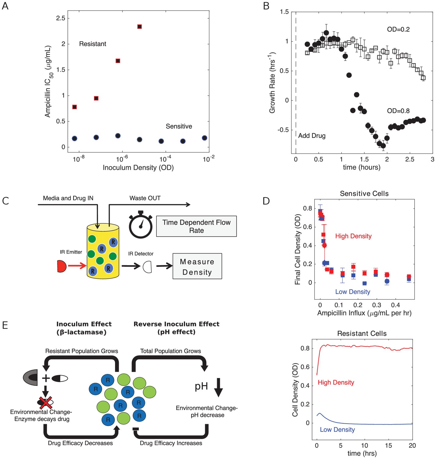
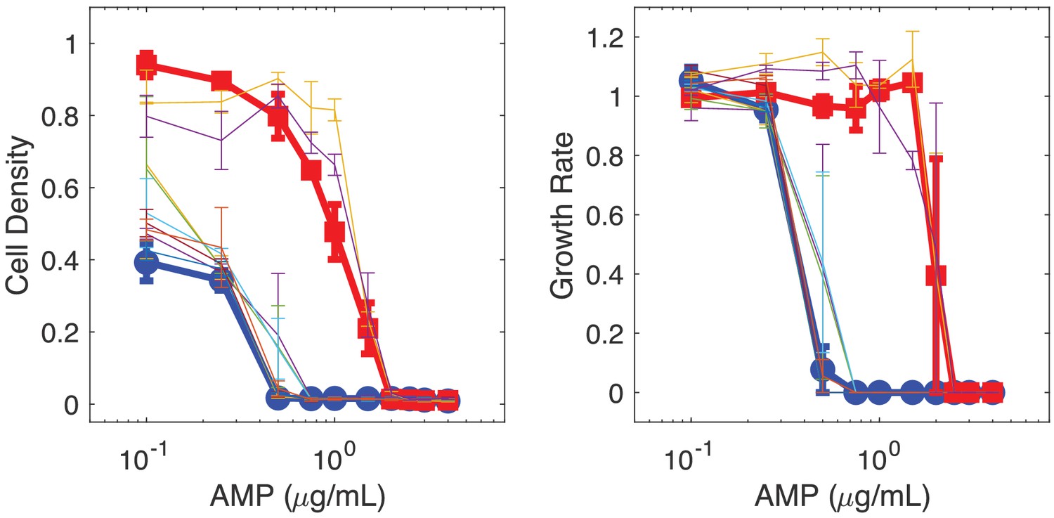
Changes in cell density have opposing effects on β-lactam efficacy in drug sensitive and drug resistant populations.

(A) Half-maximal inhibitory concentration (IC₅₀) of ampicillin as a function of inoculum density for resistant (red squares) and sensitive (blue circles) populations. IC₅₀ is estimated using a fit to Hill-like function $f (x) = {(1 + {(x / K)}^{h})}^{- 1}$ , where $h$ is a Hill coefficient and $K$ is the IC₅₀. (B) Per capita growth rate of drug-sensitive populations held at a density of OD = 0.2 (open squares) and OD = 0.8 (filled circles) following addition of ampicillin at time 0. Growth rate is estimated, as in Karslake et al. (2016), from the average media flow rate required to maintain populations at the specified density in the presence of a constant drug concentration of 0.5 µg/mL. Flow rate is averaged over sliding 20 min windows after drug is added. Note that drug-resistant populations exhibit no growth inhibition over these density ranges, even for drug concentrations in excess of 10³µg/mL. (C) Schematic of experimental setup. Cell density in planktonic populations is measured via light scattering from IR detector/emitter pairs calibrated to optical density (OD). Fresh media (containing appropriate drug concentrations) is introduced over time using computer-controlled peristaltic pumps, and waste is simultaneously removed to maintain constant volume (see Materials and methods). (D) Top panel: final cell density of drug sensitive populations exposed to constant drug influx over a 20 hr period. Experiments were started from either ‘high density’ (OD = 0.6, red) or ‘low density’ (OD = 0.1, blue) initial populations. Bottom panel: cell density time series for drug-resistant populations exposed to ampicillin influx of approximately 1200 µg/mL per hour. In all experiments media was refreshed and waste removed at a rate of µ₀ ≈ 0.1 hr⁻¹. E. In mixed populations containing both sensitive (green) and resistant (blue, ‘R’) cells, there are opposing density-dependent effects on drug efficacy. Increasing the density of resistant cells is expected to decrease drug efficacy as a result of increased β-lactamase production (left side). By contrast, increasing the density of the total cell population decreases the local pH and increases the efficacy of β-lactam antibiotics (right side).

Figure 1—source data 1 Experimental data in Figure 1.: https://cdn.elifesciences.org/articles/52813/elife-52813-fig1-data1-v2.xlsx
Download elife-52813-fig1-data1-v2.xlsx

Figure 2 with 1 supplement

Download asset Open asset

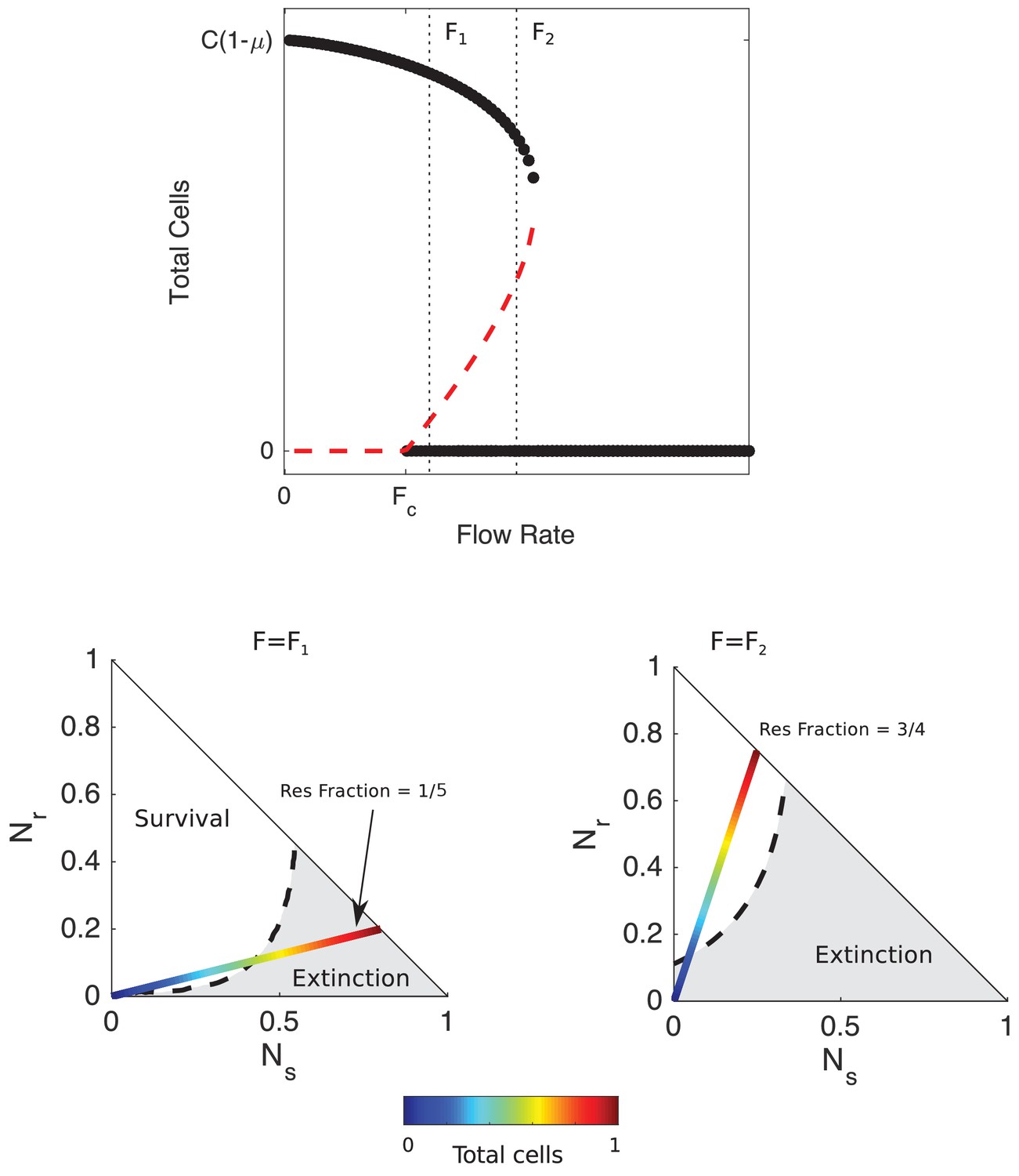
Mathematical model predicts bistability due to opposing density-dependent effects of sensitive and resistant cells on drug inhibition.

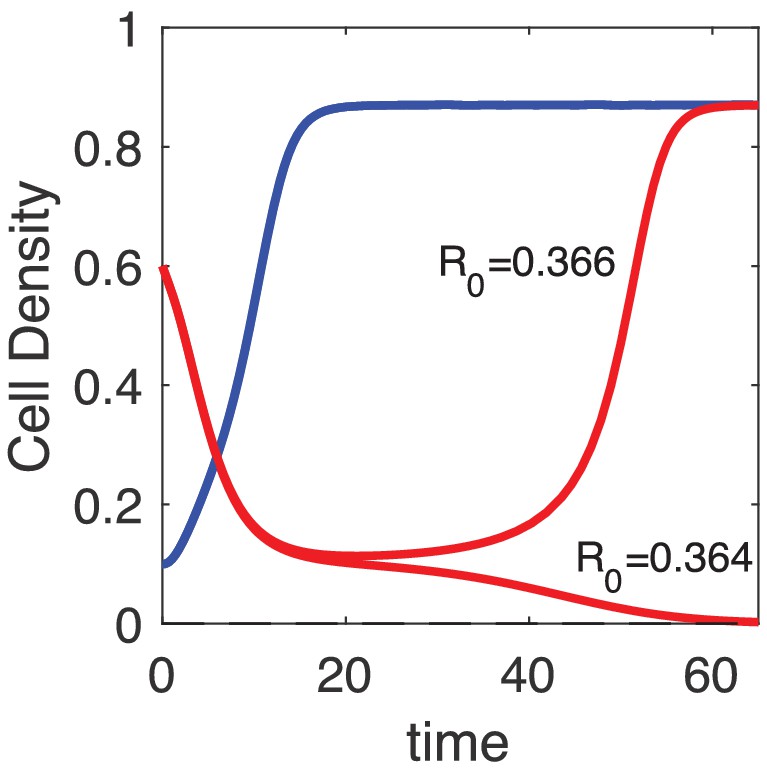
Top: bifurcation diagram showing stable (filled circles) and unstable (red dashed curves) fixed points for different values of drug influx ( $F$ ) and the total number of cells ( $N_{s} + N_{r}$ ). $F_{c} \approx μ K$ is the critical value of drug influx above which the zero solution (extinction) becomes stable; μ is the rate at which cells and drugs are removed from the system (and is measure in units of $g_{m a x}$ , the maximum per capita growth rate of cells in drug-free media, and $K_{r}$ is the factor increase in drug MIC of the resistant strain relative to the wild-type strain. Vertical black dashed lines correspond to $F = F_{1} > F_{c}$ (small drug influx, just above threshold) and $F_{2} ≫ F_{c}$ (large drug influx). Bottom panels: regions of survival (white) and extinction (grey) in the space of sensitive ( $N_{s}$ ) and resistant ( $N_{r}$ ) cells for flow rate $F = F_{1}$ (left) and $F = F_{2}$ (right). Dashed lines show separatrix, the contour separating survival from extinction. Multicolor lines represent constant resistant fractions (1/5, left; 3/4, right) at different total population sizes (ranging from 0 (blue) to a maximum density of 1 (red)). Cell numbers are measured in units of carrying capacity. Specific numerical plots were calculated with $h = 1.4$ , $g_{m i n} = 1 / 3$ , $g_{m a x} = 1$ , $ϵ_{1} = 1.1$ , $ϵ_{2} = 1.5$ , $γ = 0.1$ , $K_{r} = 14$ , $F_{1} = 1.4$ , and $F_{2} = 2.2$ .

Figure 2—figure supplement 1

Download asset Open asset

Separatrix contours separating survival from extinction with and without reverse inoculum effect.

Contour lines separating regions of survival and extinction in the space of sensitive ( $N_{s}$ ) and resistant ( $N_{r}$ ) cells for a series of flow rates (increasing from blue to red) that span the bistable region with (left) and without (right) the reverse inoculum effect. Each contour line shows the separatrix for a particular value of $F$ in the bistable region. For the lowest value of $F$ , the region of extinction is shaded gray while the region of survival is white. Cell numbers are measured in units of carrying capacity. Specific numerical plots were calculated with $h = 1.4$ , $g_{m i n} = 1 / 3$ , $g_{m a x} = 1$ , $ϵ_{2} = 1.5$ , $γ = 0.1$ , $K_{r} = 14$ , and flow rates ranging from $1.4 < F < 2.7$ (left) and $1.4 < F < 7.1$ (right). $ϵ_{1} = - 1.1$ in the left panel and 0 in the right panel. Initial drug concentration is set to 5x MIC of drug-sensitive cells in all panels, though qualitatively similar (but shifted) contours occur for other initial conditions.

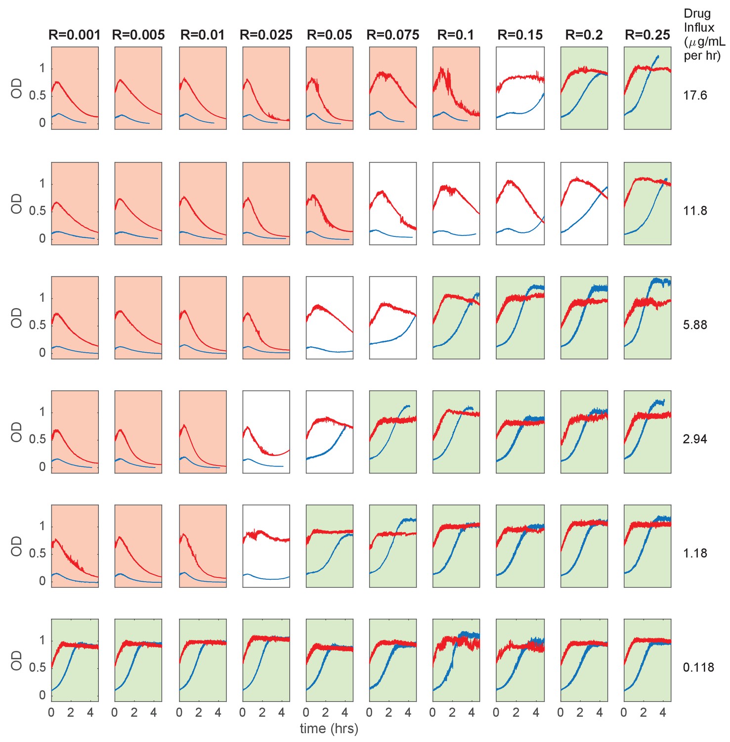
Figure 3 with 8 supplements

Download asset Open asset

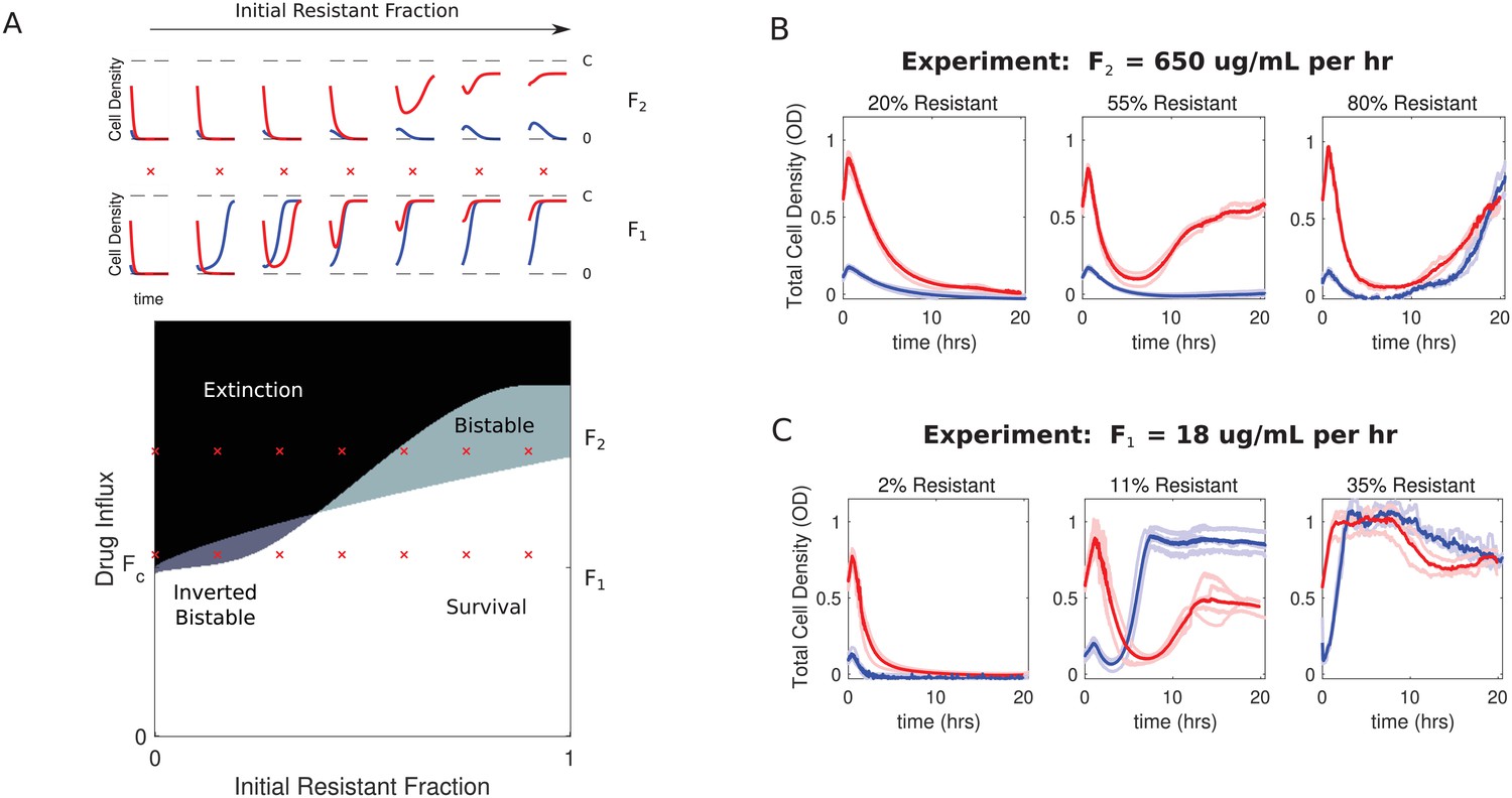
Bistability may favor survival of populations with highest or lowest initial density.

(A) Main panel: phase diagram indicating regions of extinction (black), survival (white), bistability (light gray; initially large population survives, small population dies), and ‘inverted’ bistability (dark gray; initially small population survives, large population dies). Red ’x’ marks correspond to the subplots in the top panels. Top panels: time-dependent population sizes starting from a small population (OD = 0.1, blue) and large population (OD = 0.6, red) at constant drug influx of $F_{2} ≫ F_{c}$ (large drug influx) and $F_{1} > F_{c}$ (small drug influx). $F_{c}$ is the critical influx rate above which the extinct solution (population size 0) first becomes stable; it depends on model parameters, including media refresh rate (µ), maximum kill rate of the antibiotic ( $g_{m i n}$ ), the Hill coefficient of the dose response curve ( $h$ ), and the MIC of the drug-resistant population in the low-density limit where cooperation is negligible ( $K$ ). Specific numerical plots were calculated with $h = 1.4$ , $g_{m i n} = 1 / 3$ , $g_{m a x} = 1$ , $ϵ_{1} = 1.1$ , $ϵ_{2} = 1.5$ , $γ = 0.1$ , $K_{r} = 14$ , $F_{1} = 1.4$ , and $F_{2} = 2.2$ . (B) Experimental time series for mixed populations starting at a total density of OD = 0.1 (blue) or OD = 0.6 (red). The initial populations are comprised of resistant cells at a total population fraction of 0.2 (left), 0.55 (center), and 0.80 right) for influx rate $F_{1} = 650$ µg/mL. Light curves are individual experiments, dark curves are means across all experiments. (C) Experimental time series for mixed populations starting at a total density of OD = 0.1 (blue) or OD = 0.6 (red). The initial populations are comprised of resistant cells at a total population fraction of 0.02 (left), 0.11 (center), and 0.35 right) for influx rate $F_{1} = 18$ µg/mL. Light curves are individual experiments, dark curves are means across all experiments.

Figure 3—source data 1 Experimental data B in Figure 3.: https://cdn.elifesciences.org/articles/52813/elife-52813-fig3-data1-v2.xlsx
Download elife-52813-fig3-data1-v2.xlsx
Figure 3—source data 2 Experimental data C in Figure 3.: https://cdn.elifesciences.org/articles/52813/elife-52813-fig3-data2-v2.xlsx
Download elife-52813-fig3-data2-v2.xlsx

Figure 3—figure supplement 1

Download asset Open asset

Alternative mathematical models exhibit similar qualitative features, including inverted bistability.

Phase diagrams indicating regions of extinction (black), survival (white), bistability (light gray; initially large population survives, small population dies), and ‘inverted’ bistability (dark gray; initially small population survives, large population dies). Specific numerical plots were calculated with $h = 3$ , $g_{m i n} = 1 / 3$ , $g_{m a x} = 1$ , $ϵ_{1} = 1.1$ , $ϵ_{2} = 1.5$ , $γ = 0.1$ , and $K_{r} = 14$ . In the enzyme release model, simulations were run with $χ = 0.1$ (lysed cells degrade drug at 0.1 times the rate of living cells). For simplicity, we also choose $e p s_{3} = 1$ in the pH-IC₅₀ model and $c_{0} = 1$ in the Monod growth model.

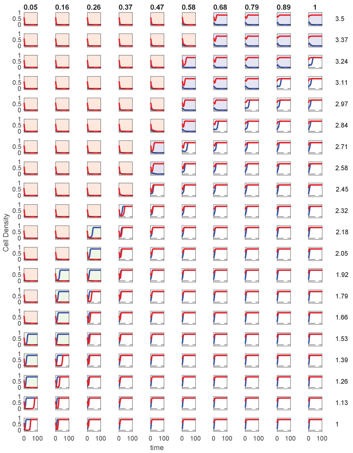
Figure 3—figure supplement 2

Download asset Open asset

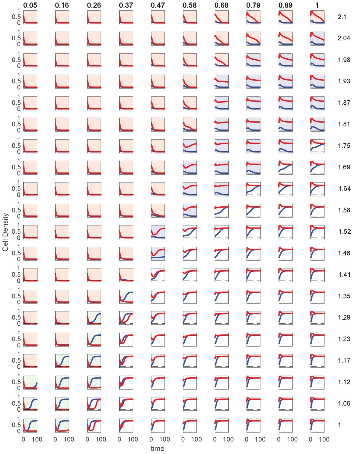
Time series of cell density for simulations starting from high- or low-density populations in Monod growth model.

Time series of cell density for populations starting from a density of 0.6 (red) or 0.1 (blue) for different values of the drug influx rate (different rows) and initial resistant fractions (different columns). Column headings indicate initial resistant fraction; row headings on right indicate drug influx rate. Specific numerical plots were calculated with $h = 3$ , $g_{m i n} = 1 / 3$ , $g_{m a x} = 1$ , $ϵ_{1} = 1.1$ , $ϵ_{2} = 1.5$ , $γ = 0.1$ , and $K_{r} = 14$ . Background color indicates that both populations go extinct (red), both populations survive (white), high-density populations survive while low-density populations go extinct (dark blue; bistable), or high-density populations die while low-density populations survive (green; ‘inverted bistable’).

Figure 3—figure supplement 3

Download asset Open asset

Short experiments to explore parameter space for inverted bistability.

Cell density (OD) time series at various initial resistant fractions (columns) and ampicillin influx rate (rows). Populations were started at OD = 0.1 (blue curves) or OD = 0.6 (red curves). Red shaded plots indicate both populations are near extinction, while green shaded plots indicate that both populations are near carrying capacity at end of experiment (<5 hr).

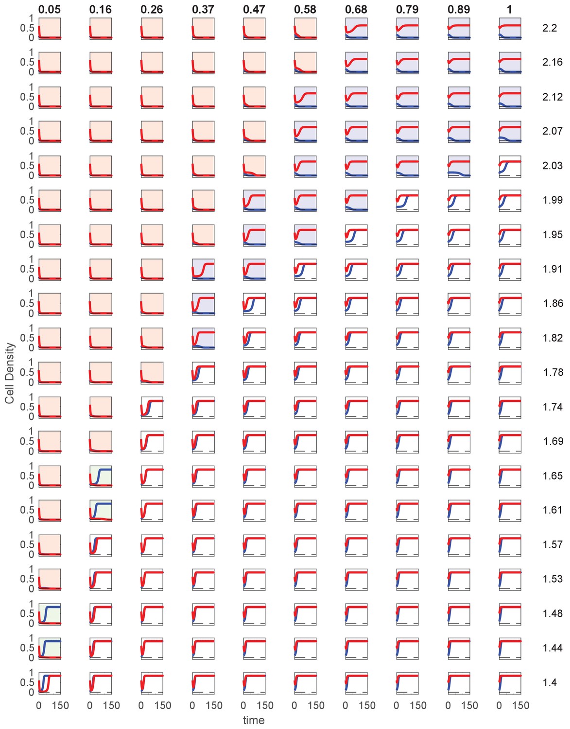
Figure 3—figure supplement 4

Download asset Open asset

Time series of cell density for simulations starting from high- or low-density populations in enzyme release model.

Time series of cell density for populations starting from a density of 0.6 (red) or 0.1 (blue) for different values of the drug influx rate (different rows) and initial resistant fractions (different columns). Column headings indicate initial resistant fraction; row headings on right indicate drug influx rate. Specific numerical plots were calculated with $h = 3$ , $g_{m i n} = 1 / 3$ , $g_{m a x} = 1$ , $ϵ_{1} = 1.1$ , $ϵ_{2} = 1.5$ , $γ = 0.1$ , $χ = 0.1$ , and $K_{r} = 14$ . Background color indicates that both populations go extinct (red), both populations survive (white), high-density populations survive while low-density populations go extinct (dark blue; bistable), or high-density populations die while low-density populations survive (green; ‘inverted bistable’).

Figure 3—figure supplement 5

Download asset Open asset

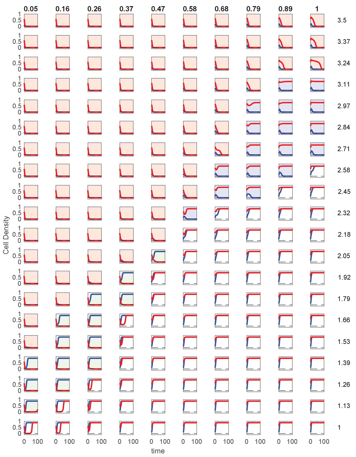
Time series of cell density for simulations starting from high- or low-density populations in pH-IC₅₀ model.

Time series of cell density for populations starting from a density of 0.6 (red) or 0.1 (blue) for different values of the drug influx rate (different rows) and initial resistant fractions (different columns). Column headings indicate initial resistant fraction; row headings on right indicate drug influx rate. Specific numerical plots were calculated with $h = 3$ , $g_{m i n} = 1 / 3$ , $g_{m a x} = 1$ , $ϵ_{2} = 1.5$ , $ϵ_{3} = 1$ , $γ = 0.1$ , and $K_{r} = 14$ . Background color indicates that both populations go extinct (red), both populations survive (white), high-density populations survive while low-density populations go extinct (dark blue; bistable), or high-density populations die while low-density populations survive (green; ‘inverted bistable’).

Figure 3—figure supplement 6

Download asset Open asset

Time series of cell density for simulations starting from high or low-density populations.

Time series of cell density for populations starting from a density of 0.6 (red) or 0.1 (blue) for different values of the drug influx rate (different rows) and initial resistant fractions (different columns). Column headings indicate initial resistant fraction; row headings on right indicate drug influx rate. Specific numerical plots were calculated with $h = 3$ , $g_{m i n} = 1 / 3$ , $g_{m a x} = 1$ , $ϵ_{1} = 1.1$ , $ϵ_{2} = 1.5$ , $γ = 0.1$ , and $K_{r} = 14$ . Background color indicates that both populations go extinct (red), both populations survive (white), high-density populations survive while low density populations go extinct (dark blue; bistable), or high-density populations die while low-density populations survive (green; ‘inverted bistable’).

Figure 3—figure supplement 7

Download asset Open asset

Isolates from populations exhibiting collapse but not complete extinction show similar dose-response behavior as original strains.

Dose response curves illustrate effect of AMP on final cell density (left) and per capita growth rate (right). Bold curves correspond to original sensitive (blue) and resistant (red) strains. Light curves correspond to randomly selected single-colony isolates taken from collapse populations (11% initial resistant fraction; drug influx rate of 18 g/mL; initial density of 0.6; see Figure 3C, middle panel, red curves) at the end of the experiment. Points are mean ± 1 SEM over three technical replicates.

Figure 3—figure supplement 8

Download asset Open asset

Populations exhibit transient periods of approximately constant density near regions of inverted bistability.

Populations starting from a density of 0.6 collapse and exhibit long-lived states of nonzero, nearly-constant density on timescales comparable to or longer than those at which low-density populations reach steady state (in this example, approximately 10 hr). These transient long-lived states ultimately collapse or recover, depending on the specific value of $R_{0}$ (the initial resistant fraction).

Figure 4

Download asset Open asset

Eliminating reverse inoculum effect eliminates inverted bistability.

(A) Numerical phase diagram in absence of reverse inoculum effect ( $ϵ_{1} = 0$ ) indicating regions of extinction (black), survival (white), and bistability (light gray; initially large population survives, small population dies). There are no regions of ‘inverted’ bistability (initially small population survives, large population dies). Red ’x’ marks fall along a line that previously traversed a region of inverted bistability in the presence of a reverse inoculum effect (Figure 3) but includes only surviving populations in its absence. $F_{c}$ is the critical influx rate above which the extinct solution (population size 0) first becomes stable; it depends on model parameters, including media refresh rate (µ), maximum kill rate of the antibiotic ( $g_{m i n}$ ), the Hill coefficient of the dose-response curve ( $h$ ), and the MIC of the drug-resistant population in the low-density limit where cooperation is negligible ( $K$ ). Specific phase diagram was calculated with same parameters as in Figure 3 except $ϵ_{1}$ , which corresponds to the reverse inoculum effect, is set to 0. (B) Experimental time series for mixed populations starting at a total density of OD = 0.1 (blue) or OD = 0.6 (red) in regular media (left panels) or strongly buffered media (right panels). The initial populations are comprised of resistant cells at a total population fraction of 0.11 (top) and 0.15 (bottom) and for influx rate of $F_{1} = 18$ µg/mL. Light curves are individual experiments, dark curves are means across all experiments.

Figure 4—source data 1 Experimental data in Figure 4.: https://cdn.elifesciences.org/articles/52813/elife-52813-fig4-data1-v2.xlsx
Download elife-52813-fig4-data1-v2.xlsx

Figure 5 with 1 supplement

Download asset Open asset

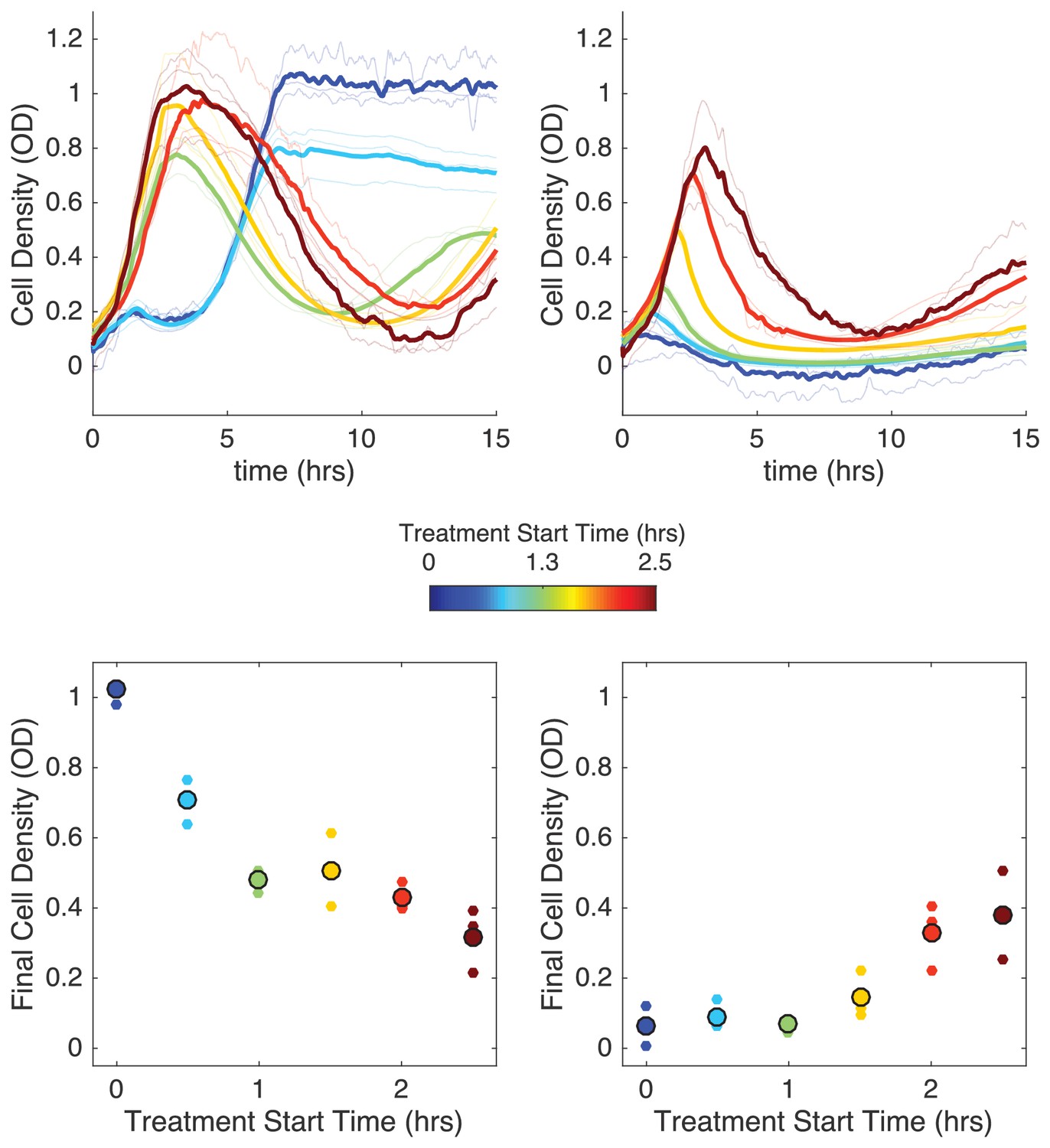
Delaying antibiotic exposure tips populations toward survival or extinction depending on initial resistance fraction and drug influx rate.

Top panels: experimental time series for mixed populations with small initial resistance and low drug influx (left; initial resistance fraction, 0.11 µg/mL) or large initial resistance and high drug influx (right; initial resistance fraction, 0.55 µg/mL). Antibiotic influx was started immediately (blue) or following a delay of up to 2.5 hr (dark red). Light transparent lines are individual replicates; dark lines are means over replicates. In experiments with nonzero delays, antibiotic influx was replaced by influx of drug-free media during the delay. Bottom panels: final cell density (15 hr) as a function of delay (‘treatment start time’). small points are individual replicates; large circles are means across replicates.

Figure 5—source data 1 Experimental data in Figure 5.: https://cdn.elifesciences.org/articles/52813/elife-52813-fig5-data1-v2.xlsx
Download elife-52813-fig5-data1-v2.xlsx

Figure 5—figure supplement 1

Download asset Open asset

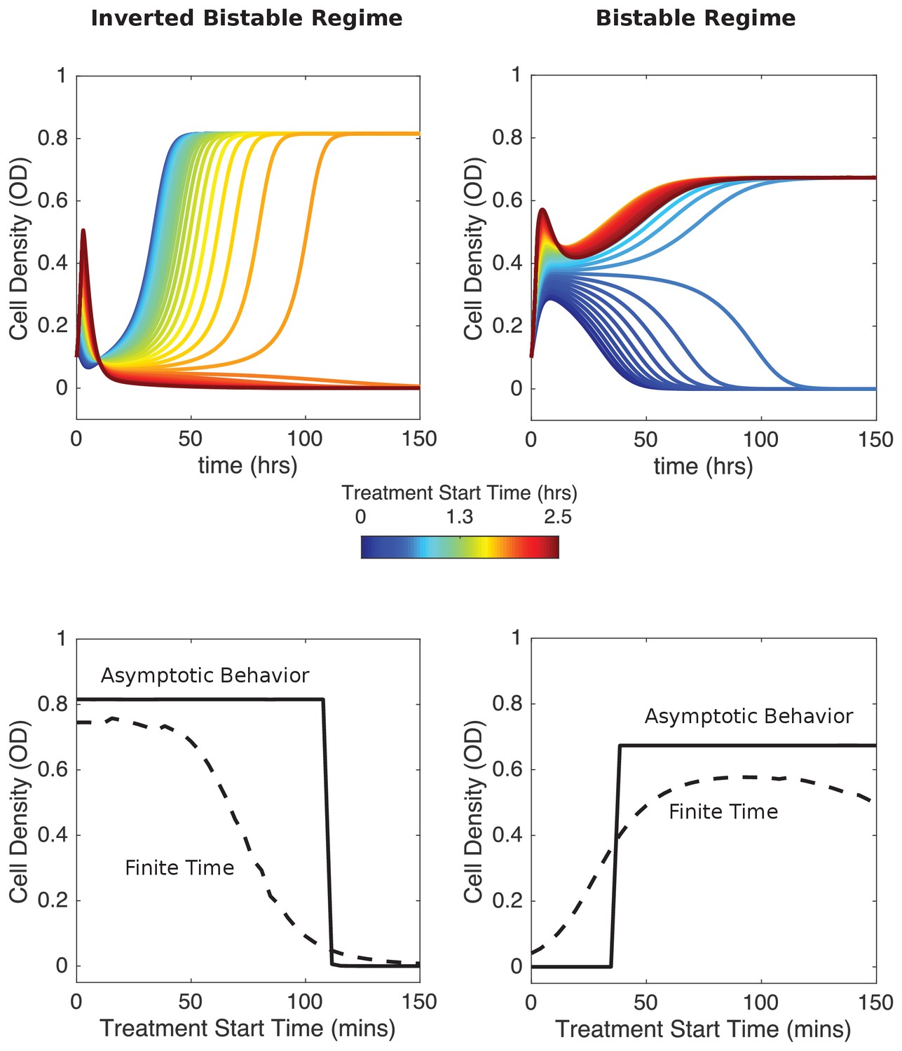
Numerical results indicate that delaying antibiotic exposure tips populations toward survival or extinction depending on initial resistance fraction and drug influx rate.

Top panels: time series for mixed populations with small initial resistance and low drug influx (left; initial resistance fraction, 0.04) or large small initial resistance and high drug influx (right; initial resistance fraction, 0.56). Antibiotic influx was started immediately (blue) or following a delay of up to 2.5 hr (dark red). Bottom panels: final cell density at finite times (40 hr, dashed curves) or asymptotically long times (150 hr; solid curves) as a function of delay (‘treatment start time’). Model parameters are the same as those used in Figure 2.

Tables

Key resources table

Reagent (species)	Designation	Source	Additional info
Gene (E. faecalis )	β-lactamase	Zscheck and Murray, 1991; Rice et al. (1991); Rice and Marshall (1992)	PCR from strain CH19
Gtrain (E. faecalis )	OG1RF	Dunny et al. (1978); Oliver et al. (1977)
Plasmid	pBSU101-DasherGFP	Aymanns et al. (2011); Hallinen et al. (2019)	Reporter plasmid
Plasmid	pBSU101-BFP-BL	Hallinen et al. (2019), this paper	Expresses β-lactamase
Drug	Spectinomcyin sulfate	MP Biomedicals	CAT 0215899302
Drug	Ampicillin Sodium Salt	Fisher	CAT BP1760-25

Additional files

Transparent reporting form: https://cdn.elifesciences.org/articles/52813/elife-52813-transrepform-v2.docx
Download elife-52813-transrepform-v2.docx

Download links

A two-part list of links to download the article, or parts of the article, in various formats.

Downloads (link to download the article as PDF)

Open citations (links to open the citations from this article in various online reference manager services)

Mendeley

Cite this article (links to download the citations from this article in formats compatible with various reference manager tools)

Kelsey M Hallinen
Jason Karslake
Kevin B Wood

(2020)

Delayed antibiotic exposure induces population collapse in enterococcal communities with drug-resistant subpopulations

eLife 9:e52813.

https://doi.org/10.7554/eLife.52813

Share this article

Cite this article

Changes in cell density have opposing effects on β-lactam efficacy in drug sensitive and drug resistant populations.

Figure 1—source data 1

Mathematical model predicts bistability due to opposing density-dependent effects of sensitive and resistant cells on drug inhibition.

Separatrix contours separating survival from extinction with and without reverse inoculum effect.

Bistability may favor survival of populations with highest or lowest initial density.

Figure 3—source data 1

Figure 3—source data 2

Alternative mathematical models exhibit similar qualitative features, including inverted bistability.

Time series of cell density for simulations starting from high- or low-density populations in Monod growth model.

Short experiments to explore parameter space for inverted bistability.

Time series of cell density for simulations starting from high- or low-density populations in enzyme release model.

Time series of cell density for simulations starting from high- or low-density populations in pH-IC50 model.

Time series of cell density for simulations starting from high or low-density populations.

Isolates from populations exhibiting collapse but not complete extinction show similar dose-response behavior as original strains.

Populations exhibit transient periods of approximately constant density near regions of inverted bistability.

Eliminating reverse inoculum effect eliminates inverted bistability.

Figure 4—source data 1

Delaying antibiotic exposure tips populations toward survival or extinction depending on initial resistance fraction and drug influx rate.

Figure 5—source data 1

Numerical results indicate that delaying antibiotic exposure tips populations toward survival or extinction depending on initial resistance fraction and drug influx rate.

Transparent reporting form

Downloads (link to download the article as PDF)

Open citations (links to open the citations from this article in various online reference manager services)

Cite this article (links to download the citations from this article in formats compatible with various reference manager tools)

Time series of cell density for simulations starting from high- or low-density populations in pH-IC₅₀ model.