Network dynamics underlying OFF responses in the auditory cortex
- Laboratoire de Neurosciences Cognitives et Computationelles, Département d’études cognitives, ENS, PSL University, INSERM, France
- Neural Computation Laboratory, Center for Human Technologies, Istituto Italiano di Tecnologia (IIT), Italy
- Départment de Neurosciences Intégratives et Computationelles (ICN), Institut des Neurosciences Paris-Saclay (NeuroPSI), UMR 9197 CNRS, Université Paris Sud, France
- Institut Pasteur, INSERM, Institut de l’Audition, France
Figures
Figure 1
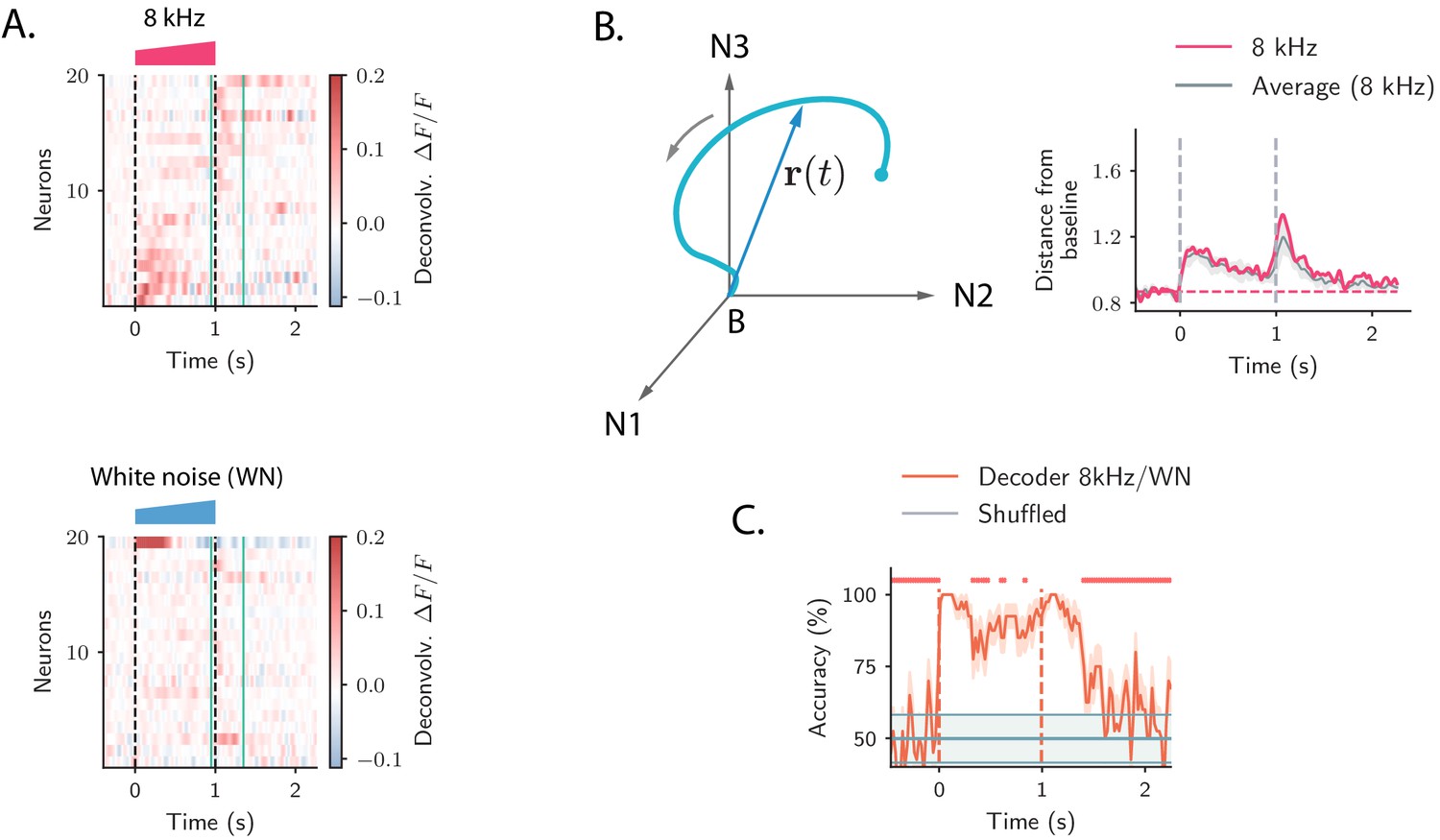
Strong transient ON and OFF responses in auditory cortex of mice passively listening to different sounds.
(A) Top: deconvolved calcium signals averaged over 20 trials showing the activity (estimated firing rate) of 20 out of 2343 neurons in response to a 8 kHz 1 s UP-ramp with intensity range 60–85 dB. We selected neurons with high signal-to-noise ratios (ratio between the peak activity during ON/OFF responses and the standard deviation of the activity before stimulus presentation). Neurons were ordered according to the difference between peak activity during ON and OFF response epochs. Bottom: activity of the same neurons as in the top panel in response to a white noise (WN) sound with the same duration and intensity profile. In all panels dashed lines indicate onset and offset of the stimulus, and green solid lines show the temporal region where OFF responses were analyzed (from 50 ms before stimulus offset to 300 ms after stimulus offset). (B) Left: cartoon showing the OFF response to one stimulus as a neural trajectory in the state space, where each coordinate represents the firing rate of one neuron (with respect to the baseline B). The length of the dashed line represents the distance between the population activity vector and its baseline firing rate, that is, . Right: the red trace shows the distance from baseline computed for the population response to the 8 kHz sound in A. The gray trace shows the distance from baseline averaged over the 8 kHz sounds of 1 s duration (four stimuli). The gray shading represents ±1 standard deviation. The dashed horizontal line shows the average level of the distance before stimulus presentation (even if baseline-subtracted responses were used, a value of the norm different from zero is expected because of noise in the spontaneous activity before stimulus onset). (C) Accuracy of stimulus classification between a 8 kHz versus WN UP-ramping sounds over time based on single trials (20 trials). The decoder is computed at each time step (spaced by ∼50 ms) and accuracy is computed using leave-one-out cross-validation. Orange trace: average classification accuracy over the cross-validation folds. Orange shaded area corresponds to ±1 standard error. The same process is repeated after shuffling stimulus labels across trials at each time step (chance level). Chance level is represented by the gray trace and shading, corresponding to its average and ±1 std computed over time. The red markers on the top indicate the time points where the average classification accuracy is lower than the average accuracy during the ON transient response (, two-tailed t-test).
Figure 2 with 4 supplements
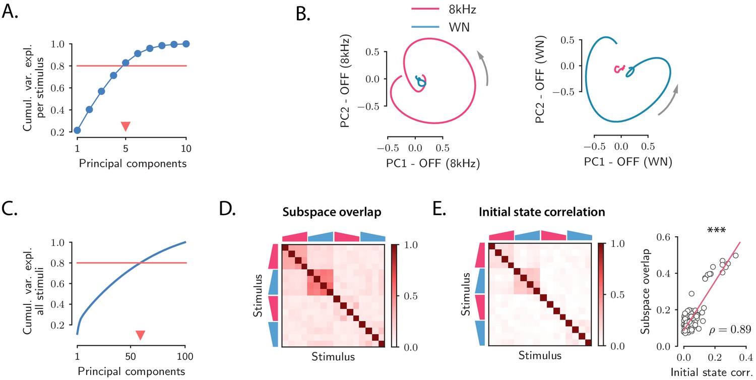
Low-dimensional structure of population OFF responses.
(A) Cumulative variance explained for OFF responses to individual stimuli, as a function of the number of principal components. The blue trace shows the cumulative variance averaged across all 16 stimuli. Error bars are smaller than the symbol size. The triangular marker indicates the number of PCs explaining 80% (red line) of the total response variance for individual stimuli. (B) Left: projection of the population OFF response to the 8 kHz and white noise (WN) sounds on the first two principal components computed for the OFF response to the 8 kHz sound. Right: projection of both responses onto the first two principal components computed for the OFF response to the WN sound. PCA was performed on the period from −50 ms to 300 ms with respect to stimulus offset. We plot the response from 50 ms before stimulus offset to the end of the trial duration. (C) Cumulative variance explained for the OFF responses to all 16 stimuli together as a function of the number of principal components. The triangular marker indicates the number of PCs explaining 80% of the total response variance for all stimuli. (D) Overlap between the subspaces defined by the first five principal components of the OFF responses corresponding to pairs of stimuli. The overlap is measured by the cosine of the principal angle between these subspaces (see Materials and methods, Section 'Correlations between OFF response subspaces'). (E) Left: correlation matrix between the initial population activity states at the end of stimulus presentation (50 ms before offset) for each pair of stimuli. Right: linear correlation between subspace overlaps (D) and the overlap between initial states (E left panel) for each stimulus pair. The component of the dynamics along the corresponding initial states was subtracted before computing the subspace overlaps.
Figure 2—figure supplement 1
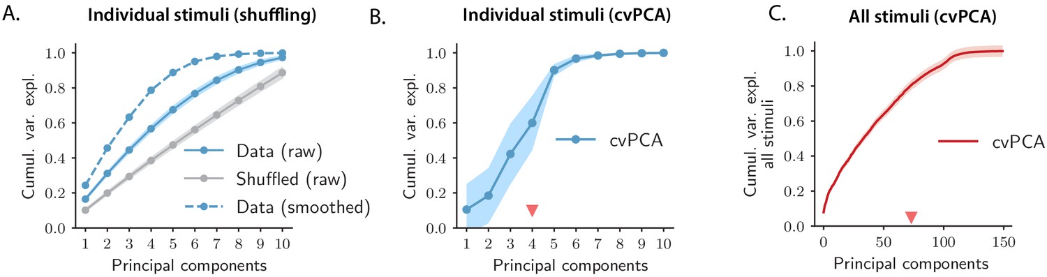
Controls for PCA of OFF responses to individual stimuli and across stimuli.
(A) Solid blue trace: cumulative variance explained for population OFF responses to individual stimuli evaluated using PCA on raw calcium traces (13 data points). Gray trace: cumulative variance explained after shuffling cell indices independently at each time step to remove temporal correlations between time points. Responses where the temporal correlations have been removed exhibit higher dimensionality with respect to the original responses. For comparison, the cumulative variance explained computed on the temporally smoothed responses (see Materials and methods, Section 'Principal component analysis') is shown (dashed blue trace). (B) Cumulative variance explained evaluated using the cross-validated PCA (cvPCA) method (Stringer et al., 2019) applied to the OFF responses to individual stimuli. For each stimulus we evaluated the cvPCA spectrum averaging over all pairs of trials extracted from 20 total trials (see Materials and methods, Section 'Cross-validated PCA'). The solid trace and color shading represent the mean and standard deviation of the cumulative variance over stimuli. (C) Cumulative variance explained evaluated using the cvPCA method applied to the OFF responses to all stimuli at once. Here the solid trace and color shading represent the mean and standard error of the cumulative variance computed over all pairs of trials. In both plots the triangular red markers indicate the cvPCA dimensionalities that explain at least 80% of the response variance.
Figure 2—figure supplement 2
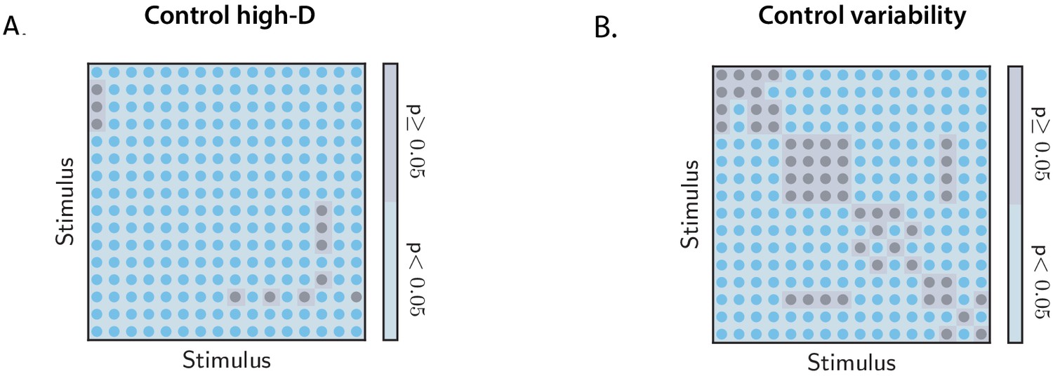
Controls for the orthogonality between OFF response subspaces.
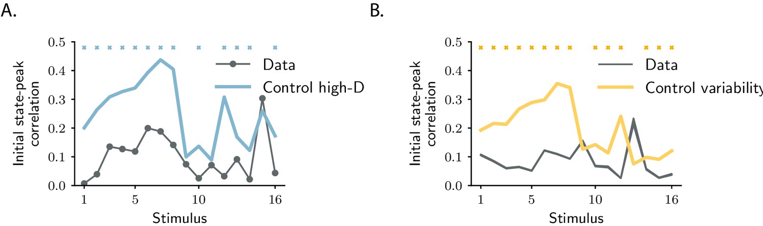
(A) Statistical control testing for the hypothesis that small subspace overlaps are due to the high dimensionality of neural responses. Blue and gray regions indicate stimulus pairs for which the p-value for the difference between the data and the controls is respectively smaller and larger or equal than 0.05 (lower tail test). Blue regions therefore indicate the stimulus pairs for which low values of the subspace overlaps are not attributable to the high dimensionality of the state-space. The number of shuffles is set to 200 (see Materials and methods, Section 'Controls for subspace overlaps and initial state-peak correlations'). (B) Statistical control testing for the hypothesis that small subspace overlaps are due to the trial-to-trial variability of neural responses. Blue and gray regions indicate stimulus pairs for which the p-value for the difference between the data and the controls is respectively smaller and larger or equal than 0.05 (two-tailed independent t-test). Blue regions therefore indicate the stimulus pairs for which low values of the subspace overlaps are not attributable to the trial-to-trial variability of neural activity. The number of trial subsamplings is set to 200 (see Materials and methods, Section 'Controls for subspace overlaps and initial state-peak correlations').
Figure 2—figure supplement 3

Relation between ON and OFF responses in the auditory cortex.
(A) Left: projection of the population ON and OFF responses to a 8 kHz pure tone (1 s, UP-ramp, with intensity range 60–85 dB) on the first two principal components computed on the ON response. Right: projection of both ON and OFF responses to the same stimulus on the first two principal components computed on the OFF response. PCA was performed on the period from −50 ms to 300 ms with respect to stimulus onset and offset. (B) Subspace overlaps between the subspaces spanned by the ON and OFF population responses to individual stimuli. The subspace overlap is computed as the cosine of the principal angle between the ON and OFF subspaces, defined by the first five principal components of the ON and OFF population responses respectively. Error bars correspond to ±1 standard deviations computed over 100 subsamplings of the 80% of the units. (C) Projection of the population response for the stimulus in A, along the population activity vector at the peak of the transient ON and OFF responses (corresponding to the maximum distance from baseline).
Figure 2—figure supplement 4

Overlap between the states at the peak of the transient OFF responses.
(A) Left: overlap between the states at the peak of the OFF responses for each pair of stimuli. The peak time is defined as the time at which the distance from baseline of the population vector is maximum. Right: linear correlation between the overlaps between peak states and the overlaps between initial conditions for each stimulus pair. (B) Same as A except that, for each stimulus, the component of the peak state along the corresponding initial condition has been subtracted.
Figure 3 with 3 supplements
Comparison between single-cell and network models for OFF response generation.
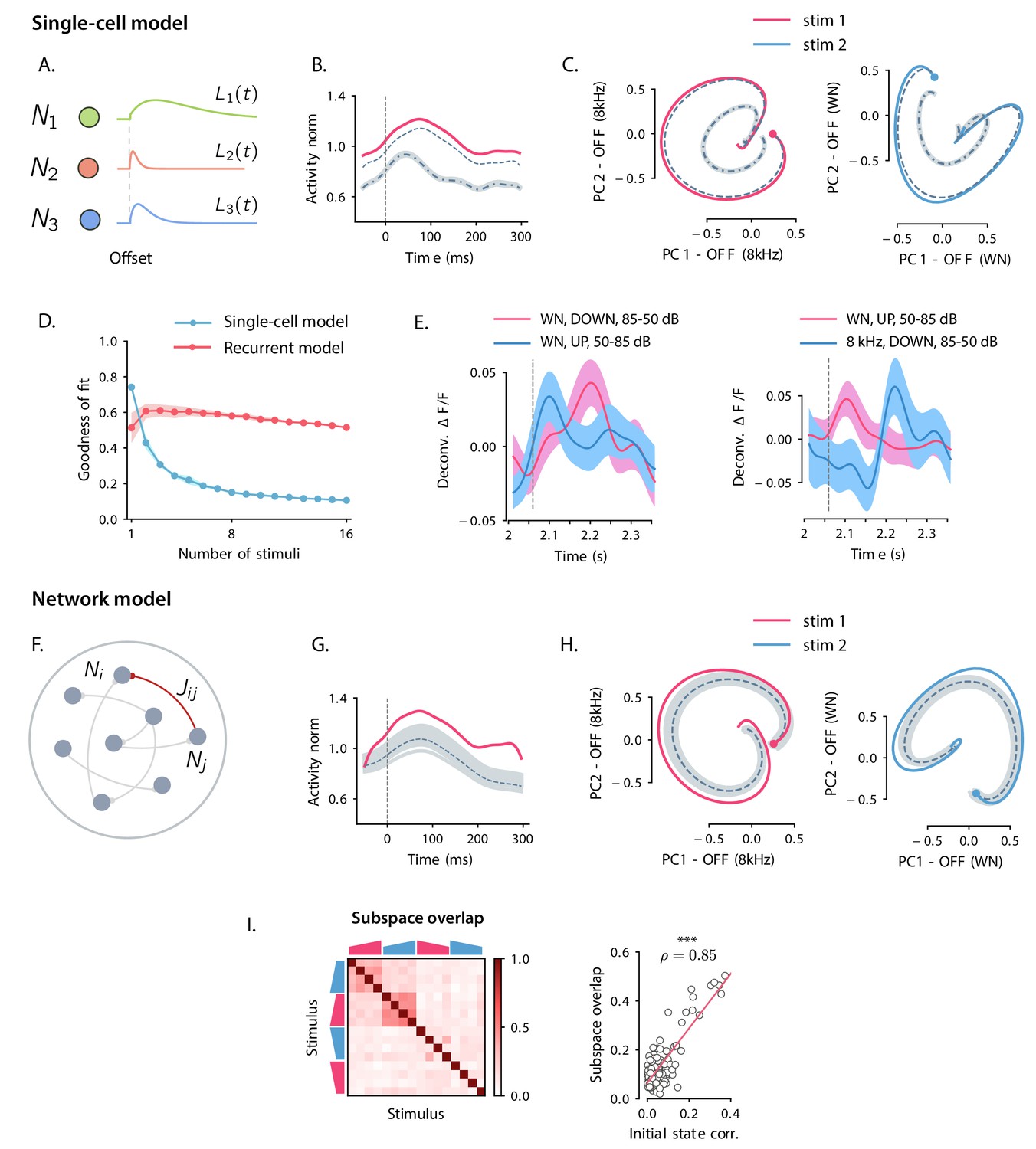
(A) Cartoon illustrating the single-cell model defined in Equation (1). The activity of each unit is described by a characteristic temporal response (colored traces). Across stimuli, only the relative activation of the single units changes, while the temporal shape of the responses of each unit does not vary. (B) Distance from baseline of the population activity vector during the OFF response to one example stimulus (red trace; same stimulus as in C left panel). The dashed vertical line indicates the time of stimulus offset. Gray dashed lines correspond to the norms of the population activity vectors obtained from fitting the single-cell model respectively to the OFF response to a single stimulus (dashed line), and simultaneously to the OFF responses to two stimuli (dash-dotted line; in this example, the two fitted stimuli are the ones considered in panel C). In light gray we plot the norm of 100 realizations of the fitted OFF response by simulating different initial states distributed in the vicinity of the fitted initial state (shown only for the simultaneous fit of two stimuli for clarity). Note that in the single-cell model fit (see Materials and methods, Section 'Fitting the single-cell model'), the fitted initial condition can substantially deviate from the initial condition taken from the data. (C) Colored traces: projection of the population OFF responses to two distinct example stimuli (same stimuli as in Figure 2B) onto the first two principal components of either stimulus. As in panel B gray dashed and dash-dotted traces correspond to the projection of the OFF responses obtained when fitting the single-cell model to one or two stimuli at once. (D) Goodness of fit (as quantified by coefficient of determination ) computed by fitting the single-cell model (blue trace) and the network model (red trace) to the calcium activity data, as a function of the number of stimuli included in the fit. Both traces show the cross-validated value of the goodness of fit (10-fold cross-validation in the time domain). Error bars represent the standard deviation over multiple subsamplings of a fixed number of stimuli (reported on the abscissa). Prior to fitting, for each subsampling of stimuli, we reduced the dimensionality of the responses using PCA, and kept the dominant dimensions that accounted for 90% of the variance. (E) Examples of the OFF responses to distinct stimuli of two different auditory cortical neurons (each panel corresponds to a different neuron). The same neuron exhibits different temporal response profiles for different stimuli, a feature consistent with the network model (see Figure 6A,D), but not with the single-cell model. (F) Illustration of the recurrent network model. The variables defining the state of the network are the (baseline-subtracted) firing rates of the units, denoted by . The strength of the connection from unit j to unit i is denoted by . (G) Distance from baseline of the population activity vector during the OFF response to one example stimulus (red trace; same stimulus as in C left panel). Gray traces correspond to the norms of the population activity vectors obtained from fitting the network model to the OFF response to a single stimulus and generated using the fitted connectivity matrix. The initial conditions were chosen in a neighborhood of the population activity vector 50 ms before sound offset. 100 traces corresponding to 100 random choices of the initial condition are shown. Dashed trace: average distance from baseline. (H) Colored traces: projection of the population OFF responses to two different stimuli (same stimuli as in Figure 2B) on the first two principal components. Gray traces: projections of multiple trajectories generated by the network model using the connectivity matrix fitted to the individual stimuli as in G. The initial condition is indicated with a dot. 100 traces are shown. Dashed trace: projection of the average trajectory. (I) Left: overlap between the subspaces corresponding to OFF response trajectories to pairs of stimuli (as in Figure 2D) generated using the connectivity matrix fitted to all stimuli at once. Right: linear correlation between subspace overlaps and the overlaps between the initial states for each stimulus pair computed using the trajectories obtained by the fitted network model. The component of the dynamics along the corresponding initial states was subtracted before computing the subspace overlaps.
Figure 3—figure supplement 1
Goodness of fit for the network and single-cell models adjusted for the number of parameters.
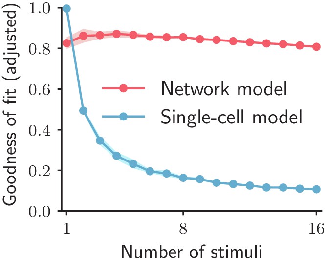
Goodness of fit, as quantified by coefficient of determination adjusted for the numbers of parameters, when fitting the single-cell model (blue trace) and the network model (red trace) to the calcium activity data, as a function of the number of stimuli included in the fit. Both traces show the cross-validated value of the goodness of fit (10-fold cross-validation in the time domain). Error bars represent the standard deviation over multiple subsamplings of a fixed number of stimuli (on the abscissa). Prior to fitting, for each subsampling of stimuli, we reduced the dimensionality of the responses using PCA, and kept the dominant dimensions accounting for 90% of the variance.
Figure 3—figure supplement 2
Goodness of fit for the original and surrogate data sets.
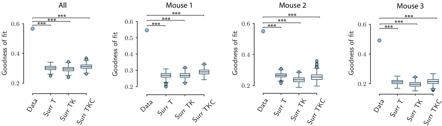
Value of the goodness of fit for the network model (as quantified by the coefficient of determination ) for the original data sets and for three types of surrogate data sets, computed using the activity pooled across the three animals (All) and the activity of individual animals (mouse 1, 2, and 3). For the original data set, the dot shows the goodness of fit averaged over the cross-validation. For the surrogate data sets, the average goodness of fit over cross-validation folds is shown for multiple (n=500) surrogates of the original data. The network model fits significantly better the original data than all three types of surrogate data sets (*** corresponds to p<0.001; upper tail test using the value of the goodness of fit averaged over the cross-validations folds for each data set). Box-and-whisker plots show the distribution of the values for the three types of surrogates (Tukey convention: box lower end, middle line, and upper end represent the first quartile, median, and third quartile of the distributions; lower and upper whisker extends for 1.5 times the interquartile range). Fitting is performed on the population OFF responses to all 16 stimuli at once. The goodness of fit is computed using 10-fold cross-validation in the time domain. The parameters for the reduced-rank ridge regression for the three plots are respectively: , and , , .
Figure 3—figure supplement 3
Goodness of fit as a function of PC dimensionality for original and surrogate data sets.
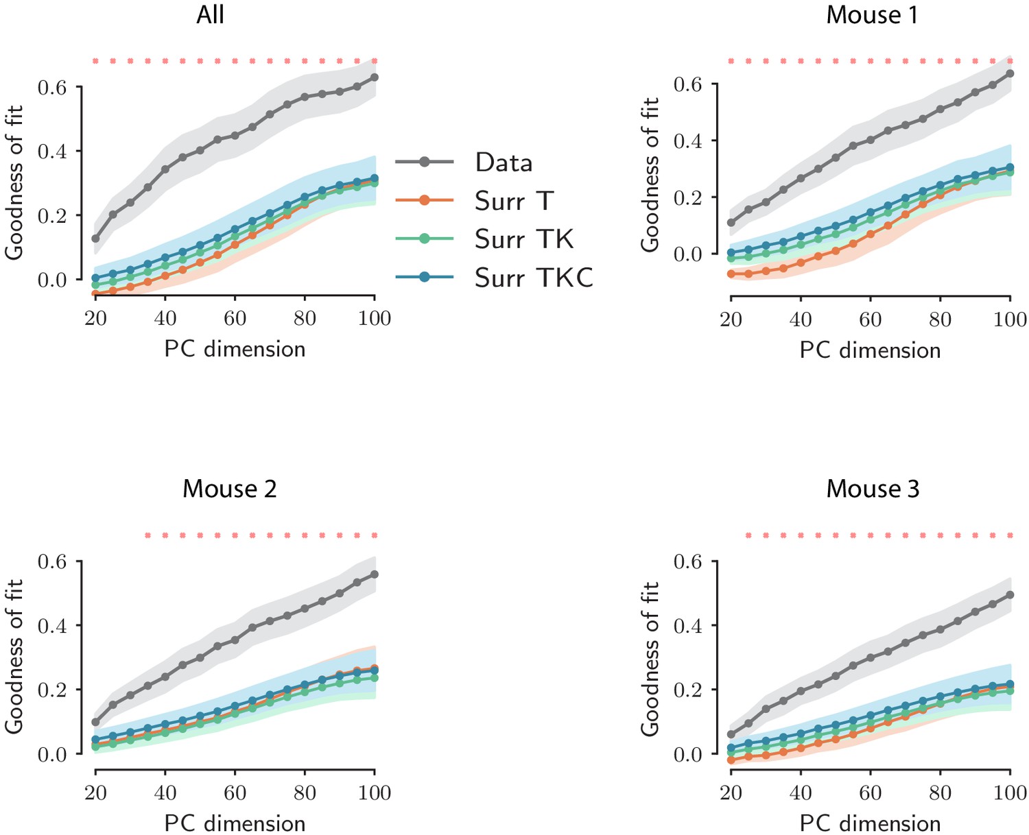
Value of the goodness of fit as a function of PC dimensionality for the original data set (black trace) and for the surrogate data sets (colored traces). The value of the goodness of fit was computed using ridge regression using 10-fold cross-validation. The ridge parameter is optimized for each choice of the PC dimensionality. For the original data set, error bars represent the standard error over the 10 cross-validation folds; for the surrogate data sets, error bars represent the average cross-validation standard error over all the surrogates. Here the number of surrogates is set to 100. For each choice of the PC dimensionality, red crosses indicate that the difference in goodness of fit between the original data set and the most constraining surrogate (TKC) is statistically significant (p<0.01; upper tail test using the mean value of the goodness of fit over the cross-validation folds for each data set).
Figure 4
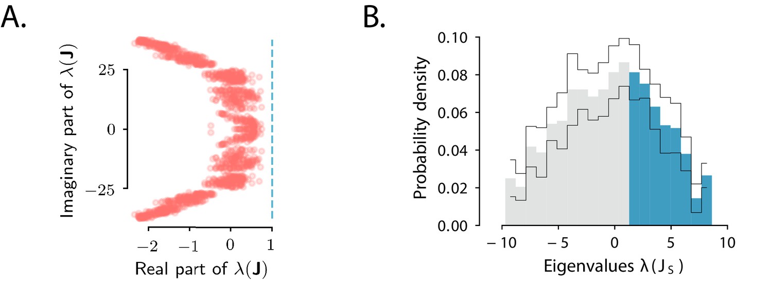
Spectra of the connectivity matrix of the fitted network model.
(A) Eigenvalues of the connectivity matrix obtained by fitting the network model to the population OFF responses to all 1 s stimuli at once. The dashed line marks the stability boundary given by . (B) Probability density distribution of the eigenvalues of the symmetric part of the effective connectivity, . Eigenvalues larger than unity (; highlighted in blue) determine strongly non-normal dynamics. In A and B the total dimensionality of the responses was set to 100. The fitting was performed on 20 bootstrap subsamplings (with replacement) of 80% of neurons out of the total population. Each bootstrap subsampling resulted in a set of 100 eigenvalues. In panel A we plotted the eigenvalues of obtained across all subsamplings. In panel B the thin black lines indicate the standard deviation of the eigenvalue probability density across subsamplings. In panels A and B, the temporal window considered for the fit was extended from 350 ms to 600 ms, to include the decay to zero baseline of the OFF responses. The extension of the temporal window was possible only for the 1 s long stimuli (n=8), since the length of the temporal window following stimulus offset for the 2 s stimuli was limited by the length of the neural recordings.
Figure 5 with 3 supplements

Low-dimensional structure of the dynamics of OFF responses to individual stimuli.
(A) Goodness of fit (coefficient of determination) as a function of the rank of the fitted network, normalized by the goodness of fit computed using ordinary least squares ridge regression. The shaded area represents the standard deviation across individual stimuli. For reduced-rank regression captures more than 80% (red solid line) of the variance explained by ordinary least squares regression. (B) Left: overlap matrix consisting of the overlaps between left and right connectivity patterns of the connectivity fitted on one example stimulus. The color code shows strong (and opposite in sign) correlation values between left and right connectivity patterns within pairs of nearby modes. Weak coupling is instead present between different rank-2 channels (highlighted by dark boxes). Right: histogram of the absolute values of the correlation between right and left connectivity patterns, across all stimuli, and across 20 random subsamplings of 80% of the neurons in the population for each stimulus. Left and right connectivity vectors are weakly correlated, except for the pairs corresponding to the off-diagonal couplings within each rank-2 channel. The two markers indicate the average values of the correlations within each group. When fitting individual stimuli the rank parameter and the number of principal components are set respectively to 6 and 100. (C) Left: absolute value of the difference between and (see panel B) divided by 2, across stimuli. For a rank-R channel (here ) comprising rank-2 channels, the maximum difference across the rank-2 channels is considered. Large values of this difference indicate that the dynamics of the corresponding rank-R channel are amplified. Right: component of the initial state on the left connectivity vectors , (i.e. in Equation (75)), obtained from the fitted connectivity to individual stimuli (in green). The component of the initial condition along the left connectivity vectors (green box) is larger than the component of random vectors along the same vectors (gray box). In both panels the boxplots show the distributions across all stimuli of the corresponding average values over 20 random subsamplings of 80% of the neurons. The rank parameter and the number of principal components are the same as in B. (D) For each stimulus, we show the correlation between the state at the end of stimulus presentation and the state at the peak of the OFF response, defined as the time of maximum distance from baseline. Error bars represent the standard deviation computed over 2000 bootstrap subsamplings of 50% of the neurons in the population (2343 neurons). (E) Correlation between initial state and peak state obtained from fitting the single-cell (in green) and network models (in red) to a progressively increasing number of stimuli. For each fitted response the peak state is defined as the population vector at the time of maximum distance from baseline of the original response. The colored shaded areas correspond to the standard error over 100 subsamplings of a fixed number of stimuli (reported on the abscissa) out of 16 stimuli. For each subsampling of stimuli, the correlation is computed for one random stimulus.
Figure 5—figure supplement 1
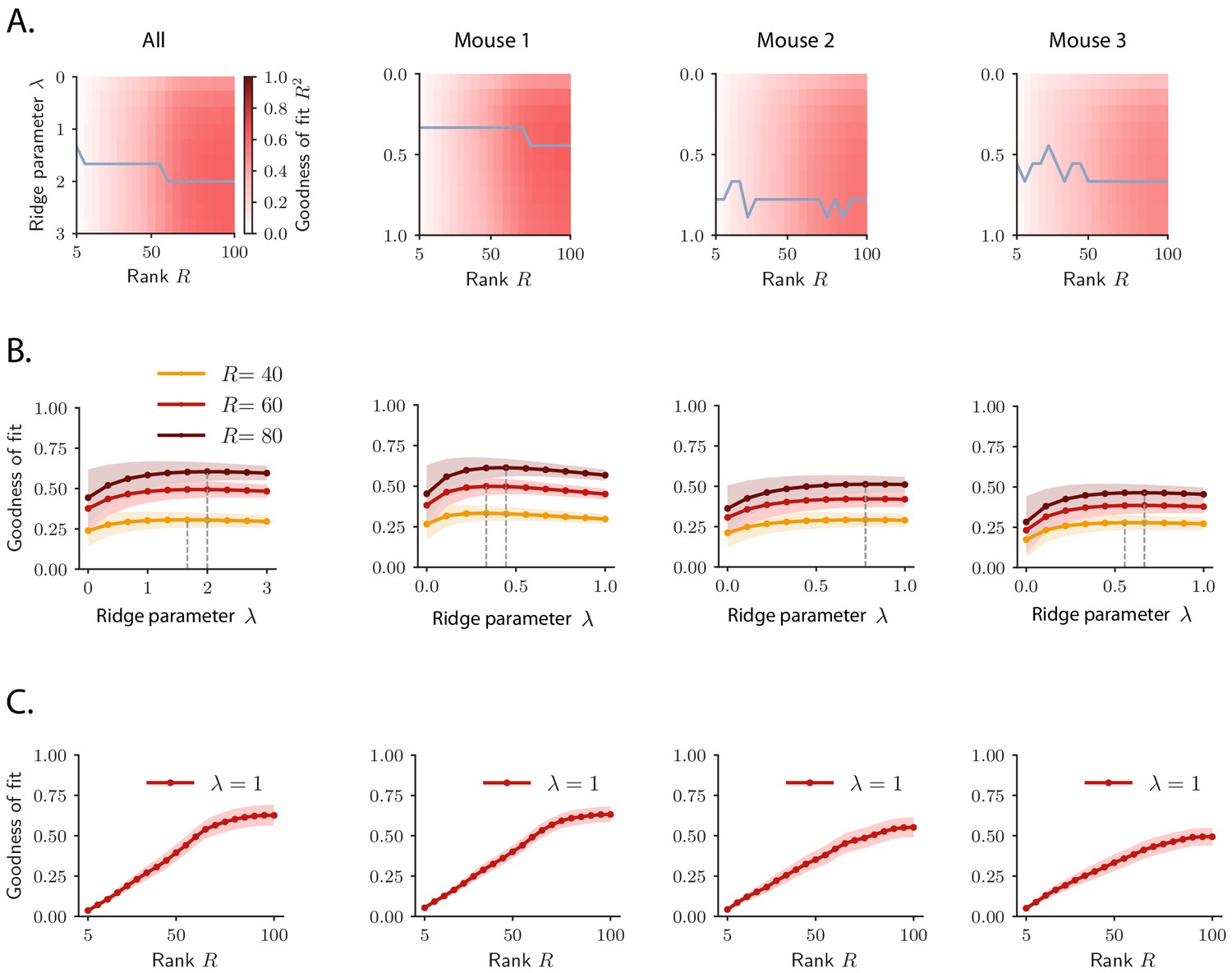
Selection of hyperparameters in rank-reduced ridge regression.
The ridge and rank hyperparameters and are selected using 10-fold cross-validation in the time domain, when fitting the activity of the whole pseudopopulation (All) or the activity of individual animals (mouse 1, 2, and 3). (A) Goodness of fit as a function of the hyperparameters and . The gray trace shows the value of for which the goodness of fit is maximum for each value of the rank parameter . (B) Goodness of fit as a function of the hyperparameters for three different choices of the rank . The value of for which the goodness of fit is maximum is indicated by the dashed line. (C) Goodness of fit as a function of the rank for . The value of the goodness of fit as a function of the rank does not exhibit a clear maximum, but rather tends to saturate at a certain value of the rank .
Figure 5—figure supplement 2
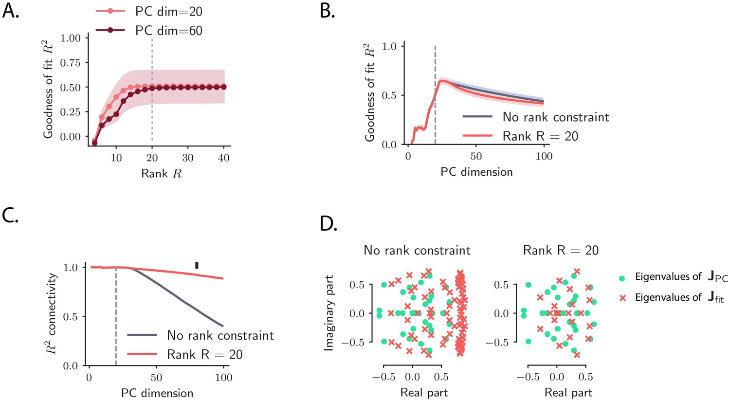
Model recovery for simulated OFF responses using a low-rank network model.
Model recovery for OFF responses generated through a low-rank network model. The number of units was set to . The connectivity matrix consisted of orthogonal transient channels, each one with rank equal to one, given by , where all the left and right connectivity vectors are mutually orthogonal (). We generated 10 OFF responses by setting the initial state of the network to 10 orthogonal left connectivity vectors . Input noise was injected into the system. Thus, the dynamics across stimuli spanned at least 20 dimensions. (A) Goodness of fit as a function of the rank parameter in the reduced-rank regression fit, for two values of the PC dimensionality. Ten-fold cross-validation is used; error bars represent the standard error across the 10 cross-validation folds. The goodness of fit increases as a function of the rank and stays approximately constant for values of the rank bigger or equal to 20 (dashed line). (B) Goodness of fit as a function of the PC dimensionality computed using ordinary least square regression (with no rank constraint, gray trace) and reduced-rank regression (with , red trace). The dashed line indicated the number of dimensions spanned by the dynamics for all stimuli in case of zero input noise (equal to 20 in this case). For a value of the PC dimensionality larger than the number of dimensions spanned by the dynamics, the goodness of fit decreases due to overfitting. Cross-validation is performed as in A. (C) Similarity, as quantified by the coefficient of determination , between the elements of connectivity resulting from the fitting procedure and the projection of the real connectivity on the top principal components, i.e. (where contains as columns the principal components), as a function of the number of principal components considered. The gray trace corresponds to ordinary least square regression, while the red trace to reduced-rank regression with rank . (D) Spectra of the matrices (green dots) and (red crosses) using ordinary least square regression (left) and reduced-rank regression (right) for fixed dimensionality (equal to 80, black marker in panel C). In all panels, the ridge parameter is set to .
Figure 5—figure supplement 3
Controls for the orthogonality between initial and peak state.
(A) Statistical control testing for the hypothesis that small correlations are due to the high dimensionality of neural responses. The dark trace represents the absolute value of the correlation between initial and peak state for individual stimuli. The blue trace represents the correlations between initial and peak state after shuffling the labels ‘initial state’ and ‘peak state’ across trials (mean and standard error across shuffles is shown). Blue markers indicate stimulus indices for which the p-value for the difference between the data and the controls is smaller than 0.05 (lower tail test), where a low value of the correlation is not attributable to the high dimensionality of the state-space (see Materials and methods, Section 'Controls for subspace overlaps and initial state-peak correlations'). The number of shuffles is set to 1000. (B) Statistical control testing for the hypothesis that small correlations are due to the trial-to-trial variability of neural responses. The dark trace represents absolute value of the correlation between initial and peak state for individual stimuli (mean and standard error over 1000 subsampling of 10 trials are shown). The yellow trace represents the correlations between responses at the same time points but averaged over two different sets of trials (mean and standard error over 1000 permutations of trials are shown). Yellow markers indicate stimulus indices for which the p-value for the difference between the data and the controls is smaller than 0.05 (two-tailed independent t-test), where a low value of the correlation is not attributable to the trial-to-trial variability of neural responses (see Materials and methods, Section 'Controls for subspace overlaps and initial state-peak correlations').
Figure 6
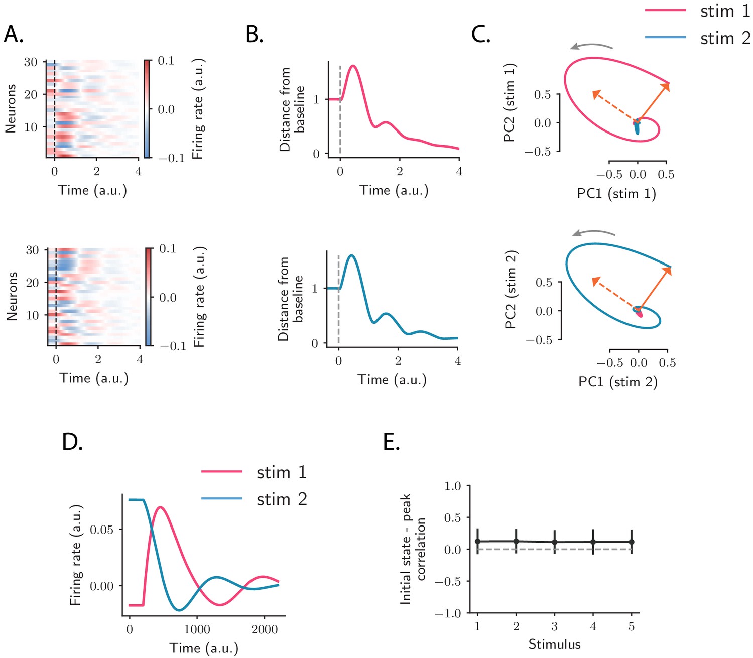
Population OFF responses in a network model with low-rank rotational structure.
(A) Single-unit OFF responses to two distinct stimuli generated by orthogonal rank-2 rotational channels (see Materials and methods, Section 'Dynamics of a low-rank rotational channel'). The two stimuli were modeled as two different activity states and at the end of stimulus presentation (). We simulated a network of 1000 units. The connectivity consisted of the sum of rank-2 rotational channels of the form given by Equation (5, 6) ( in Equation (6) and , for all ). Here the two stimuli were chosen along two orthogonal vectors and . Dashed lines indicate the time of stimulus offset. (B) Distance from baseline of the population activity vector during the OFF responses to the two stimuli in A. For each stimulus, the amplitude of the offset responses (quantified by the peak value of the distance from baseline) is controlled by the difference between the lengths of the right connectivity vectors of each rank-2 channel, that is, . (C) Projection of the population OFF responses to the two stimuli onto the first two principal components of either stimuli. The projections of the vectors and (resp. and ) on the subspace defined by the first two principal components of stimulus 1 (resp. 2) are shown respectively as solid and dashed arrows. The subspaces defined by the vector pairs , and , are mutually orthogonal, so that the OFF responses to stimuli 1 and 2 evolve in orthogonal dimensions. (D) Firing rate of one example neuron in response to two distinct stimuli: in the recurrent network model the time course of the activity of one unit is not necessarily the same across stimuli. (E) Correlation between the initial state (i.e. the state at the end of stimulus presentation) and the state at the peak of the OFF responses, for five example stimuli. Error bars represent the standard deviation computed over 100 bootstrap subsamplings of 50% of the units in the population.
Figure 7
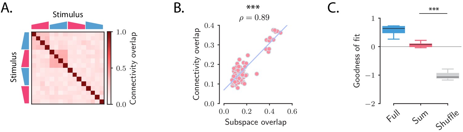
Structure of the transient channels across stimuli.
(A) Overlaps between the transient channels corresponding to individual stimuli (connectivity overlaps), as quantified by the overlap between the right connectivity vectors of the connectivities fitted to each individual stimulus s (see Materials and methods, Section 'Analysis of the transient channels'). The ridge and rank parameters, and the number of principal components have been respectively set to , and (the choice of maximized the coefficient of determination between the connectivity overlaps, A, and the subspace overlaps, Figure 2D). (B) Scatterplot showing the relationship between the subspace overlaps (see Figure 2D) and connectivity overlaps (panel A) for each pair of stimuli. (C) Goodness of fit computed by predicting the population OFF responses using the connectivity (Full) or the connectivity given by the sum of the individual channels (Sum). These values are compared with the goodness of fit obtained by shuffling the elements of the matrix (Shuffle). Box-and-whisker plots show the distributions of the goodness of fit computed for each cross-validation partition (10-fold). For the ridge and rank parameters, and the number of principal components were set to , and (Figure 5—figure supplement 1).
Figure 8
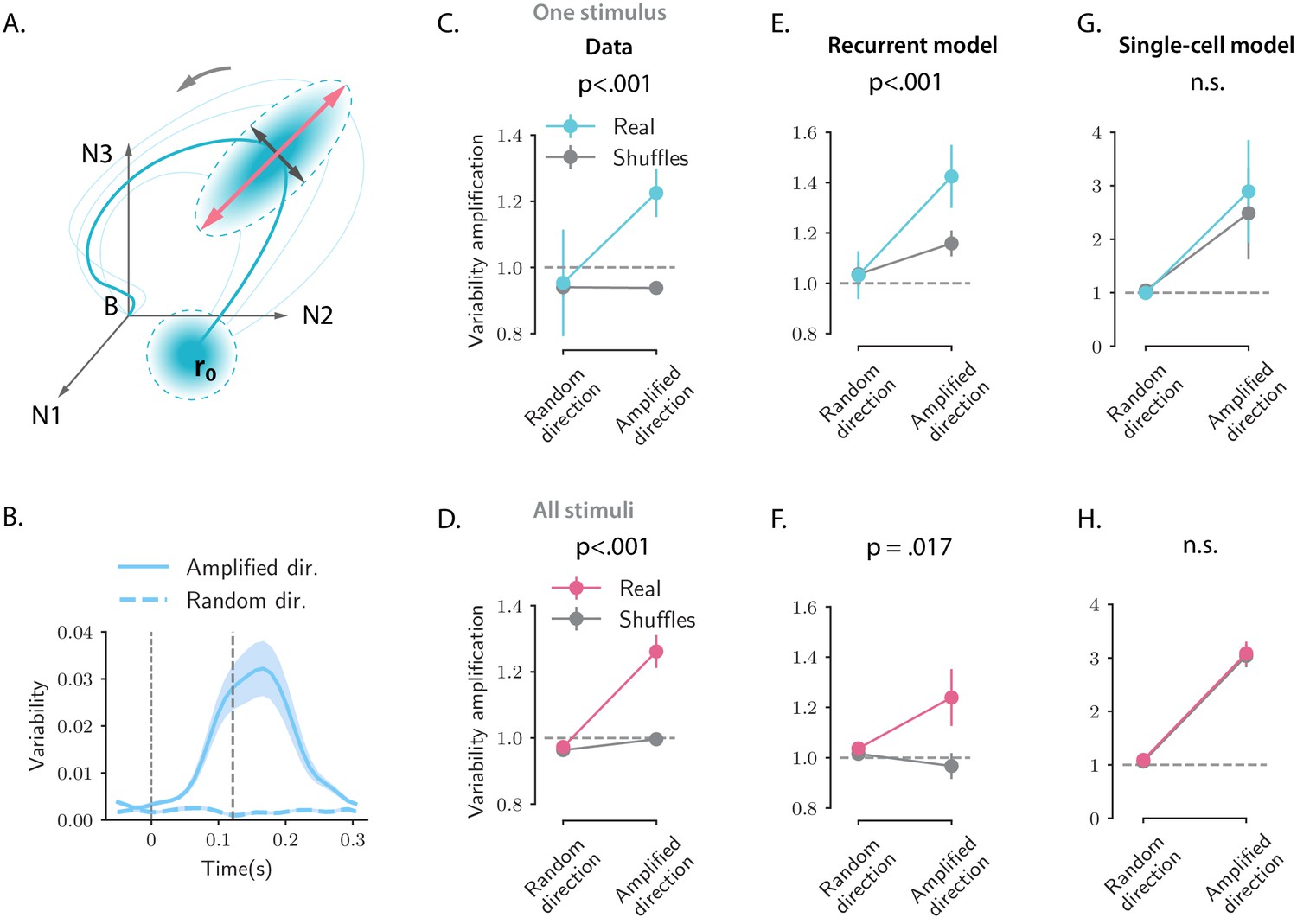
Structure of trial-to-trial variability generated by the network and single-cell models, compared to the auditory cortical data.
(A) Cartoon illustrating the structure of single-trial population responses along different directions in the state-space. The thick and thin blue lines represent respectively the trial-averaged and single-trial responses. Single-trial responses start in the vicinity of the trial-averaged activity . Both the network and single-cell mechanisms dynamically shape the structure of the single-trial responses, here represented as graded blue ellipses. The red and black lines represent respectively the amplified and random directions considered in the analyses. (B) Time course of the variability computed along the amplified direction (solid trace) and along a random direction (dashed trace) for one example stimulus and one example session (287 simultaneously recorded neurons). In this and all the subsequent panels the amplified direction is defined as the population activity vector at the time when the norm of the trial-averaged activity of the pseudo-population pooled over sessions and animals reaches its maximum value (thick dashed line). Thin dashed lines denote stimulus offset. Shaded areas correspond to the standard deviation computed over 20 bootstrap subsamplings of 19 trials out of 20. (C, E, and G) Variability amplification (VA) computed for the amplified and random directions on the calcium activity data (panel C), on trajectories generated using the network model (panel E) and the single-cell model (panel G); (see Materials and methods, Section 'Single-trial analysis of population OFF responses'), for one example stimulus (same as in B). The network and single-cell models were first fitted to the trial-averaged responses to individual stimuli, independently across all recordings sessions (13 sessions, 180 ± 72 neurons). 100 single-trial responses were then generated by simulating the fitted models on 100 initial conditions drawn from a random distribution with mean and covariance matrix equal to the covariance matrix computed from the single-trial initial states of the original responses (across neurons for the single-cell model, across PC dimensions for the recurrent model). Results did not change by drawing the initial conditions from a distribution with mean and isotropic covariance matrix (i.e. proportional to the identity matrix, as assumed for the theoretical analysis in Materials and methods, Section 'Single-trial analysis of population OFF responses'). In the three panels, the values of VA were computed over 50 subsamplings of 90% of the cells (or PC dimensions for the recurrent model) and 50 shuffles. Error bars represent the standard deviation over multiple subsamplings, after averaging over all sessions and shuffles. Significance levels were evaluated by first computing the difference in VA between amplified and random directions () and then computing the p-value on the difference between and across subsamplings (two-sided independent t-test). For the network model, the VA is higher for the amplified direction than for a random direction, and this effect is significantly stronger for the real than for the shuffled responses. Instead, for the single-cell model the values of the VA computed on the real responses are not significantly different from the ones computed on the shuffled responses. (D, F, and H) Values of the VA computed as in panels C, E, and G pooled across all 16 stimuli. Error bars represent the standard error across stimuli. Significance levels were evaluated computing the p-value on the difference between and across stimuli (two-sided Wilcoxon signed-rank test). The fits of the network and single-cell models of panels E, G, F, and H were generated using ridge regression ( for both models).
Scheme 1
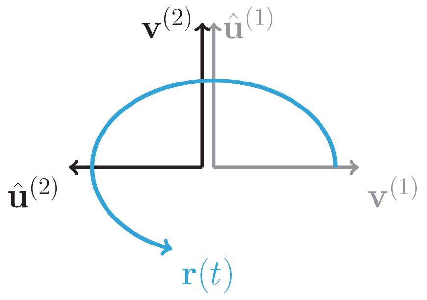
Schematics of the rank-2 rotational channel.
Tables
Table 1
Stimuli set.
| Stimulus | Direction | Frequency | Duration (s) | Modulation (dB) |
|---|---|---|---|---|
| 1 | UP | 8 kHz | 1 s | 50–85 |
| 2 | UP | 8 kHz | 1 s | 60–85 |
| 3 | UP | 8 kHz | 2 s | 50–85 |
| 4 | UP | 8 kHz | 2 s | 60–85 |
| 5 | UP | WN | 1 s | 50–85 |
| 6 | UP | WN | 1 s | 60–85 |
| 7 | UP | WN | 2 s | 50–85 |
| 8 | UP | WN | 2 s | 60–85 |
| 9 | DOWN | 8 kHz | 1 s | 85–50 |
| 10 | DOWN | 8 kHz | 1 s | 85–60 |
| 11 | DOWN | 8 kHz | 2 s | 85–50 |
| 12 | DOWN | 8 kHz | 2 s | 85–60 |
| 13 | DOWN | WN | 1 s | 85–50 |
| 14 | DOWN | WN | 1 s | 85–60 |
| 15 | DOWN | WN | 2 s | 85–50 |
| 16 | DOWN | WN | 2 s | 85–60 |
Additional files
Download links
A two-part list of links to download the article, or parts of the article, in various formats.
Downloads (link to download the article as PDF)
Open citations (links to open the citations from this article in various online reference manager services)
Cite this article (links to download the citations from this article in formats compatible with various reference manager tools)
Network dynamics underlying OFF responses in the auditory cortex
eLife 10:e53151.
https://doi.org/10.7554/eLife.53151


