Figures and data in Quantitative analysis of 1300-nm three-photon calcium imaging in the mouse brain

Figures
Tables
Additional files

3 figures, 5 tables and 2 additional files

Figures

Figure 1 with 1 supplement

Download asset Open asset

Comparison of the power attenuation of 1320 nm and 920 nm excitation light and their respective 3-photon and 2-photon excitation efficiency in the mouse brain.

(A) Power attenuation of 920 nm and 1320 nm excitation light in the mouse brain. The mouse brain vasculature was *uniformly* labeled with fluorescein dextran and imaged *simultaneously* by 920 nm 2PM and 1320 nm 3PM at precisely the same location. The fraction of excitation power reaching the focus from the brain surface (Focus Power/Surface Power) was calculated based on the attenuation of 2PE and 3PE signal with the imaging depth (Materials and methods). (B) The pulse energy required at the brain surface to generate the *same* 2PE and 3PE signal strength (0.1 signal photon detected per laser pulse) at different imaging depths, measured in fluorescein-labeled blood vessels (n = 1 shown) and GCaMP6s-labeled neurons (CamKII-tTA/tetO-GCaMP6s; n = 5 mice). The signal strength is scaled to 60 fs pulse duration for both 2PE and 3PE.

Figure 1—source data 1 A typical power attenuation with depth curve of 1320 nm and 920 nm excitation light in the mouse brain, plotted in Figure 1A.: https://cdn.elifesciences.org/articles/53205/elife-53205-fig1-data1-v2.csv
Download elife-53205-fig1-data1-v2.csv
Figure 1—source data 2 The excitation pulse energy at the brain surface required to generate 0.1 signal photon per pulse at different depths in the mouse brain, measured in fluorescein-labeled vasculature and plotted in Figure 1B.: https://cdn.elifesciences.org/articles/53205/elife-53205-fig1-data2-v2.csv
Download elife-53205-fig1-data2-v2.csv
Figure 1—source data 3 The excitation pulse energy at the brain surface required to generate 0.1 signal photon per pulse at different depths in the mouse brain, measured in the neurons of transgenic animals (CamKII-tTA/tetO-GCaMP6s) and plotted in Figure 1B.: https://cdn.elifesciences.org/articles/53205/elife-53205-fig1-data3-v2.csv
Download elife-53205-fig1-data3-v2.csv

Figure 1—figure supplement 1

Download asset Open asset

Additional power attenuation curves of 920 nm and 1320 nm excitation light in the mouse neocortex (n = 3, >12 weeks old mice, all males).

Figure 1—figure supplement 1—source data 1 Additional power attenuation with depth curves of 1320 nm and 920 nm excitation light in the mouse neocortex, plotted in Figure 1—figure supplement 1.: https://cdn.elifesciences.org/articles/53205/elife-53205-fig1-figsupp1-data1-v2.xlsx
Download elife-53205-fig1-figsupp1-data1-v2.xlsx

Figure 2 with 2 supplements

Download asset Open asset

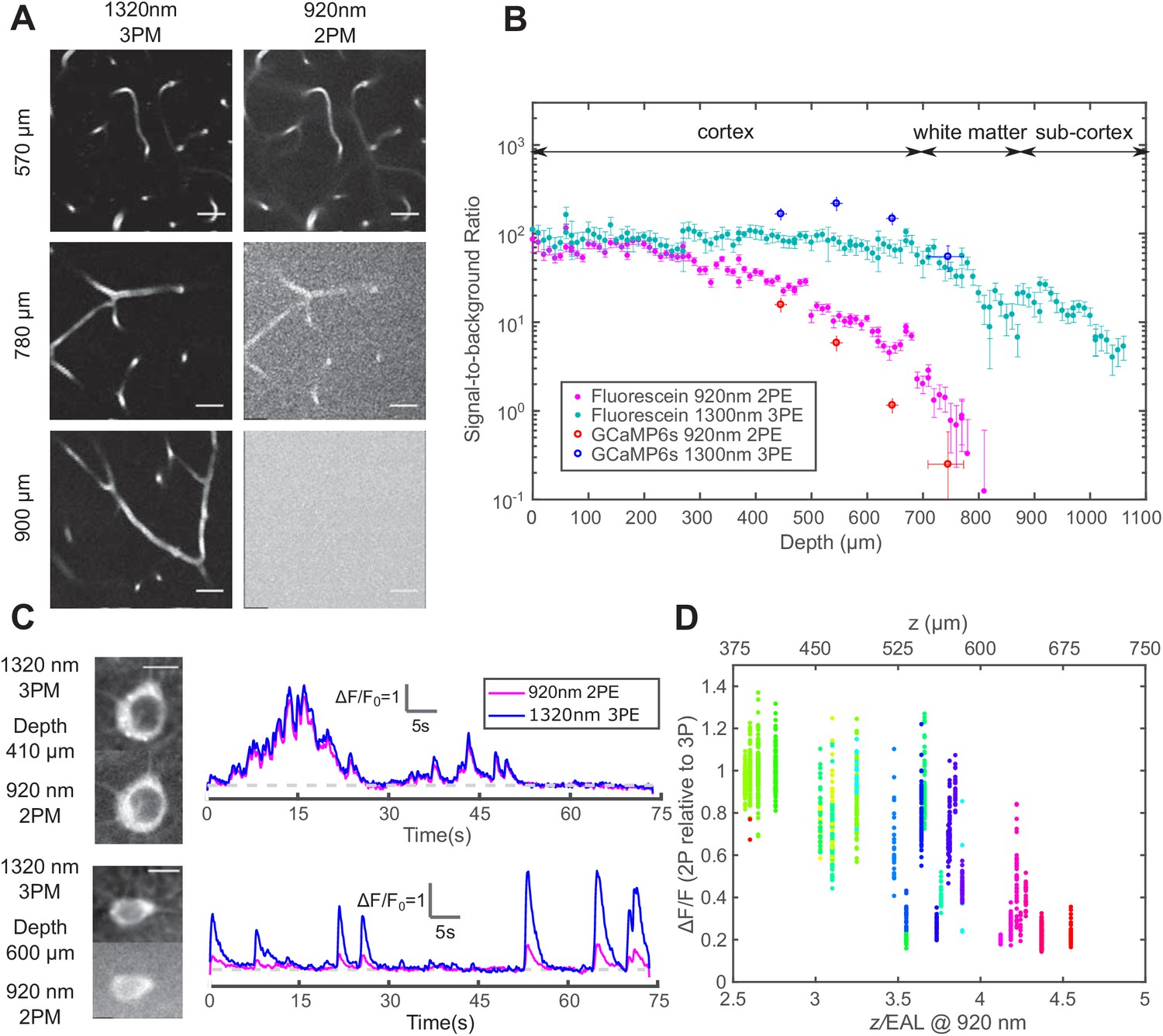
Comparison of signal-to-background ratio for 1320 nm 3PM and 920 nm 2PM in the non-sparsely labeled mouse brain and its effect on calcium imaging sensitivity.

(A) Comparison of 3PM and 2PM images of fluorescein-labeled blood vessels at different depths. Scale bar 30 μm. (B) SBR measured *simultaneously* by 1320 nm 3PE and 920 nm 2PE on fluorescein-labeled blood vessels and GCaMP6s-labeled neurons. Each set of 3PE and 2PE comparison was performed in the same mouse. All vertical error bars denote the standard deviation of SBR caused by feature brightness variation, and horizontal error bars represent the depth range of the measurement. (C) Images and corresponding calcium traces of a cortical L4 neuron (410 μm) and a L5 neuron (600 μm), simultaneously recorded by 920 nm 2PM and 1320 nm 3PM. Both traces were low-pass filtered with a hamming window of a time constant 0.37 s. Scale bar, 10 μm. (D) The ratio of ΔF/F calculated on simultaneously recorded 3PM and 2PM calcium traces (CamKII-tTA/tetO-GCaMP6s; n = 3 mice). Each point was measured on a single calcium transient. The depth was normalized by the 2PM attenuation length at 920 nm of each animal to collapse the data better onto a single trendline. Data points from different neurons at the same depth are colored differently.

Figure 2—source data 1 The change of signal-to-background ratio with depth of 1320 nm 3PM and 920 nm 2PM in the mouse brain, measured in fluorescein-labeled vasculature and plotted in Figure 2B.: https://cdn.elifesciences.org/articles/53205/elife-53205-fig2-data1-v2.csv
Download elife-53205-fig2-data1-v2.csv
Figure 2—source data 2 The change of signal-to-background ratio with depth of 1320 nm 3PM and 920 nm 2PM in the mouse brain, measured in the neurons of transgenic animals (CamKII-tTA/tetO-GCaMP6s) and plotted in Figure 2B.: https://cdn.elifesciences.org/articles/53205/elife-53205-fig2-data2-v2.csv
Download elife-53205-fig2-data2-v2.csv
Figure 2—source data 3 Calcium traces recorded by 920nm 2PM on GCaMP6s-labeled neurons at different depths in transgenic animals (CamKII-tTA/tetO-GCaMP6s), based on which Figure 2—source data 5 is derived.: https://cdn.elifesciences.org/articles/53205/elife-53205-fig2-data3-v2.csv
Download elife-53205-fig2-data3-v2.csv
Figure 2—source data 4 Calcium traces recorded by 1320nm 3PM simultaneously on the same GCaMP6s-labeled neurons as in Figure 2—source data 3 in transgenic animals (CamKII-tTA/tetO-GCaMP6s), based on which Figure 2—source data 5 is derived.: https://cdn.elifesciences.org/articles/53205/elife-53205-fig2-data4-v2.csv
Download elife-53205-fig2-data4-v2.csv
Figure 2—source data 5 The ratio of calcium transient ΔF/F between simultaneously recorded by 1320 nm 3PM and 920 nm 2PM calcium traces, on the same GCaMP6s-labeled neurons as described in Figure 2—source datas 3 and 4. This data is plotted in Figure 2D.: https://cdn.elifesciences.org/articles/53205/elife-53205-fig2-data5-v2.csv
Download elife-53205-fig2-data5-v2.csv

Figure 2—figure supplement 1

Download asset Open asset

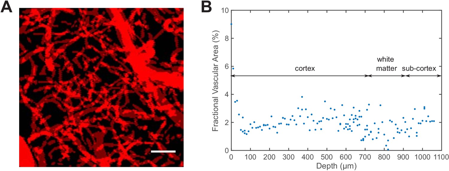
Measurement of the staining density in uniformly labeled vasculature.

(A) Z-projection of the identified blood vessels by summing all the XY-images in a vertical image stack (0–400 μm deep, with 10 μm step size). Scale bar, 30 μm. (B) The fractional vascular area in each XY-image at various depths.

Figure 2—figure supplement 1—source data 1 The area fraction of vasculature measured in the mouse brain, plotted in Figure 2—figure supplement 1.: https://cdn.elifesciences.org/articles/53205/elife-53205-fig2-figsupp1-data1-v2.csv
Download elife-53205-fig2-figsupp1-data1-v2.csv

Figure 2—figure supplement 2

Download asset Open asset

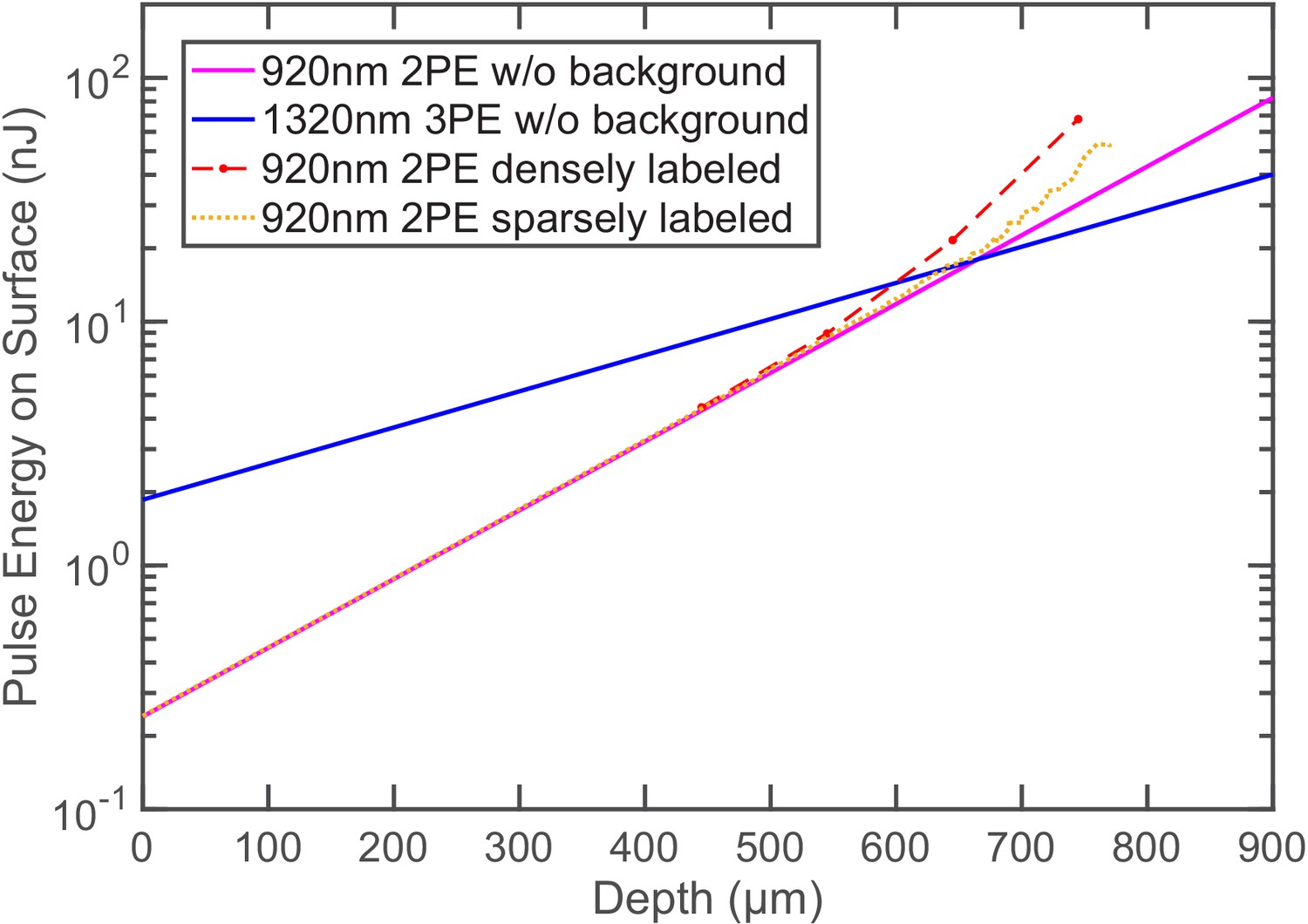
The pulse energy required at the brain surface to generate *the same* $d^{'}$ per pulse sampling the neuron for 2PE and 3PE of GCaMP6s at different imaging depths.

In the absence of the background fluorescence, $d^{'}$ is entirely determined by signal photon counts: when a neuron is sampled by 1000 excitation pulses in 1 s, it generates $F_{0} = 1000 p u l s e s \times 0.1 p h o t o n / p u l s e = 100 p h o t o n s / s$ , which gives $d^{'} \sim 3$ . Therefore, Group ‘920nm 2PE w/o background’ and ‘1320nm 3PE w/o background’ exactly reproduce the pulse energy curves for *the same signal* of 0.1 photon/excitation pulse (Figure 1B). Group ‘920nm 2PE densely labeled’ and ‘920nm 2PE sparsely labeled’ are calculated based on the SBR measured in GCaMP6s-labeled neurons and fluorescein-labeled blood vessels, respectively (Figure 2B). 1320-nm 3PE is assumed to be background-free in the mouse cortex.

Figure 3 with 5 supplements

Download asset Open asset

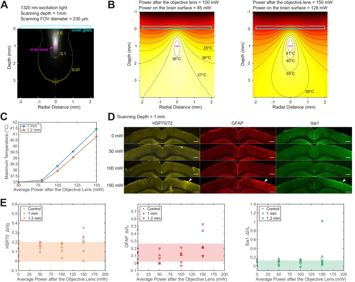
Brain heating and thermal damage induced by continuous scanning by 1320 nm 3PM.

(A) Monte Carlo simulation of light intensity of 1320 nm excitation light. The excitation light is focused at 1 mm below the brain surface in the cortex by an objective of 1.05 NA at ~75% filling of its back aperture and scanned telecentrically in a 230 μm diameter FOV (the horizontal magenta line segment). Three iso-contour lines (from inside to outside) correspond to 0.01, 0.1, and 0.5 of the maximum intensity. (B) Temperature maps under 1320 nm illumination calculated from the power absorption per unit volume in (A) after 60 s of continuous scanning with 100 and 150 mW average power after the objective lens. Temperature is color-coded with isotherms plotted at 1°C increment with the highest four temperature levels labeled. The average imaging power is listed at the top of each plot. (C) The maximum temperature versus imaging power for 1 mm and 1.2 mm focal depth, with other imaging parameters the same as in (A) and (B). The maximum temperature is calculated as the average in the hottest volume around the scanned area (~10⁷ μm³). (D) Immunolabeled brain slices of mouse brains after 1320 nm 3PM scanning with 0, 50 mW, 100 mW, and 150 mW average power (one mouse is shown for each power). The brain was scanned for 20 min continuously at 1 mm below the surface, with 230 μm x 230 μm FOV and 2 Hz frame rate. The location of the damage is indicated by the white arrowheads. Scale bar, 0.5 mm. (E) Quantification of heat-induced damage by the fractional change of immunolabeling intensity relative to the region in the contralateral hemisphere. Shaded areas denote 95% confidence interval of the control group mean (n = 4 mice for control; n = 6 mice for 50 mW; n = 5 mice for 100 mW; n = 7 mice for 150 mW).

Figure 3—source data 1 Quantification of the staining intensity of immunolabeld mouse brain slices post mortem after the exporsure to continuous 1320 nm 3PM scanning, plotted in Figure 3E.: https://cdn.elifesciences.org/articles/53205/elife-53205-fig3-data1-v2.zip
Download elife-53205-fig3-data1-v2.zip

Figure 3—figure supplement 1

Download asset Open asset

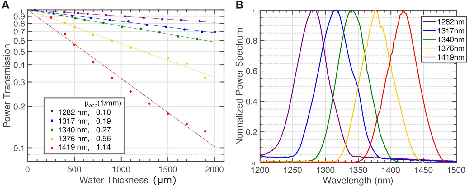
Light attenuation by immersion water for various excitation wavelengths.

(A) Power transmission versus immersion water thickness under the objective (Olympus XLPLN25XWMP2, 25X, NA=1.05, ~ 75% filling of the back aperture) for 5 spectra centered from 1280 nm to 1420 nm using broadband pulses from the NOPA. Each transmission curve is fitted with a single exponential function to calculate the apparent attenuation coefficient ( $μ_{a p p}$ ). The inset lists these coefficients. (B) The spectra of the pulses for the transmission measurement in (A).

Figure 3—figure supplement 1—source data 1 Power transmission through immersion water of different thicknesses under the objective lens, measured with different excitation spectra and plotted in Figure 3—figure supplement 1.: https://cdn.elifesciences.org/articles/53205/elife-53205-fig3-figsupp1-data1-v2.xlsx
Download elife-53205-fig3-figsupp1-data1-v2.xlsx

Figure 3—figure supplement 2

Download asset Open asset

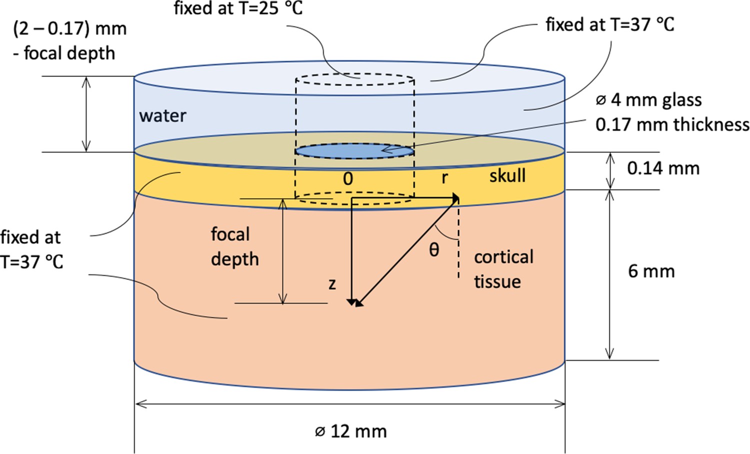
Spatial dimension, coordinate system, and boundary conditions for Monte Carlo and heat conduction simulation.

Figure 3—figure supplement 3

Download asset Open asset

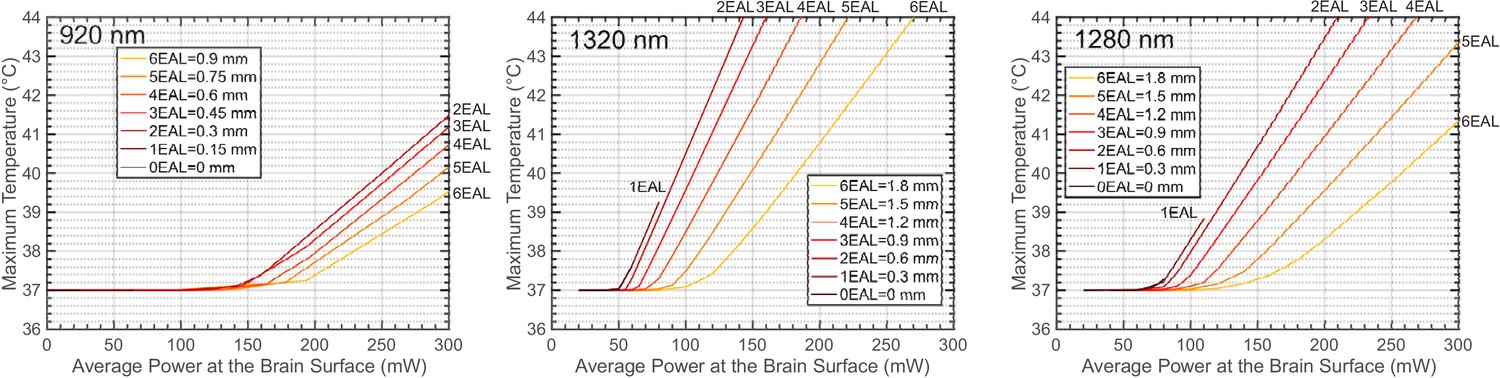
The maximum brain temperature as a function of the average power at the brain surface, shown for different imaging depths at 920 nm, 1320 nm, and 1280 nm.

The imaging depth grows in the increment of the nominal EAL of the cortex, which is 150 μm for 920 nm and 300 μm for both 1320 nm and 1280 nm. The linear scanning FOV diameter is 300 μm, and other parameters used for the simulation are listed in Table 1 and Table 3. For 1320 nm, the power immediately after the objective lens can be calculated by multiplying the power at the brain surface with a factor to correct for immersion water absorption: 1.42, 1.33, 1.27, 1.20, 1.13, 1.07, and 1.01 (from 0 to 6 EALs). For 1280 nm, the correction factors are: 1.20, 1.17, 1.13, 1.10, 1.07, 1.03, and 1.00 (from 0 to 6 EALs).

Figure 3—figure supplement 4

Download asset Open asset

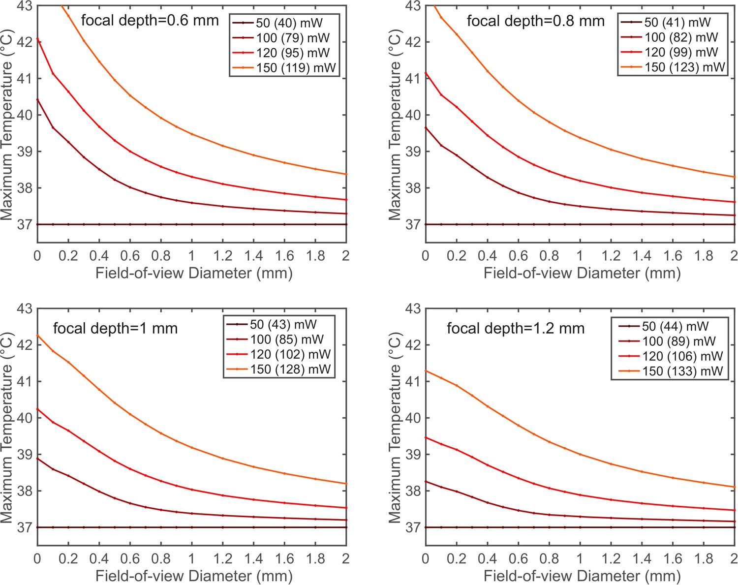
The maximum brain temperature decreases with the scanning field-of-view.

The simulation was performed for 1320 nm excitation wavelength at 1- and 1.2 mm imaging depth with various average powers after the objective lens. The NA and the back-aperture beam size remain the same as in Figure 3A. Each legend key indicates the power immediately after the objective lens, followed by the power at the brain surface after immersion water absorption (in the bracket).

Figure 3—figure supplement 5

Download asset Open asset

Immunostaining reveals brain tissue damage by 1320 nm 3PM with 150 mW imaging power after the objective lens at 1.2 mm imaging depth.

The scanning was performed with 230 μm FOV for 20 min at various average powers in the mouse brain. The window and scanning area are on the right side of each brain slice, and the location of heating is indicated with white arrowheads. Scale bar, 500 μm.

Tables

Table 1

Optical parameters of gray matter.

Variable	Parameter	Wavelength	Value	Units
$μ_{a}$	absorption coefficient	920	0.039	1/mm
		1280	0.078	1/mm
		1320	0.12	1/mm
$μ_{s}$	scattering coefficient	920	6.7	1/mm
		1280	3.2	1/mm
		1320	3.2	1/mm
$g$	anisotropy coefficient	All	0.9	dimensionless
$n$	refractive index	All	1.36	dimensionless

Table 2

Percentage of Excitation Photons for Various Final Destinations.

	920 nm	1320 nm	1280 nm
Contributing to heating	20	63	49
Back scattered to window	25	9	10
Back scattered to skull	20	9	11
Escaped*	35	19	30

^*Photons escape the simulation volume by traveling too far (>6 mm) from the center of the cranial window or too deep (>6 mm) from the tissue surface.

Key resources table

Reagent type (species) or resource	Designation	Source or reference	Identifiers	Additional information
Strain, strain background (Mus musculus)	B6.Cg-Tg(CamK2a-tTA)1Mmay/J	The Jackson Laborartory Stock: 007004	MGI:2179066
Strain, strain background (Mus musculus)	B6;DBA-Tg(tetO-GCaMP6s)2Niell/J	The Jackson Laborartory Stock: 024742	MGI:5553332
Antibody	anti-HSP70/72 (mouse monoclonal)	Enzo Life Sciences, Cat# SPA-810PED	RRID:AB-2264369	IHC(1:400)
Antibody	anti-GFAP (mouse monoclonal)	Sigma-Aldrich, Cat# G3893	RRID:AB_477010	IHC(1:760)
Antibody	anti-Iba1 (mouse monoclonal)	Sigma-Aldrich, Cat# SAB2702364	RRID:AB_2820253	IHC(1:1000)
Antibody	Goat anti-mouse (polyclonal)	Thermo Fisher Scientific, Cat# A-11003	RRID:AB_2534071	IHC(1:500)
Software, algorithm	Source code 1: matlab code for simulating the brain temperature distribution under continuous long-wavelength illumination by 3PM using Monte Carlo method and heat equation.	Mathworks, Matlab 2016b	RRID:SCR_001622

Table 3

Thermal and mechanical properties of gray matter (Stujenske et al., 2015).

Variable	Parameter	Value	Units
$ρ$	Density	1.04 × 10⁻³	g/mm³
$c$	Brain specific heat	3.65 × 10³	mJ/g°C
$k$	Thermal conductivity	0.527	mW/mm °C
$ρ_{b}$	Blood density	1.06 × 10⁻³	g/mm³
$c_{b}$	Blood specific heat	3.6 × 10³	mJ/g°C
$w_{b}$	Blood perfusion rate	8.5 × 10⁻³	/s
$q$	Metabolic heat	9.5 × 10⁻³	mW/mm³
$T_{A}$	Arterial temperature	36.7	°C

Appendix 1—table 1

Two- and three-photon excitation parameters.

	Objective lens focal length (mm)	1/e²beam diameter at the back aperture (mm)	Effective NA	Pulse duration $τ$ (fs)	$g_{p}^{(n)}$
920 nm 2PE	7.2	11	0.75	60	0.66
1320 nm 3PE	7.2	11	0.75	60	0.51

Additional files

Source code 1 Matlab code for simulating the brain temperature distribution under continuous long-wavelength illumination by 3PM using Monte Carlo method and heat equation, which was used to produce Figure 3B and C, Figure 3—figure supplements 3 and 4.: https://cdn.elifesciences.org/articles/53205/elife-53205-code1-v2.zip
Download elife-53205-code1-v2.zip
Transparent reporting form: https://cdn.elifesciences.org/articles/53205/elife-53205-transrepform-v2.docx
Download elife-53205-transrepform-v2.docx

Download links

A two-part list of links to download the article, or parts of the article, in various formats.

Downloads (link to download the article as PDF)

Open citations (links to open the citations from this article in various online reference manager services)

Mendeley

Cite this article (links to download the citations from this article in formats compatible with various reference manager tools)

Tianyu Wang
Chunyan Wu
Dimitre G Ouzounov
Wenchao Gu
Fei Xia
Minsu Kim
Xusan Yang
Melissa R Warden
Chris Xu

(2020)

Quantitative analysis of 1300-nm three-photon calcium imaging in the mouse brain

eLife 9:e53205.

https://doi.org/10.7554/eLife.53205

Figures

Comparison of the power attenuation of 1320 nm and 920 nm excitation light and their respective 3-photon and 2-photon excitation efficiency in the mouse brain.

Figure 1—source data 1

Figure 1—source data 2

Figure 1—source data 3

Additional power attenuation curves of 920 nm and 1320 nm excitation light in the mouse neocortex (n = 3, >12 weeks old mice, all males).

Figure 1—figure supplement 1—source data 1

Comparison of signal-to-background ratio for 1320 nm 3PM and 920 nm 2PM in the non-sparsely labeled mouse brain and its effect on calcium imaging sensitivity.

Figure 2—source data 1

Figure 2—source data 2

Figure 2—source data 3

Figure 2—source data 4

Figure 2—source data 5

Measurement of the staining density in uniformly labeled vasculature.

Figure 2—figure supplement 1—source data 1

The pulse energy required at the brain surface to generate the same $d^{'}$ per pulse sampling the neuron for 2PE and 3PE of GCaMP6s at different imaging depths.

Brain heating and thermal damage induced by continuous scanning by 1320 nm 3PM.

Figure 3—source data 1

Light attenuation by immersion water for various excitation wavelengths.

Figure 3—figure supplement 1—source data 1

Spatial dimension, coordinate system, and boundary conditions for Monte Carlo and heat conduction simulation.

The maximum brain temperature as a function of the average power at the brain surface, shown for different imaging depths at 920 nm, 1320 nm, and 1280 nm.

The maximum brain temperature decreases with the scanning field-of-view.

Immunostaining reveals brain tissue damage by 1320 nm 3PM with 150 mW imaging power after the objective lens at 1.2 mm imaging depth.

Tables

Optical parameters of gray matter.

Percentage of Excitation Photons for Various Final Destinations.

Thermal and mechanical properties of gray matter (Stujenske et al., 2015).

Two- and three-photon excitation parameters.

Additional files

Source code 1

Transparent reporting form

Download links

Downloads (link to download the article as PDF)

Open citations (links to open the citations from this article in various online reference manager services)

Cite this article (links to download the citations from this article in formats compatible with various reference manager tools)

Be the first to read new articles from eLife

Share this article

Cite this article

Comparison of the power attenuation of 1320 nm and 920 nm excitation light and their respective 3-photon and 2-photon excitation efficiency in the mouse brain.

Figure 1—source data 1

Figure 1—source data 2

Figure 1—source data 3

Additional power attenuation curves of 920 nm and 1320 nm excitation light in the mouse neocortex (n = 3, >12 weeks old mice, all males).

Figure 1—figure supplement 1—source data 1

Comparison of signal-to-background ratio for 1320 nm 3PM and 920 nm 2PM in the non-sparsely labeled mouse brain and its effect on calcium imaging sensitivity.

Figure 2—source data 1

Figure 2—source data 2

Figure 2—source data 3

Figure 2—source data 4

Figure 2—source data 5

Measurement of the staining density in uniformly labeled vasculature.

Figure 2—figure supplement 1—source data 1

The pulse energy required at the brain surface to generate the same d′ per pulse sampling the neuron for 2PE and 3PE of GCaMP6s at different imaging depths.

Brain heating and thermal damage induced by continuous scanning by 1320 nm 3PM.

Figure 3—source data 1

Light attenuation by immersion water for various excitation wavelengths.

Figure 3—figure supplement 1—source data 1

Spatial dimension, coordinate system, and boundary conditions for Monte Carlo and heat conduction simulation.

The maximum brain temperature as a function of the average power at the brain surface, shown for different imaging depths at 920 nm, 1320 nm, and 1280 nm.

The maximum brain temperature decreases with the scanning field-of-view.

Immunostaining reveals brain tissue damage by 1320 nm 3PM with 150 mW imaging power after the objective lens at 1.2 mm imaging depth.

Optical parameters of gray matter.

Percentage of Excitation Photons for Various Final Destinations.

Thermal and mechanical properties of gray matter (Stujenske et al., 2015).

Two- and three-photon excitation parameters.

Source code 1

Transparent reporting form

Downloads (link to download the article as PDF)

Open citations (links to open the citations from this article in various online reference manager services)

Cite this article (links to download the citations from this article in formats compatible with various reference manager tools)

The pulse energy required at the brain surface to generate the same $d^{'}$ per pulse sampling the neuron for 2PE and 3PE of GCaMP6s at different imaging depths.