Cortical state transitions and stimulus response evolve along stiff and sloppy parameter dimensions, respectively
- Center for Brain and Cognition, Computational Neuroscience Group, Department of Information and Communication Technologies, Universitat Pompeu Fabra, Spain
- Institut d’Investigacions Biomèdiques August Pi i Sunyer (IDIBAPS), Spain
- Institució Catalana de la Recerca i Estudis Avançats (ICREA), Spain
- Department of Neuropsychology, Max Planck Institute for Human Cognitive and Brain Sciences, Germany
- School of Psychological Sciences, Monash University, Australia
Figures
Figure 1

Experiment and analysis designs.
(A) Each recording session was divided into adjacent epochs of 100 s. (B) Each epoch contained a series of stimulus presentations. Stimuli consisted on acoustic clicks. For each 100-s epoch we collected the spontaneous activity, that is the activity during 1.5-s intervals preceding each stimulus (red intervals), to build concatenated binary data. (C) Binary data was obtained by discretizing time in bins of dt = 10 ms. Within each time bin, the ensemble activity of neurons was described by a binary vector, , where if the i-th neuron generated a spike (black) and otherwise (white). (D) Maximum entropy models were used to describe the binary patterns of subsets of 10 neurons, during each 100-s epoch. The model parameters represents the intrinsic tendency of neuron i towards activation () or silence (), noted , and the effective interaction between neurons i and j, noted .
Figure 2
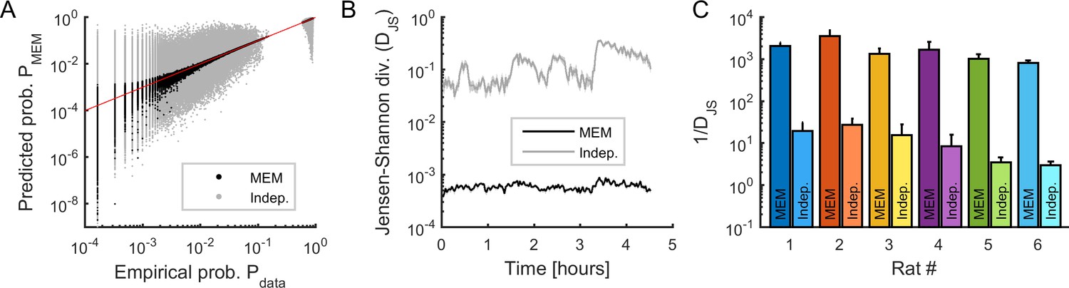
Fitting maximum entropy models (MEMs) to spontaneous activity patterns.
(A) Comparison between the probability distribution of empirical binary patterns and the probability distribution predicted by MEMs (black dots) and independent models (gray dots), for all epochs and all neuronal ensembles. Every point represents a binary pattern that has appeared in the data at least once. Red line represents the identity line. (B) Jensen-Shannon divergence (DJS) between spiking data and MEMs, and between spiking data and independent models, across time, averaged across neuronal ensembles. Error bars are smaller than the widths of the traces. Data in (A) and (B) correspond to one example rat (#1). (C) Goodness-of-fit (1/DJS) for MEMs and for independent models, averaged over all models (i.e., all ensembles and all epochs), for each rat. Error bars indicate SEM.
Figure 3
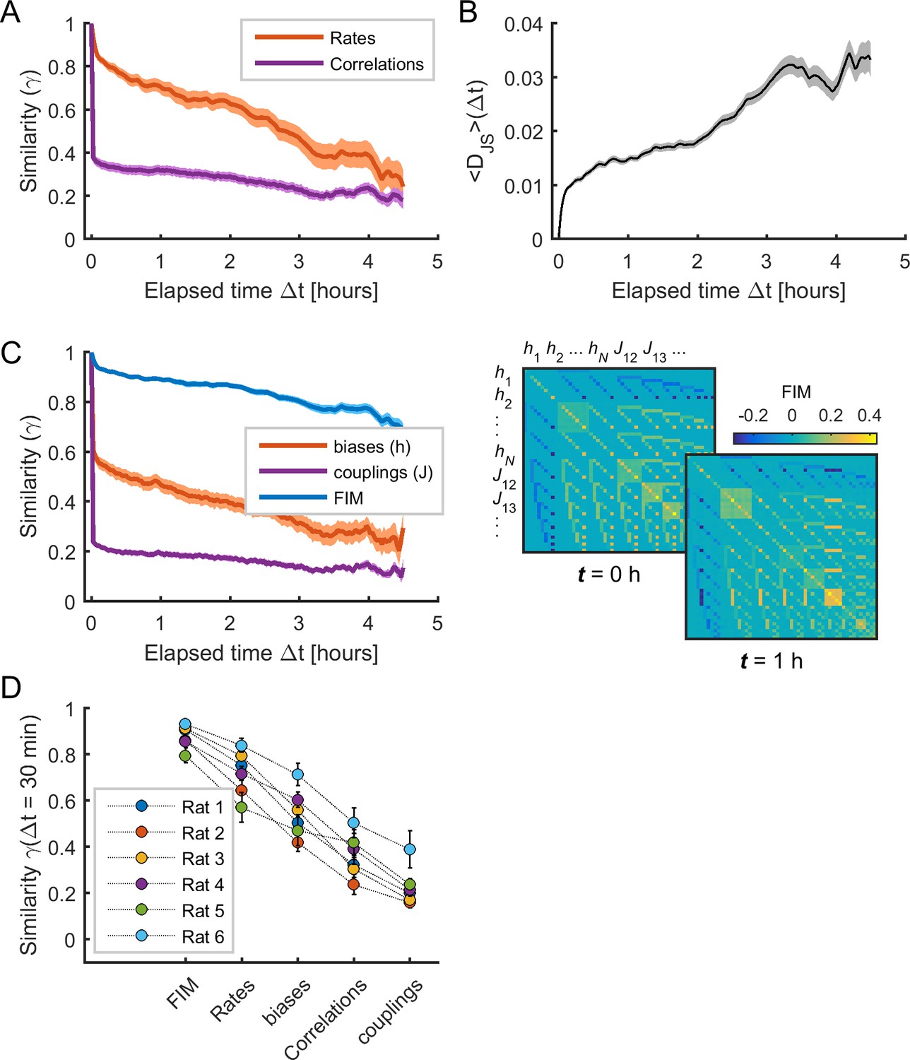
The sensitivity of model parameters was more stable than activity observables.
(A) Similarity (i.e., Pearson correlation coefficient) of mean firing rates (red) and pairwise correlations (purple) as a function of elapsed time Δt. (B) Jensen-Shannon divergence (DJS) between the distribution of empirical spiking patterns in epoch t and the distribution of binary patterns of the pairwise MEM in epoch t + Δt, averaged over all t. (C) Left: Similarity of Fisher information matrix (FIM) elements, biases (), and couplings () as a function of elapsed time Δt. Right: FIMs at time t = 0 h and t = 1 h. Data in (A), (B), and (C) correspond to one example rat (#1); traces show averages over neuronal ensembles and shaded areas correspond to SEM. (D) Similarity of FIM elements, rates, biases, correlations, and couplings after 1/2 hour (i.e., Δt = 30 min), averaged across all neuronal ensembles, for each rat. Error bars indicate SEM.
Figure 4 with 1 supplement
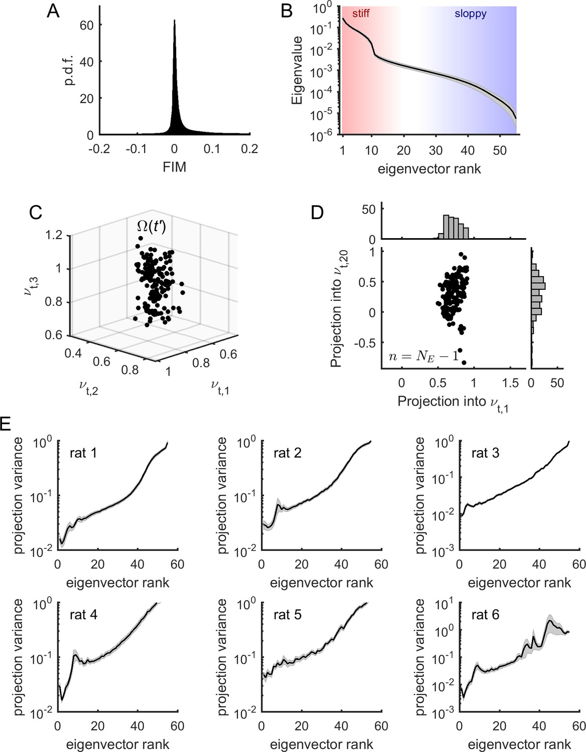
Model parameters presented sloppiness and predominantly evolved along sloppy dimensions.
(A) Distribution of FIM elements, for all epochs, all neuronal ensembles, and all rats. (B) Eigenvalues of the FIM, average across epochs and neuronal ensembles, for an example rat (# 1). Shaded areas represent SEM. Stiff and sloppy dimensions correspond to FIM eigenvectors of lowest and highest ranks, respectively. (C) Projection of into the first three eigenvectors of the FIM from a given epoch , for all . Data from one neuronal ensemble from rat 1. (D) Projection of into the first and the 20th eigenvectors of the FIM from epoch , noted and , respectively, for all . Top inset: distribution of projections into . Right inset: distribution of projections into . Note higher variance of projections into than into . Data from one neuronal ensemble from rat 1. (E) Average variance of projections of into the different eigenvectors of the FIM at epoch (for all ), for the different rats. Traces represent average over neuronal ensembles and shaded areas represent SEM.
Figure 4—figure supplement 1
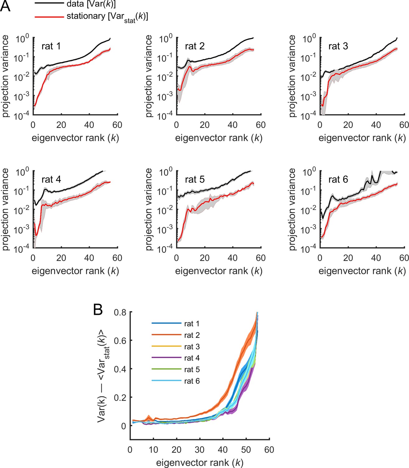
Parameters projections into FIM eigenvectors: data vs. stationary surrogates.
The variance of projections of into the different eigenvectors of the Fisher information matrix (FIM) for spiking data was compared to the one obtained from stationary surrogates. (A) The average variance of projections of model parameters into the different eigenvectors of the FIMs was calculated for the spiking data (parameters ) and for the stationary surrogates (parameters ), as a function of the rank of the eigenvectors. Variances were noted and for the spiking data and the stationary surrogates, respectively. Traces represent average over neuronal ensembles and shaded areas represent SEM. Note logarithmic scale on the y-axis. We found that parameter fluctuations were larger than expected by estimation errors in the stationary case for all eigenvectors (i.e., , for all ). (B) The difference between variances of parameter projections estimated from the spiking data and those estimated from stationary surrogates increased with . Thus, parameter fluctuations along sloppy dimensions were those that deviated the most from the stationary case. Traces represent average over neuronal ensembles and shaded areas represent SEM.
Figure 5 with 1 supplement

Spontaneous neuronal activity evolved along stiff dimensions during cortical state transitions.
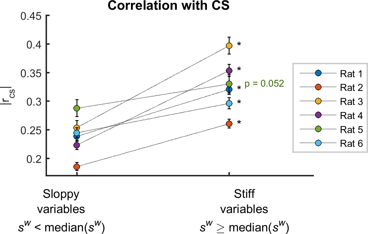
(A) Silence density was used to characterize the cortical state. Green inset: low values of the silence density indicate desynchronized cortical states (each row represents the spike train of a single-unit). Red inset: high values of the silence density indicate synchronized cortical states. Data from rat 1. (B) Difference in collective pattern statistics, that is DJS, between different epochs, and , as a function of the corresponding difference in silence density, noted d. Each gray dot corresponds to a pair of epochs (). The solid line indicates the average relation between DJS and d; error bars indicate SD. Data from all neuronal ensembles from rat 1. (C) Correlation coefficient between DJS and d, for all rats. *: p < 0.001. (D) Top: Distribution of the absolute value of the correlations between the cortical state and the activity observables, noted . Bottom: Distribution of parameter sensitivity values for biases (h parameters) and couplings (J parameters), for all models from all rats. (E) vs. sensitivity of all activity variables (i.e., firing rates and pairwise correlations). Correlation: = 0.36; p <0.001. Data from rat 4 ( = 72). (F) Correlation between and the sensitivity for each dataset. *: p < 0.001. Error bars indicate correlation 95% confidence interval. (G) for sloppy and stiff variables. *: p < 0.001, paired t-test. Error bars indicate SEM.
Figure 5—figure supplement 1
Alternative definition of sensitivity.
Averaged correlation between observables and cortical state, , for sloppy and stiff variables, for weighted sensitivity defined using equation 9. *: p < 0.001, paired t-test. Error bars indicate SEM.
Figure 6 with 1 supplement
Stimulus-evoked neuronal activity evolved along sloppy dimensions.
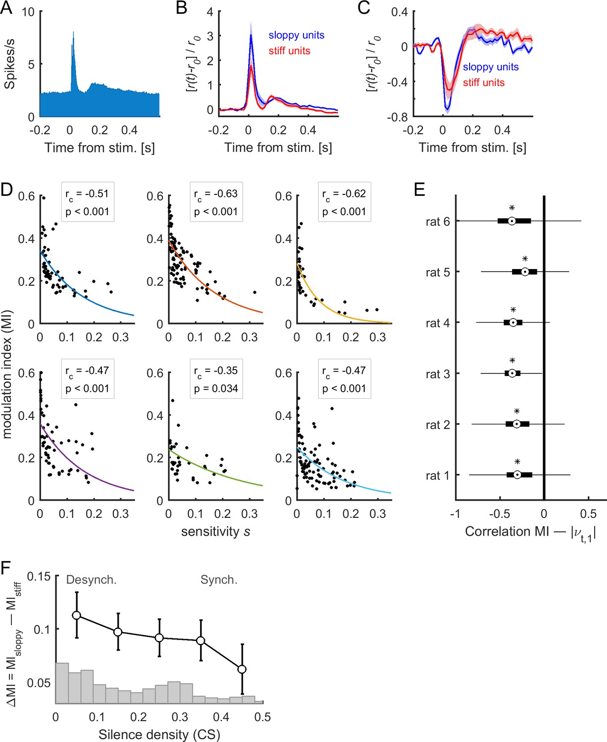
(A) Population responses to acoustic clicks. (B–C) Median-split of sensitivity was used to separate stiff neurons and sloppy neurons. The mean responses for stiff and sloppy neurons are shown in the case of excited responses (B) and suppressed responses (C). The responses were normalized by the average pre-stimulus activity . Shaded areas correspond to SEM. Data in (A), (B), and (C) correspond to one example rat (#1). (D) Modulation index (MI) as a function of associated sensitivity of firing rates (, with 1 ), for each dataset. Each dot corresponds to a single neuron of the recorded population. The correlation between MI and sensitivity was negative for all datasets (: correlation coefficient; p: p-value). Solid lines indicate exponential fits. (E) Correlation between MI(t), calculated in epoch , and , for all neuronal ensembles of each of the rats. On each box, the central mark indicates the median, and the bottom and top edges of the box indicate the 25th and 75th percentiles, respectively. Asterisks indicate significantly negative medians (p < 0.001, two-sided signed rank test). (F) Difference of the MI of sloppy neurons minus the MI of stiff neurons as a function of cortical state (i.e., silence density), averaged for all rats (black trace; error bars indicate SEM). The gray bars indicate the distribution of silence density values.
Figure 6—figure supplement 1
Alternative definition of sensitivity.
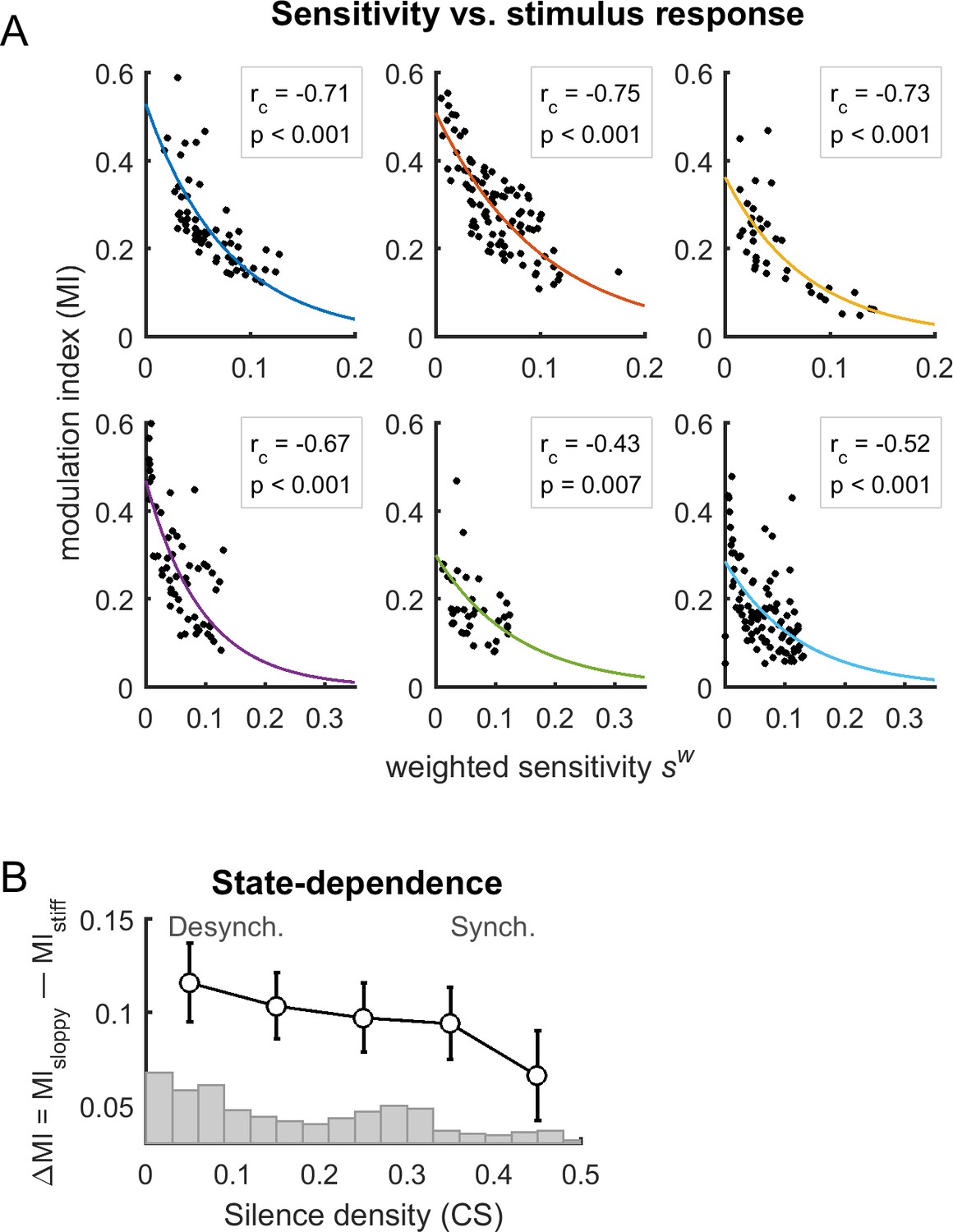
(A) Modulation index (MI) as a function of associated weighted sensitivity of firing rates, for each dataset. The correlation between MI and was negative for all datasets (: correlation coefficient; p: p-value). Solid lines indicate exponential fits. (B) Difference of the MI of sloppy neurons minus the MI of stiff neurons as a function of cortical state (i.e., silence density), averaged for all rats (black trace; error bars indicate SEM). The gray bars indicate the distribution of silence density values.
Figure 7 with 1 supplement

Central and highly active neurons were associated to stiff parameters.
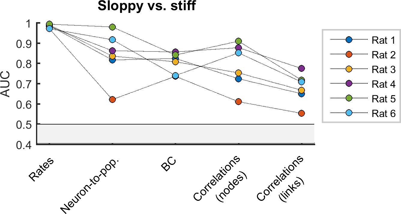
(A) Distribution of firing rates of sloppy and stiff neurons. (B) Distribution of correlations among sloppy neurons and among stiff neurons. (C) The distribution of correlations was also calculated for the links (i.e, pairs of neurons with associated parameters ). Note that, in principle, links can be related to pairs composed of one sloppy and one stiff neuron. (D) Distribution of betweenness centrality of sloppy and stiff neurons. (E) Connectivity graph: each node represents a neuron and links represent significant correlations between pairs of neurons. The graph was plotted using force-directed layout, that is using attractive forces between strongly connected nodes and repulsive forces between weakly connected nodes. Left: the nodes were colored as a function of betweenness centrality. Right: the nodes were colored as a function of associated sensitivity . Note the high overlap between both color labeling methods, indicating that sensitivity was highly predictive of the centrality of the nodes. (F) Distribution of neuron-to-population couplings of sloppy and stiff units. Panels A–F show data from rat 1. (G) Area under the receiver operating curve (AUC) quantifying the separation of distributions of sloppy and stiff classes. All AUC values were significantly higher than 0.5 (p < 0.001).
Figure 7—figure supplement 1
Alternative definition of sensitivity.
Area under the receiver operating curve (AUC) quantifying the separation of distributions of sloppy and stiff classes using the weighted sensitivity defined using equation 9. All AUC values were significantly higher than 0.5 (p < 0.001).
Appendix 1—figure 1
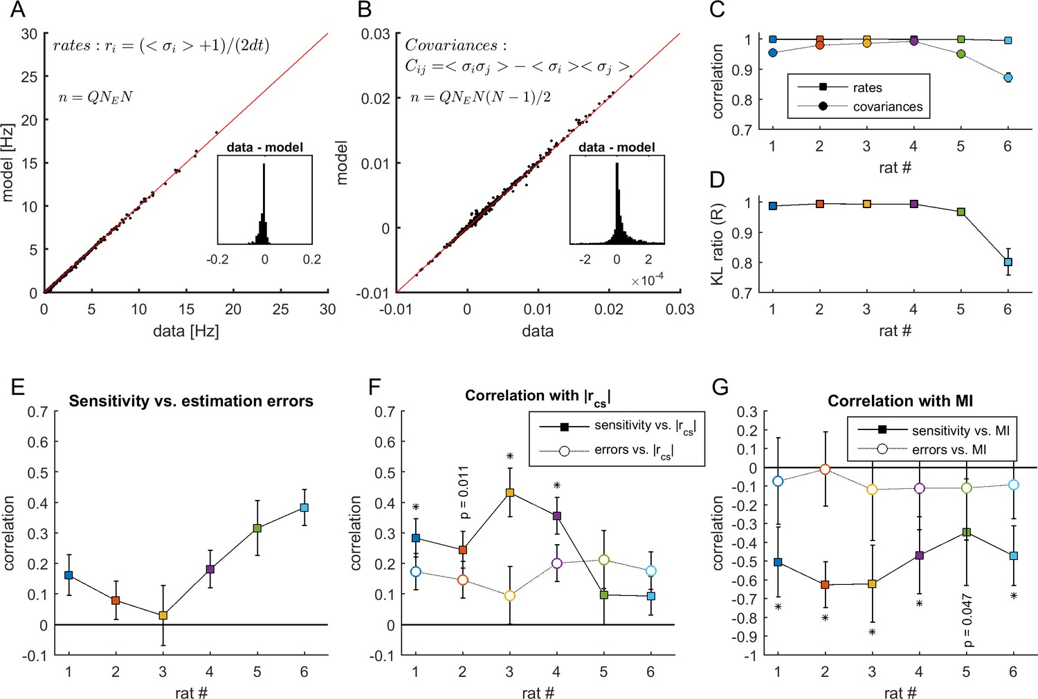
Estimation errors and sensitivity.
(A-B) Comparison between the firing rates and covariances measured in the data and those estimated by the MEM. Data from rat 4. Each point represents the activity of a neuron (in panel A) or co-activity of a pair of neurons (in panel B) from a given neuronal ensemble and at a given epoch. The data of all neuronal ensembles and all epochs are presented. Insets show the resulting differences between statistics estimated from the data and from the model. (C) Correlation between the firing rates and covariances measured in the data and those estimated by the MEM, for each dataset. (D) Average Kullback-Leibler ratios for all learned models of each dataset. Error bars indicate SEM. (E) Correlation between sensitivity and estimation errors . (F) Full squares: correlation between sensitivity and (same values as in Figure 5F). Open circles: correlation between estimation errors and . For each dataset the correlation coefficients were compared, given the observed correlations in panel E using Meng's z-test for dependent correlations, *: p < 0.01. (G) Full squares: correlation between sensitivity of firing rates and MI (same values as in Figure 6D). Open circles: correlation between firing rate estimation errors and MI. *: p < 0.01, Meng's z-test for dependent correlations. In panels (C) and (E–G), error bars indicate correlation 95% confidence interval.
Appendix 1—figure 2
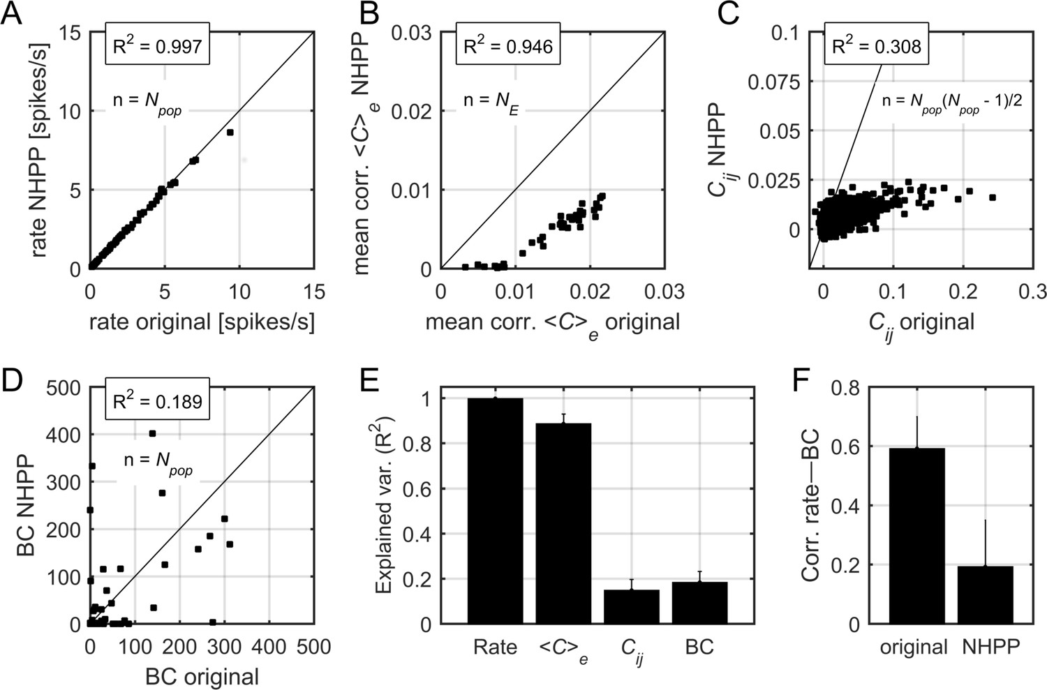
Correlations and centrality in non-homogeneous Poisson process surrogate data.
(A) Relation between firing rates in the original data and firing rates in the non-homogeneous Poisson process (NHPP) surrogates. R2 indicates the fraction of explained variance. The black line indicates the identity line. (B) Relation between the mean pairwise correlation in the original data and that in NHPP surrogates. Each point represents the mean correlation (averaged over neurons) in a given epoch. (C) Relation between pairwise correlations, averaged over the epochs, in the original data and those in NHPP surrogates. Each point represents a pair of neurons. (D) Relation between BC values in the original data and those in NHPP surrogates (see Materials and methods for calculation of BC). Data in (A), (B), (C), and (D) correspond to one example rat. (E) Explained variance for firing rates, correlations, and BC values, averaged over datasets. Error bars indicate SEM. (F) Correlation between firing rates and BC values, averaged over datasets. Error bars indicate SEM.
Author response image 1

Tables
Key resources table
| Reagent type (species) or resource | Designation | Source or reference | Identifiers | Additional information |
|---|---|---|---|---|
| Biological sample (Sprague–Dawley rat) | Sprague–Dawley rat | https://doi.org/10.1073/pnas.1410509112 | six rats, 250–400 g | |
| Software, algorithm | Matlab | MathWorks | RRID:SCR_001622 | All analyses |
| Software, algorithm | Klustakwik | http://klustakwik.sourceforge.net/ | RRID:SCR_014480 | Spike sorting (detection and initial clustering) |
| Software, algorithm | EToS | http://etos.sourceforge.net/ | Spike sorting (detection and initial clustering) | |
| Software, algorithm | Klusters | http://neurosuite.sourceforge.net/ | Spike sorting (clustering) |
Table 1
Number of neurons (SU: single-units, MU: multi-unit), number of 100 s epochs, number of stimulus presentations in 100 s epochs, and number of neuronal ensembles, for each dataset.
| No. of neurons | No. of 100 s epochs | Stimulus presentations in 100 s epochs | No. of neuronal ensembles (Q) | |
|---|---|---|---|---|
| Rat 1 | SU: 81; MU: 3 | 163 | 12–14 | 20 |
| Rat 2 | SU: 147; MU: 13 | 74 | 12–14 | 20 |
| Rat 3 | SU: 44; MU: 30 | 70 | 12–20 | 10 |
| Rat 4 | SU: 72; MU: 103 | 59 | 10–20 | 20 |
| Rat 5 | SU: 58; MU: 39 | 29 | 28–29 | 10 |
| Rat 6 | SU: 112; MU: 83 | 28 | 17–29 | 20 |
Additional files
Download links
A two-part list of links to download the article, or parts of the article, in various formats.
Downloads (link to download the article as PDF)
Open citations (links to open the citations from this article in various online reference manager services)
Cite this article (links to download the citations from this article in formats compatible with various reference manager tools)
Cortical state transitions and stimulus response evolve along stiff and sloppy parameter dimensions, respectively
eLife 9:e53268.
https://doi.org/10.7554/eLife.53268


