Research Article

Eco-evolutionary dynamics of nested Darwinian populations and the emergence of community-level heredity

Laboratoire de Génétique de l'Evolution, Chimie Biologie et Innovation, Université PSL, France
Institut de Biologie de l’École Normale Supérieure (IBENS), École Normale Supérieure, Université PSL, France
Laboratoire de Probabilités, Statistique et Modélisation (LPSM), Sorbonne Université, CNRS, France
Center for Interdisciplinary Research in Biology (CIRB), Collège de France, Université PSL, CNRS, INSERM, France
Department of Evolutionary Theory, Max Planck Institute for Evolutionary Biology, Germany
Department of Microbial Population Biology, Max Planck Institute for Evolutionary Biology, Germany

Jul 7, 2020

https://doi.org/10.7554/eLife.53433

Open access
Copyright information

Figures
Additional files

22 figures and 2 additional files

Figures

Figure 1

Download asset Open asset

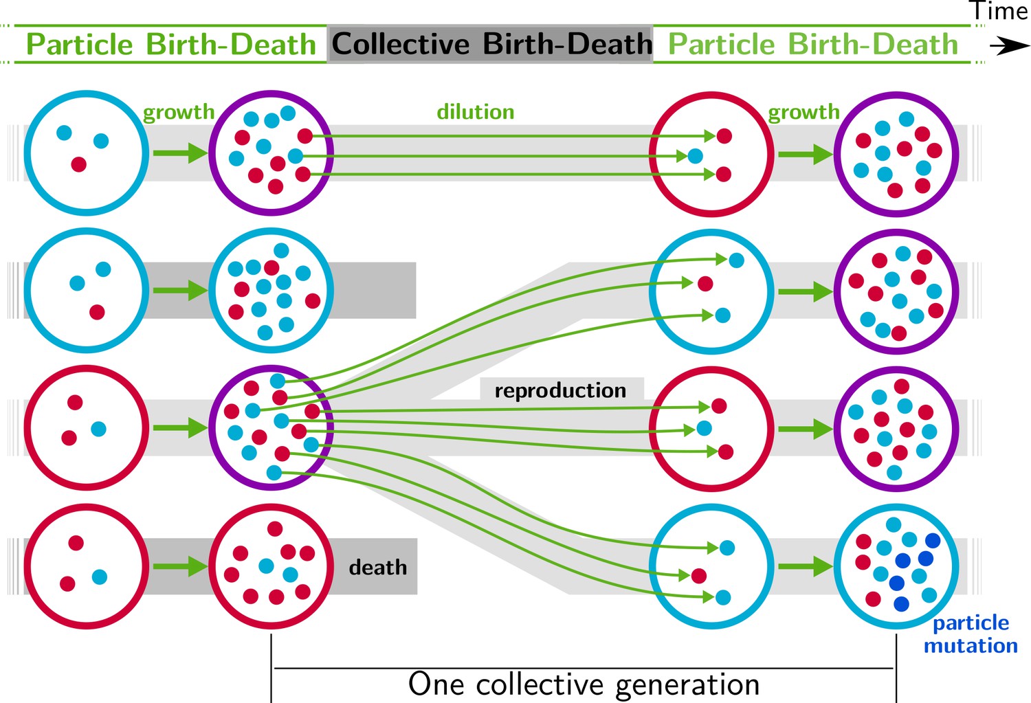
Nested model of evolution.

Collectives (large circles) follow a birth-death process (grey) with non-overlapping generations. Collectives are composed of particles (small spheres) that also follow a birth-death process (growth, represented by thick green arrows). Offspring collectives are founded by sampling particles from parent collectives (dilution, represented by thin green arrows, first and third rows). Survival of collectives depends on colour. Collectives that contain too many blue (second row) or red (fourth row) particles are marked for extinction. The number of collectives is kept constant. Mutation affects particle traits (see main text for details).

Figure 2

Download asset Open asset

Evolutionary dynamics of collectives and particles.

A population of $D$ = 1000 D collectives was allowed to evolve for $M$ = 10,000 generations under the stochastic birth-death model described in the main text (see Appendix 1 for details on the algorithm used for the numerical simulations). Initially, each collective was composed of $B = 15$ particles of two types: red ( $r_{0} = 6, a_{0}^{intra} = 0.8 / K, a_{0}^{inter} = 0.15 / K, c_{0} = red$ ) and blue ( $r_{1} = 4, a_{1}^{intra} = 0.3 / K, a_{1}^{inter} = 0.15 / K, c_{1} = blue$ ), with $K$ = 1500. The proportions at generation 0 were randomly drawn from a uniform distribution. At the beginning of every successive collective generation, each offspring collective was seeded with founding particles sampled from its parent. Particles were then grown for a duration of $T$ = 1. When the adult stage was attained, 200 collectives ( $ρ = 20 %$ ) were extinguished, allowing opportunity for extant collectives to reproduce. Collectives were marked for extinction either uniformly at random (neutral regime, panels A, C, E, as well as Appendix 1—figures 1A and 4A), or based on departure of the adult colour from the optimal purple colour ( $\hat{ϕ} = 0.5$ ) (selective regime, panels B, D, F, as well as Appendix 1—figures 1B and 4B). Panels A and B, respectively, show how the distribution of the collective phenotype changes in the absence and presence of selection on collective colour. The first 30 collective generations (before the grey line) are magnified in order to make apparent early rapid changes. In the absence of collective-level selection purple collectives are lost in fewer than 10 generations leaving only red collectives (A) whereas purple collectives are maintained in the selective regime (B). Panels C-F illustrate time-resolved variation in the distribution of underlying particle traits. A diversity of traits is maintained in the population because every lineage harbours two sets of traits for every colour (see Appendix 1). Selection for purple-coloured collectives drives evolutionary increase in particle growth rate (D) compared to the neutral regime (C). In the neutral regime, inter-colour evolution of competition traits is driven by drift (E), whereas with collective-level selection density-dependent interaction rates between particles of different colours rapidly achieve evolutionarily stable values, with one colour loosing its density-dependence on the other (F).

Figure 3

Download asset Open asset

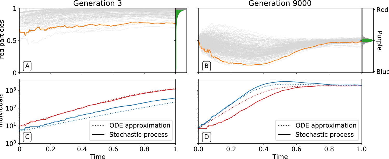
Ecological dynamics of particles.

A sample of 300 (from a total of 1000) collectives were taken from each of generations 3 (A,C) and 9000 (B,D) in the evolutionary trajectory of Figure 2. The dynamic of particles was simulated through a single collective generation ( $0 \leq t \leq T = 1$ ), based on the particle traits of each collective. Each grey line denotes a single collective. The frequency distribution of adult collective colour (the fraction of red particles at time $T$ ), is represented in the panel to the right. The grey area indicates the fraction $ρ$ of collectives whose adult colour is furthest from $\hat{ϕ} = 0.5$ , that will be eliminated in the following collective generation. Single orange lines indicate collectives whose growth dynamic — number of individual particles — is shown in C and D, respectively. Dotted lines show the deterministic approximation of the particle numbers during growth (Appendix 2 Equation 1). Initial trait values result in exponential growth of particles (C), leading to a systematic bias in collective colour towards fast growing types (A). Derived trait values after selection yield a saturating growth toward an equilibrium (B) leading to the re-establishment of the purple colour by the end of the generation, despite initial departure (A). This is associated to the transition from a skewed distribution of collective colour, where almost all collectives are equally bad, to a narrow distribution centered on the target colour.

Figure 4

Download asset Open asset

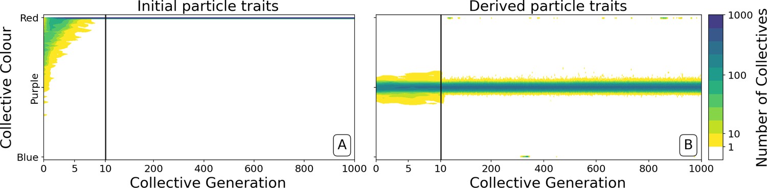
Dynamics of ancestral and derived collectives in the neutral regime.

Comparison of the dynamics of the colour distribution after removing selection (neutral regime). The population of 1000 collectives is initially composed of collectives with a colour distribution identical to that at generation 10,000 in Figure 2B. Particle traits are: (A) as in generation 1 of Figure 2; (B) derived after 10,000 generations of collective-level selection for purple. In both instances, particle mutation was turned off in order to focus on ecological dynamics, otherwise parameters are the same as in Figure 2A. Appendix 1—figure 6 shows the outcome with particle mutation turned on. The first 10 collective generations are magnified in order to make apparent the initial rapid changes. The particle traits derived after evolution are such that the majority of collectives maintains a composition close to the optimum $\hat{ϕ}$ even when the selective pressure is removed. This feature is instead rapidly lost in populations of collectives with the same initial colour, but with particle traits not tuned by evolution.

Figure 5

Download asset Open asset

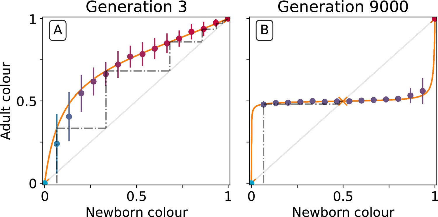
Effect of collective-level selection on newborn-to-adult colour.

The adult colour of collectives as a function of their newborn colour is displayed for collectives of uniformly distributed initial colour. Stochastic simulations are realized by using particle traits representative of: (A) generation 3 and (B) generation 9000 (as in Figure 3). Dots indicate the mean adult colour from 50 simulations and its standard deviation. The orange line depicts the growth function $G$ for the corresponding deterministic approximation (see main text and Appendix 2). The dashed line traces the discrete-time deterministic dynamics of the collective colour, starting from $ϕ = \frac{1}{B}$ , and across cycles of growth and noise-less dilution. For ancestral particle traits (A), collective colour converges towards the red monochromatic fixed point. After selection for collective colour (B), the growth function is such that the optimum colour ( $\hat{ϕ}$ ) is reliably produced within a single generation for virtually the whole range of possible founding colour ratios. The latter mechanism ensures efficient correction of alea occurring at birth and during development.

Figure 6

Download asset Open asset

Evolutionary variation of the growth function under collective selection.

function associated with the resident types for a single lineage of collectives from the simulation of Figure 2B, plotted every 20 collective generations from 0 to 9000. The result of iterations of $G$ gradually changes from fixation of the fast growing particle (Figure 5A) to convergence toward the colour purple (Figure 5B).

Figure 7

Download asset Open asset

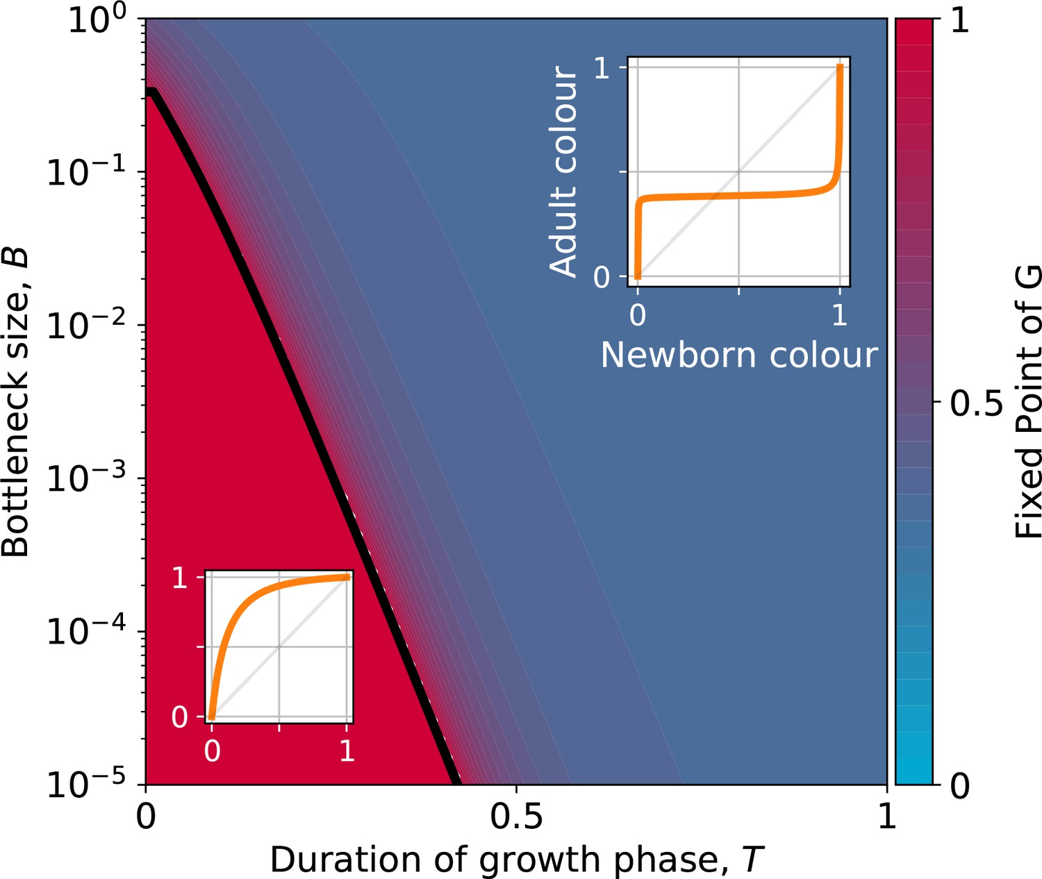
Stable fixed point of $G$ as a function of collective-level parameters.

Classification of the qualitative shape of the growth function and dependence on collective parameters B (bottleneck size) and T (growth phase duration). Considered here are particle traits that allow coexistence ( $a_{01} < a_{11}$ and $a_{10} < a_{00}$ , $r_{0} > r_{1}$ , see Appendix 2—figure 3 for the other possible parameter regions). The black line represents the limit of the region of stability of the fixed point of G, separating the two qualitatively different scenarios illustrated in the inset (see Appendix 2, Proposition 4 for its analytic derivation): for short collective generations and small bottleneck size, the faster growing red type competitively excludes the blue type over multiple collective generations. In order for particle types to coexist over the long term, growth rate and the initial number of particles must both be large enough for density-dependent effects to manifest at the time that selection is applied.

Figure 8

Download asset Open asset

Constrained evolutionary trajectories.

Dynamics through time of resident particle traits (black dots, whose size measures their abundance in the collective population) along simulated evolutionary trajectories of 300 generations, when particle-level traits are constrained. For both panels $D = 1000$ , $\hat{ϕ} = 0.5, ρ = 20 %$ , $B = 15$ , and $T = 1$ . The trajectory of the average resident traits is shown in white. The heatmap represents the value of $G (0.5)$ as a function of the evolvable traits, and the white dotted line indicates where collective colour is optimum. (A) Particle growth rates evolve and particles do not compete ( $a^{inter} = a^{i n t r a} = 0$ ). The evolutionary dynamics leads to alignment of growth rates ( $r_{0} = r_{1}$ ). (B) Inter-colour competition traits evolve and particle growth rates are constant ( $r_{0} = r_{1} = 25$ ). The evolutionary dynamics first converge toward the optimality line. In a second step, asymmetric competition evolves: $a_{1}^{inter} \to 0$ and $a_{0}^{inter} \to a_{0}^{intra} - a_{1}^{intra}$ . This results in a flatter $G$ function around the fixed point, providing a faster convergence to optimum colour across collective generations (Appendix 2—figure 6). Similar results are obtained for non-identical, but sufficiently high, growth rates.

Appendix 1—figure 1

Download asset Open asset

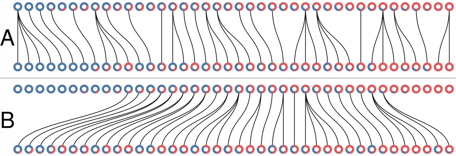
Collective-level selection regimes.

Each ring represents a collective. The blue section of the ring represents the proportion of blue particles at the adult stage of the collective. Parent and offspring are linked by a black line. (A) One generation of the neutral regime. (B) One generation of the selective regime. In both cases $M = 1, D = 40, ρ = 0.4$ .

Appendix 1—figure 2

Download asset Open asset

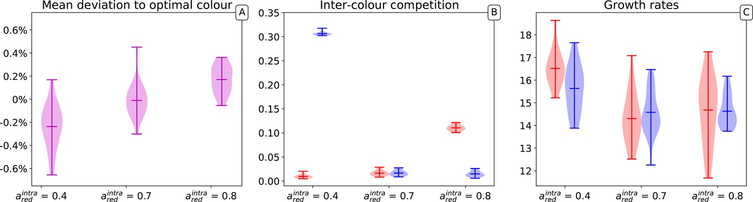
Distribution of average mutable traits values across several simulations.

Three parameters sets are represented in which red and blue types have respectively equal carrying capacity ( $a_{0}^{intra} = a_{1}^{intra} = 0.7 / K$ ), red types have a higher carrying capacity ( $a_{0}^{intra} = 0.4$ ) and lower carrying capacity ( $a_{0}^{intra} = 0.8$ ). The results of 20 independent simulations for each of the parameters sets are shown. For each simulation, $D = 100$ collectives, $M = 10, 000$ generations, $B = 15$ particles, the optimal collective colour is $\hat{ϕ} = 0.5$ and initial particle traits are $(r_{1} = r_{0} = 5, a_{1}^{intra} = 0.7 / K, a_{0}^{inter} = a_{1}^{inter} = 0.3 / K)$ , with $K = 1500$ .

Appendix 1—figure 3

Download asset Open asset

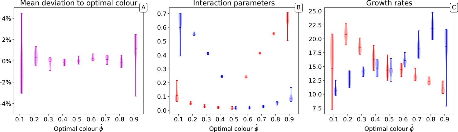
Distribution of the final traits across several experiments for different optimal colours.

Ten independent simulations are performed for each value of $\hat{ϕ}$ . In all simulations, $D = 100$ collectives, $M =$ 10,000 generations, $B = 15$ particles, and initial particle traits are $(r_{0} = r_{1} = 5, a_{0}^{intra} = a_{1}^{intra} = 0.7 / K, a_{0}^{inter} = a_{1}^{inter} = 0.3 / K)$ , with $K = 1500$ .

Appendix 1—figure 4

Download asset Open asset

Example of collective genealogy (Supplement of Figure 2).

Symbols and colours are as in Appendix 1—figure 1 and extinct lineages are marked transparent. Collective-level parameters in this simulation are $M = 30, D = 20, ρ = 0.1$ . A. Neutral regime: at the final generation, collectives are monochromatic and most likely composed of the faster-growing type. B. Selective regime: at the final generation, collectives contain both red and blue particles.

Appendix 1—figure 5

Download asset Open asset

The stochastic-corrector mechanism can maintain both types of particles in the absence of mutations (Supplement of Figure 2).

Collective phenotype distribution through time in the selective regime with ancestral particle traits and no mutations. Without collective-level mutation, the only mechanism maintaining both types within the population is the stochastic corrector, whereby a fraction of the collectives with colour closer to the target are propagated to the next collective generation. This means that at every generation the distribution of collective phenotypes is skewed towards the colour that has higher maximal growth rate, and the target colour is realized, in a small fraction of collective population, thanks to stochastic fluctuations in the composition at birth. Parameters are $D = 1000$ , $M = 1000$ , $\hat{ϕ} = 0.5$ , $B = 15$ and initial traits $(r_{0} = 6, a_{0}^{intra} = 0.8 / K, a_{0}^{inter} = 0.15 / K, c_{0} = red)$ for red particles and $(r_{1} = 4, a_{1}^{intra} = 0.3 / K, a_{1}^{inter} = 0.15 / K, c_{1} = blue)$ for blue particles, with $K = 1500$ . The initial proportions at generation 0 were randomly drawn from a uniform distribution.

Appendix 1—figure 6

Download asset Open asset

Particle trait mutations lead to slow loss of optimal collective colour after removal of collective-level selection (Supplement of Figure 4).

Modification of the collective phenotype distribution when particle traits mutate and no selection for colour is applied, starting from the particle traits after 10,000 generations of selection for purple colour (as in Figure 4B). Collectives continue to produce purple offspring for more than 200 generations, before drift of particle traits erodes developmental correction. In contrast, for the ancestral particle traits, lineages become monochromatic in less than 10 generations (Figure 4A).

Appendix 2—figure 1

Download asset Open asset

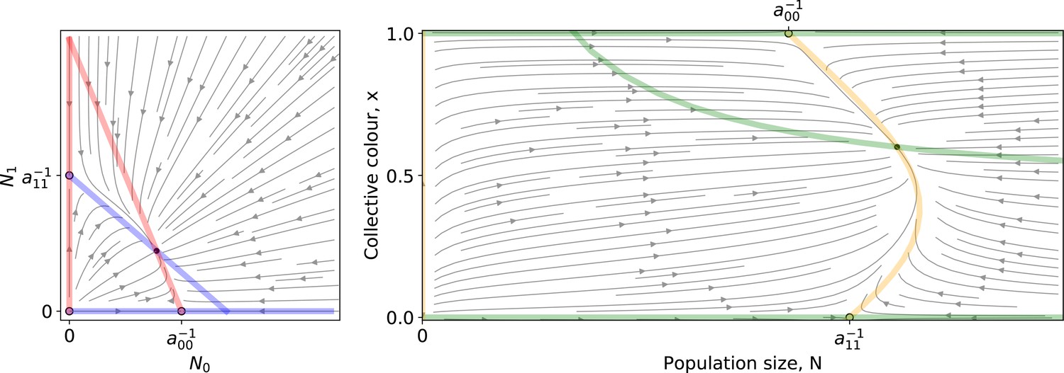
Left: A Lotka-Volterra flow (Equation 1 ) in $(N_{0}, N_{1})$ coordinates.

Right: The same flow in $(N, x)$ coordinates. Coloured lines are the null isoclines. Empty (resp. filled) circles mark unstable (resp. stable) equilibria.

Appendix 2—figure 2

Download asset Open asset

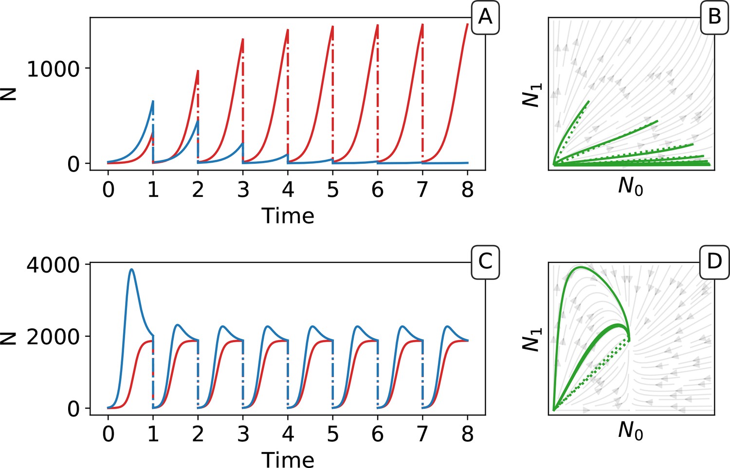
Piecewise continuous trajectory.

Iterating the deterministic model yields a piecewise continuous trajectory in the $(N_{0}, N_{1})$ space. The growth phase (continuous lines) alternates with the dilution (dotted lines). In (A, B) traits are taken from generation 3 and in (C,D) from generation 9000 of the main simulation with selection (Figure 2). Successive adult states can be computed using the $G_{θ}$ function as a recurrence map (see Figure 5 in the main text).

Appendix 2—figure 3

Download asset Open asset

Qualitative behaviours of the growth function $G_{θ}$ .

Panels 1–4 represent the possible qualitative shapes, differing in the position and stability of the fixed points, of the growth function $G_{θ}$ that approximates the within-collective particle dynamics (orange line in Figure 5). (1) $ϕ = 1$ is the only stable fixed point (Figure 5A), and iteration of the red $G_{θ}$ function leads to fixation of red particles. (2) $ϕ = 0$ is the only stable fixed point, and iteration of the blue $G_{θ}$ function leads to fixation of blue particles. (3) $ϕ = 0$ and $ϕ = 1$ are two stable fixed points, and iteration of the grey $G_{θ}$ function leads to fixation of either red or blue particles depending on initial conditions. (4) $ϕ = 0$ and $ϕ = 1$ are unstable and there is a stable fixed point between 0 and 1. Iteration of the grey $G_{θ}$ function leads to coexistence of both particle types. Panels (A-D) show that when red particles are the fast growing types ( $r_{0} > r_{1}$ ), the shape of $G_{θ}$ and the position of its fixed points depend on the collective-level parameters $B$ (bottleneck size) and $T$ (growth phase duration). Particle interaction traits generically belong to one of the four intervals (A) $a_{01} < a_{11}$ and $a_{00} < a_{10}$ ; (B) $a_{11} < a_{01}$ and $a_{10} < a_{00}$ ; (C) $a_{11} < a_{01}$ and $a_{00} < a_{10}$ ; (D) $a_{01} < a_{11}$ and $a_{10} < a_{00}$ (qualitative nature of the corresponding ecological equilibria is indicated in the titles of the panels, see also Appendix 2). Lines represent the limit of the region of stability of the fixed point of $G_{θ}$ , as derived by Proposition 4: blue lines for the ‘all blue’ state $ϕ = 0$ and red lines for the ‘all red’ state $ϕ = 1$ .

Appendix 2—figure 4

Download asset Open asset

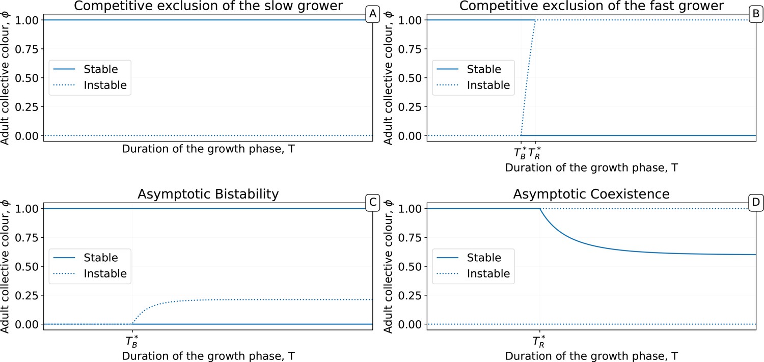
Bifurcation diagrams showing the position and stability of the fixed points of $G_{θ}$ as a function of the duration of the collective generation T.

(A-D) Particle traits are representative of the scenarios illustrated in Figure 7A–D. Of particular interest is the case illustrated in panel D, where the $G_{θ}$ function acquires — for a sufficiently large separation between the particle maximum division time and the collective generation time — a stable internal fixed point.

Appendix 2—figure 5

Download asset Open asset

Stable equilibria of the particle ecology as a function of inter-colour competition traits.

These equilibria correspond to the limit of the fixed points of the $G_{θ}$ function when particle-level and collective-level time scales are well separated ( $r ≫ \frac{1}{T}$ ), derived in proposition 3. Other interaction parameters are $a_{00} = 0.7$ and $a_{11} = 0.8$ , and the result is independent of growth rates. The grey area indicates bistability.

Appendix 2—figure 6

Download asset Open asset

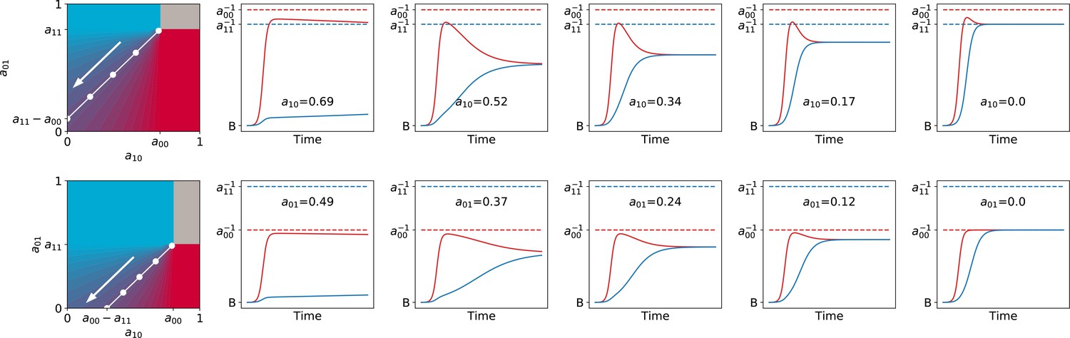
Asymmetric interaction ensures fastest convergence toward the ecological equilibrium.

Particle population dynamics are illustrated for increasingly asymmetric values of $(a_{01}, a_{10})$ , keeping the ecological equilibrium fix at $x^{*} = 0.5$ (along white manifold, in the direction of the arrow). The top panels correspond to cases when the faster-growing particles have a higher carrying capacity ( $(a_{00}, a_{11}) = (0.7, 0.8)$ ), the bottom panels to the opposite ( $(a_{00}, a_{11}) = (0.8, 0.5)$ ). In both cases $r_{0} = 60$ , $r_{1} = 40$ , $T = 1$ , $B = 0.001$ .

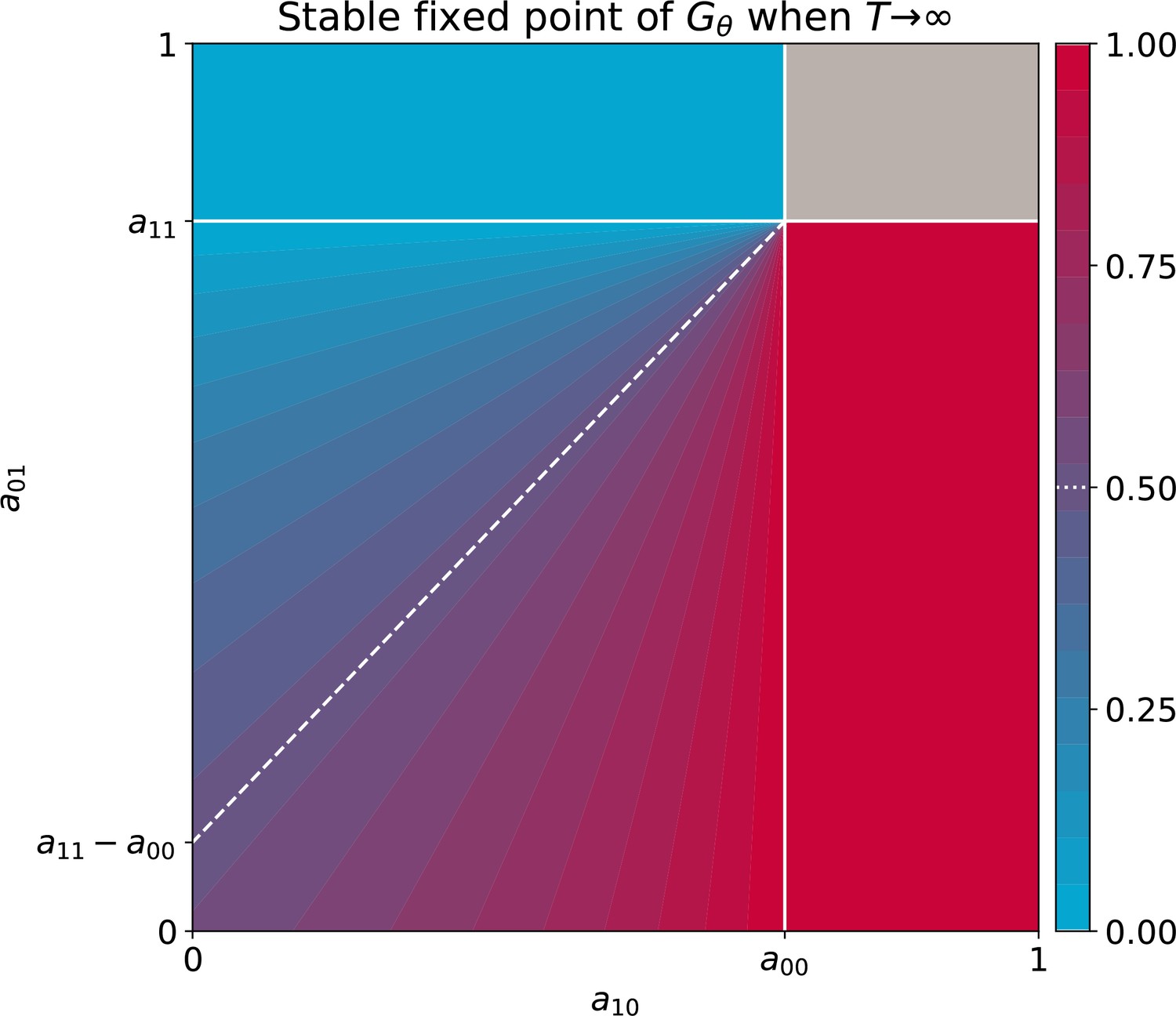
Appendix 3—figure 1

Download asset Open asset

Asymptotic colour of the particle ecology as a function of inter-colour competition traits.

These equilibria correspond to the limit of the fixed points of the $G_{θ}$ function when particle-level and collective-level time scales are well separated ( $r ≫ \frac{1}{T}$ ), derived in proposition 3. Other interaction parameters are $a_{00} = 0.7$ and $a_{11} = 0.8$ , and the result is independent of growth rates. The grey area indicates bistability. This figure extends Appendix 2—figure 5.

Appendix 3—figure 2

Download asset Open asset

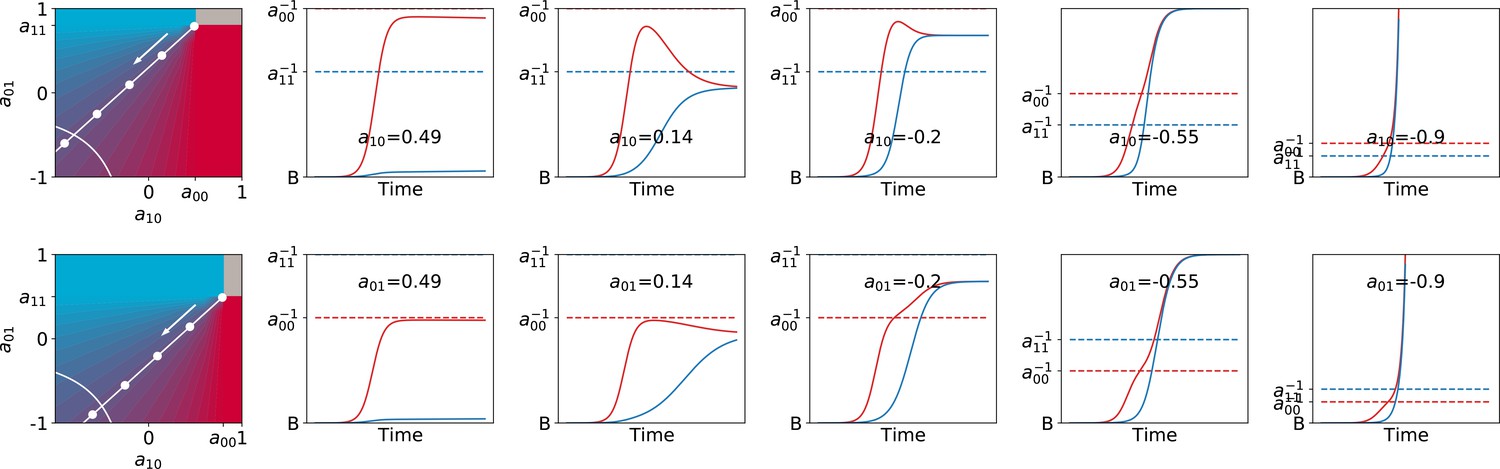
Mutualistic interaction can lead to non-saturating population growth.

Particle population dynamics are illustrated for increasingly mutualistic values of $(a_{01}, a_{10})$ , keeping the ecological equilibrium fixed at $x^{*} = 0.5$ (moving along the white manifold, in the direction of the arrow). When the determinant of $𝐀$ is negative, population growth is unbounded in the limit of infinitely long duration of the collective generation. As long as $T$ is finite, however, the adult proportion of red and blue particles can be reached even though both populations grow exponentially (with growth rates that depend on the interaction parameters). The top panels correspond to cases when the faster growing particles have a higher carrying capacity ( $(a_{00}, a_{11}) = (0.5, 0.8)$ ), the bottom panels is the opposite ( $(a_{00}, a_{11}) = (0.8, 0.5)$ ). In both cases $r_{0} = 30$ , $r_{1} = 30$ , $T = 1$ , $B = 0.001$ .

Additional files

Source code 1 Source code for simulation and figure generation. Also available at https://gitlab.com/ecoevomath/estaudel.: https://cdn.elifesciences.org/articles/53433/elife-53433-code1-v2.zip
Download elife-53433-code1-v2.zip
Transparent reporting form: https://cdn.elifesciences.org/articles/53433/elife-53433-transrepform-v2.pdf
Download elife-53433-transrepform-v2.pdf

Download links

A two-part list of links to download the article, or parts of the article, in various formats.

Downloads (link to download the article as PDF)

Article PDF

Open citations (links to open the citations from this article in various online reference manager services)

Mendeley

Cite this article (links to download the citations from this article in formats compatible with various reference manager tools)

Guilhem Doulcier
Amaury Lambert
Silvia De Monte
Paul B Rainey

(2020)

Eco-evolutionary dynamics of nested Darwinian populations and the emergence of community-level heredity

eLife 9:e53433.

https://doi.org/10.7554/eLife.53433

Sign up for email alerts

Privacy notice