Estimating and interpreting nonlinear receptive field of sensory neural responses with deep neural network models
- Department of Electrical Engineering, Columbia University, United States
- Zuckerman Mind Brain Behavior Institute, Columbia University, United States
- Feinstein Institute for Medical Research, United States
- Department of Neurosurgery, Hofstra-Northwell School of Medicine and Feinstein Institute for Medical Research, United States
Figures
Figure 1 with 2 supplements
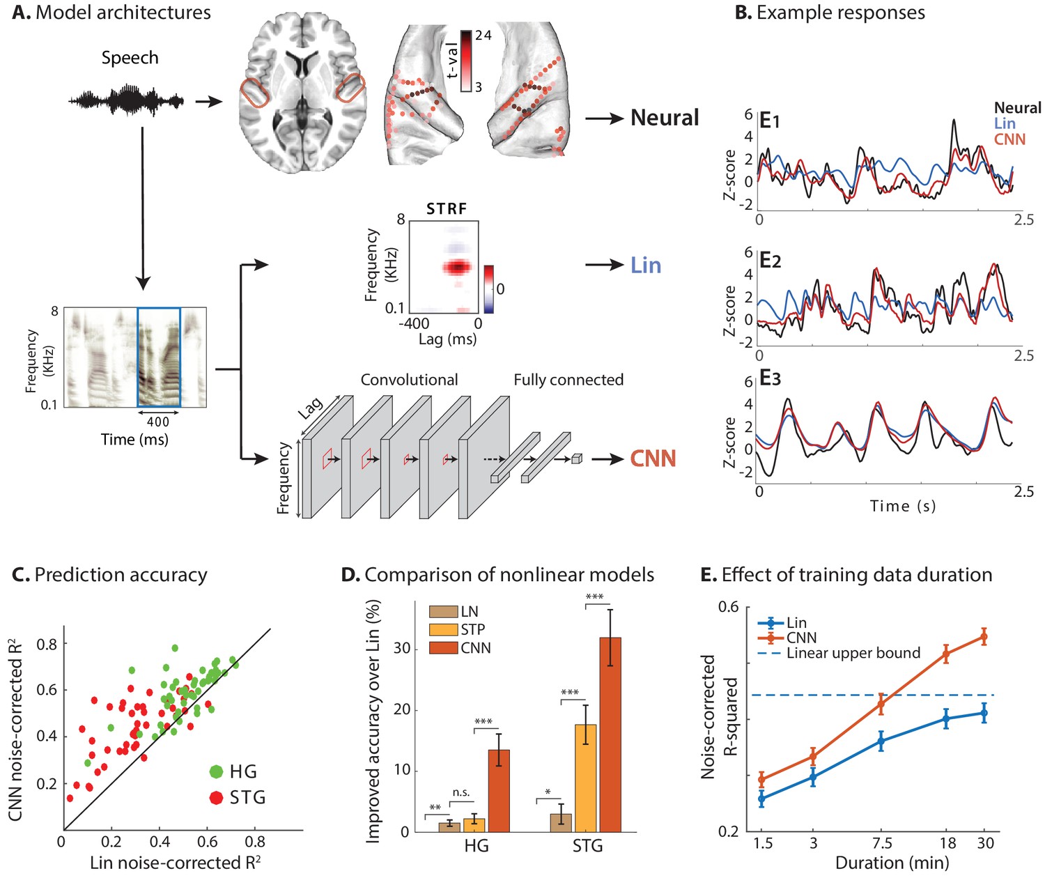
Predicting neural responses using linear and nonlinear regression models.
(A) Neural responses to speech were recorded invasively from neurosurgical patients as they listened to speech. The brain plot shows electrode locations and t-value of the difference between the average response of a neural site to speech versus silence. The neural responses are predicted from the stimulus using a linear spectrotemporal receptive field model (Lin) and a nonlinear convolutional neural network model (CNN). Input to both models is a sliding time-frequency window with 400 ms duration. (B) Actual and predicted responses of three example sites using the Lin and CNN models. (C) Prediction accuracy of neural responses from the Lin and CNN models for sites in STG and HG. (D) Improved prediction accuracy over Lin model for linear-nonlinear (LN), short-term plasticity (STP), and CNN models. (E) Dependence of prediction accuracy on the duration of training data. Circles show average across electrodes and bars indicate standard error. The dashed line is the upper bound of average prediction accuracy for the Lin model across electrodes. The x-axis is in logarithmic scale.
-
Figure 1—source data 1
A MATLAB file containing four variables — group (location of electrode based on anatomy; 1 = Heschl’s gyrus, 2 = superior temporal gyrus), rsquared_lin (noise-adjusted R-squared values of test set prediction by linear model), rqsuared_cnn (noise-adjusted R-squared values of test set prediction by CNN model), improvement (difference of the last two, as used in the Figure 5B prediction).
- https://cdn.elifesciences.org/articles/53445/elife-53445-fig1-data1-v2.mat
Figure 1—figure supplement 1
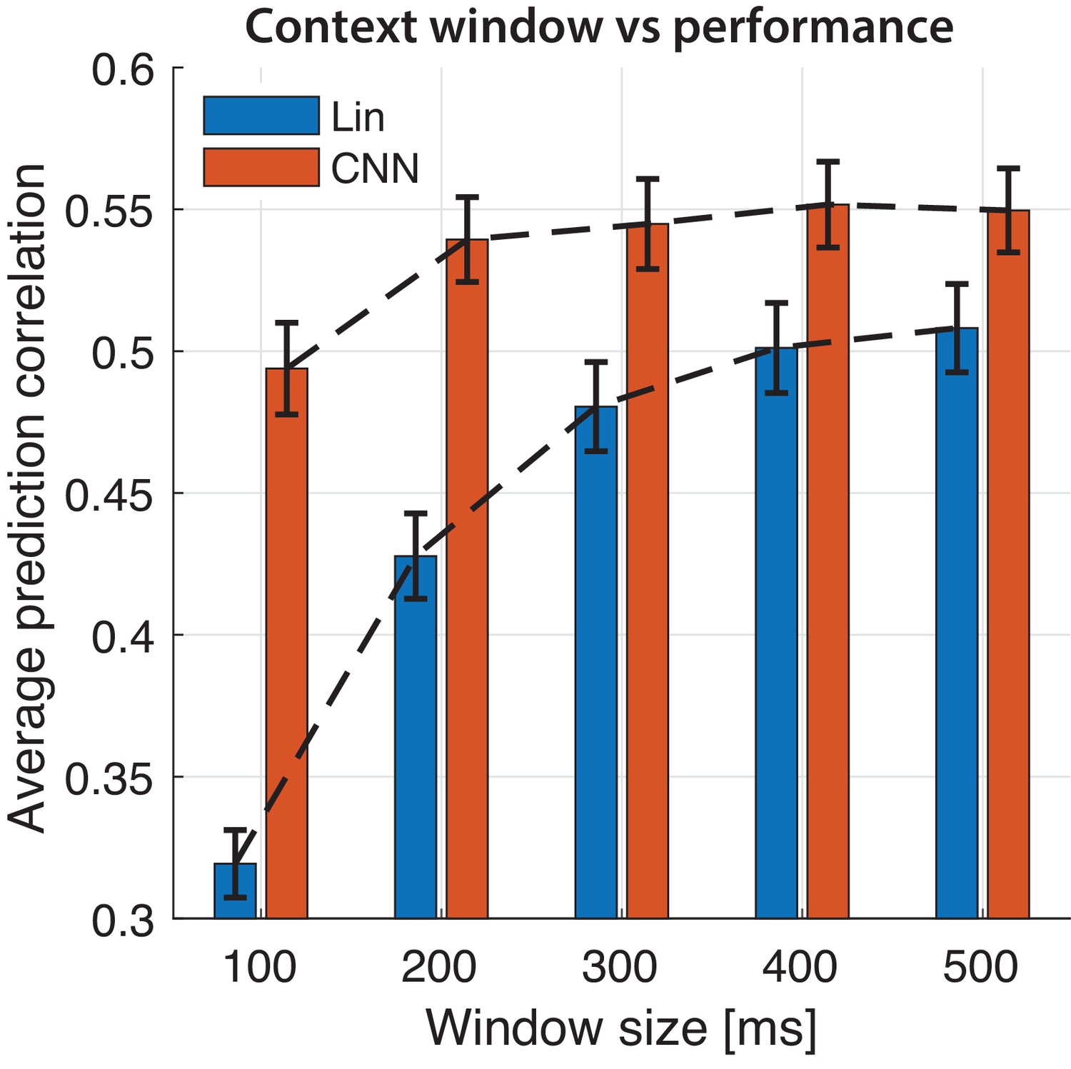
Selecting stimulus window length for prediction.
Prediction accuracy of neural responses with varying the duration of the sliding window for linear and CNN models. Bars indicate average prediction values across electrodes and error bars the standard error.
Figure 1—figure supplement 2
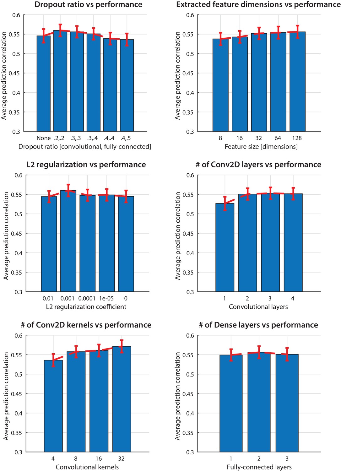
Hyperparameter optimization.
Choosing the hyperparameters of the network to maximize prediction accuracy of the CNN model. The bars indicate average prediction values across electrodes and error bars the standard error.
Figure 2 with 3 supplements

Calculating the stimulus-dependent dynamic spectrotemporal receptive field.
(A) Activation of nodes in a neural network with rectified linear (ReLU) nonlinearity for the stimulus at time . (B) Calculating the stimulus-dependent dynamic spectrotemporal receptive field (DSTRF) for input instance by first removing all inactive nodes from the network and replacing the active nodes with the identity function. The DSTRF is then computed by multiplying the remaining network weights. Reshaping the resulting weight matrix expresses the DSTRF in the same dimensions as the input stimulus and can be interpreted as a multiplicative template applied to the input. Contours indicate 95% significance (jackknife). (C) Comparison of piecewise linear (rectified linear neural network) and linear (STRF) approximations of a nonlinear function. (D) DSTRF vectors (columns) shown for 40 samples of the stimulus. Only a limited number of lags and frequencies are shown at each time step to assist visualization. (E) Normalized sorted singular values of the DSTRF matrix show higher diversity of the learned linear function in STG sites than in HG sites. The bold lines are the averages of sites in the STG and in HG. The complexity of a network is defined as the sum of the sorted normalized singular values. (F) Comparison of network complexity and the improved prediction accuracy over the linear model in STG and HG areas. (G) Histogram of the average number of switches from on/off to off/on states at each time step for the neural sites in the STG and HG.
-
Figure 2—source data 1
A MATLAB file containing one variable — complexity (neural network complexity, as used in Figure 5A prediction).
- https://cdn.elifesciences.org/articles/53445/elife-53445-fig2-data1-v2.mat
Figure 2—figure supplement 1

Converting convolution to matrix multiplication.
Converting the convolutional neural networks into a feedforward network helps simplify DSTRF calculation. The convolution operation is linear; hence, it can be converted into a matrix multiplication. (A) Converting 1-d convolution into a 2-d matrix multiplication. The matrices are the shifted version of the 1-d vectors. The -th row in the output will be the product of the input vectors (shown in green) and the convolution kernel (red) shifted by steps. (B) Converting 2-d convolution to a 2-d weight matrix using the same principle by flattening both the kernel and the input into one-dimensional forms by stacking the columns vertically on top of each other.
Figure 2—figure supplement 2
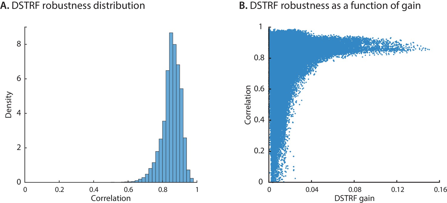
DSTRF robustness across initializations.
We trained 10 instances of the CNN model for each electrode and grouped them into two groups of evens and odds. For all time points, we calculated the 2D correlation of the average DSTRF from the even models with the average DSTRF from the odd models. (A) A histogram of all values where one data point corresponds to the robustness for a specific electrode at a specific time point. (B) The relation of robustness with the gain of the linearized function. When the DSTRF has higher gain the function is more robust.
Figure 2—figure supplement 3
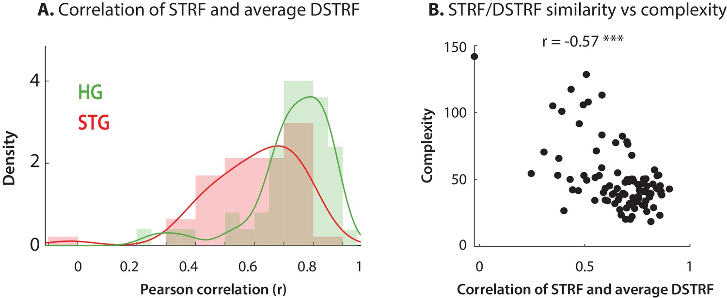
Comparing DSTRFs to STRFs.
(A) The average DSTRF calculated across the test dataset is highly correlated with the calculated STRF, especially for HG electrodes. (B) Similarity of STRF and the average DSTRF is inversely correlated with the complexity of the function the CNN model has learned, as expected. Each data point is an electrode and the R-value represents Spearman correlation.
Figure 3 with 2 supplements

Characterizing the types of DSTRF variations.
Three types of DSTRF variations are shown over time for three example sites that exhibit each of these types more prominently. The DSTRFs have been masked by 95% significance per jackknifing (). (A) The STRF of the three example sites. (B) Example site E1: Gain change of DSTRF, shown as the time-varying magnitude of the DSTRF at three different time points. Although the overall shape of the spectrotemporal receptive field is the same, its magnitude varies across time. E2: Temporal hold property of an DSTRF, seen as the tuning of this site to a fixed spectrotemporal feature but with shifted latency (lag) in consecutive time frames. E3: Shape change property of DSTRF, seen as the change in the spectrotemporal tuning pattern for different instances of the stimulus. (C) From top to bottom, distribution of gain change, temporal hold, and shape change values for sites in HG and STG. Horizontal lines mark quartiles. Temporal hold and shape change show significantly higher values in the STG.
-
Figure 3—source data 1
A MATLAB file containing three variables, one for each type of quantified nonlinearity — nonlin_gain_change (gain change nonlinearity), nonlin_temporal_hold (temporal hold nonlinearity), nonlin_shape_change (shape change nonlinearity).
- https://cdn.elifesciences.org/articles/53445/elife-53445-fig3-data1-v2.mat
Figure 3—figure supplement 1
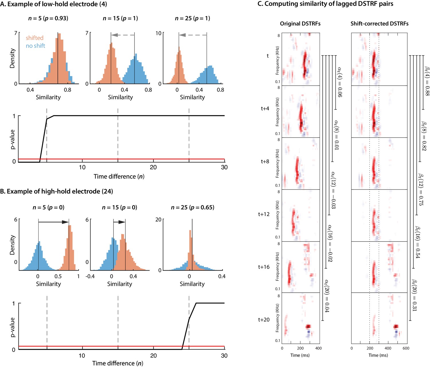
Calculating temporal hold.
(A, B) shows the procedure used for calculating temporal hold for two example electrodes. The first row in each panel shows the distributions for DSTRF pair similarities when shifted () and without shift () for all as described in the methods for three distinct values of time difference between compared DSTRF pairs (), along with their respective p-values from the one-tailed signed-rank test. The second row shows the p-values for all . The red horizontal line indicates the threshold . (C) demonstrates how DSTRF samples are shifted and compared with each other to obtain and .
Figure 3—figure supplement 2

Nonlinearity robustness to initialization and data.
(A) We trained 10 instances of the CNN model for each electrode and grouped them into two groups of evens and odds. We measured the three nonlinearity parameters from the average DSTRFs of each group on the test dataset, and compared the values from the two conditions. (B) We measured the three nonlinearity parameters independently from two splits of the test dataset, and compared the values from the two conditions. The R-values represent Spearman correlation.
Figure 4

Characterizing the spectrotemporal tuning of electrodes with clustering.
(A, B) The average shift-corrected DSTRF for two example sites and average k-means clustered DSTRFs based on the similarity of DSTRFs (correlation distance). Each cluster shows tuning to a distinct spectrotemporal feature. The average DSTRF shows the sum of these different features. The average spectrograms over the time points at which each cluster DSTRF was selected by the network demonstrate the distinct time-frequency pattern in the stimuli that caused the network to choose the corresponding template.
Figure 5 with 2 supplements
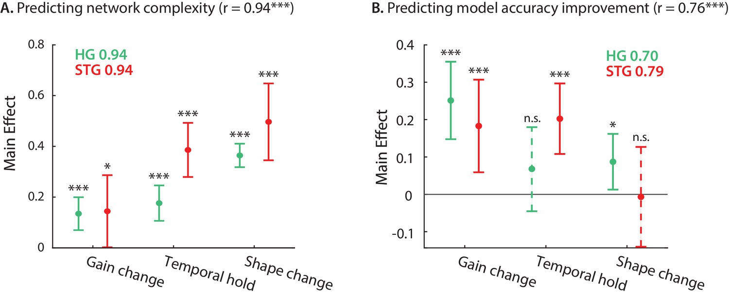
Contribution of DSTRF variations to network complexity and prediction improvement.
(A) Predicting the complexity of the neural networks from gain change, temporal hold, and shape change using a linear regression model. The main effect of regression analysis shows the significant contribution of all nonlinear parameters in predicting the network complexity in both STG and in HG sites. Legend shows prediction R-values separately for each region. (B) Predicting the improved accuracy of neural networks over the linear model from the three nonlinear parameters for each site in the STG and HG. The main effect of the regression analysis shows different contribution of the three nonlinear parameters in predicting the improved accuracy over the linear model in different auditory cortical areas. Figure legends shows prediction R-values separately for each region.
Figure 5—figure supplement 1

Complexity and accuracy improvement predicted values.
True and predicted values for network complexity and improved model accuracy from the three nonlinear parameters.
Figure 5—figure supplement 2
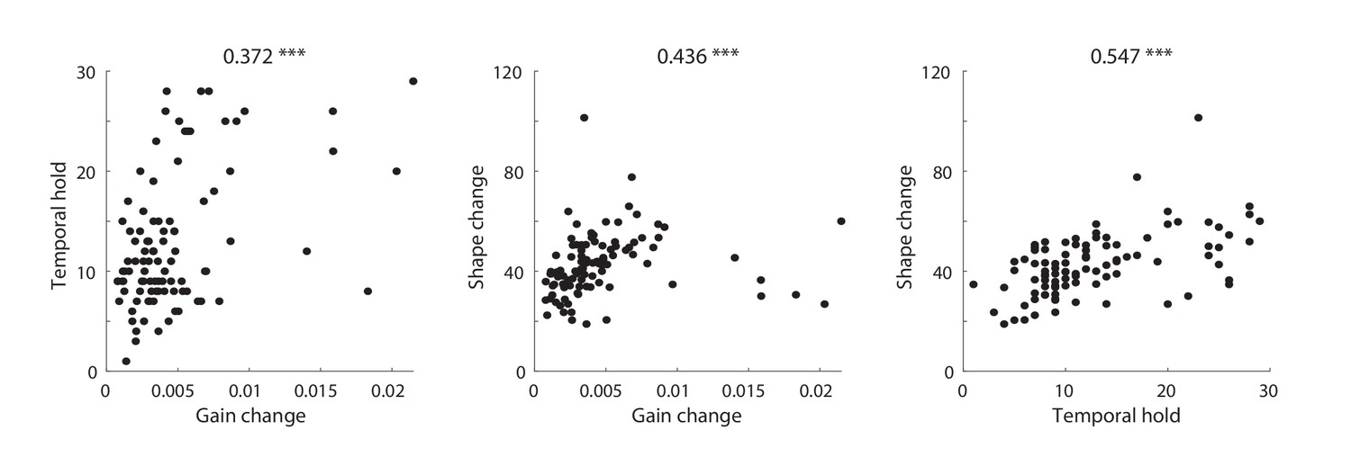
Covarying nonlinear parameters.
The three parameters characterizing the nonlinear properties of neural sites (gain change, temporal hold, and shape change) are not independent and covary significantly. The values represent Spearman correlation.
Videos
Video 1
The spectrotemporal receptive field (STRF) model applies a weight function to the stimulus to predict the neural response.
Video 2
The dynamic spectrotemporal receptive field (DSTRF) applies a time-varying, stimulus-dependent weight function to the stimulus to predict the neural response.
Video 3
Visualization of gain change, temporal hold, and shape change for three example electrodes, each demonstrating one type of nonlinearity more prominently.
Additional files
Download links
A two-part list of links to download the article, or parts of the article, in various formats.
Downloads (link to download the article as PDF)
Open citations (links to open the citations from this article in various online reference manager services)
Cite this article (links to download the citations from this article in formats compatible with various reference manager tools)
Estimating and interpreting nonlinear receptive field of sensory neural responses with deep neural network models
eLife 9:e53445.
https://doi.org/10.7554/eLife.53445


