Synteny-based analyses indicate that sequence divergence is not the main source of orphan genes
- Trinity College Dublin, University of Dublin, Ireland
- University of Pittsburgh, United States
Figures
Figure 1
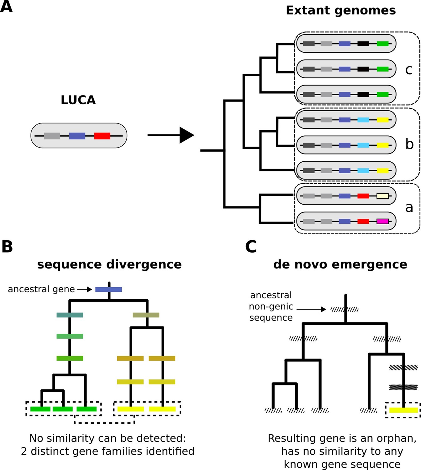
From a limited set of genes in LUCA to the multitudinous extant patterns of presence and absence of genes.
(A) Cartoon representation of the LUCA gene repertoire and extant phylogenetic distribution of gene families (shown in different colours, same colour represents sequence similarity and homology). Dashed boxes denote different phylogenetic species groups. Light grey and dark blue gene families cover all genomes and can thus be traced back to the common ancestor. Other genes may have more restricted distributions; for example, the yellow gene is only found in group b, the black gene in group c. The phylogenetic distribution of gene family members allows us to propose hypotheses about the timing of origination of each family. (B) Sequence divergence can gradually erase all similarity between homologous sequences, eventually leading to their identification as distinct gene families. Note that divergence can also occur after a homologous gene was acquired by horizontal transfer. Solid boxes represent genes. Sequence divergence is symbolized by divergence in colour. (C) De novo emergence of a gene from a previously non-genic sequence along a specific lineage will almost always result in a unique sequence in that lineage (cases of convergent evolution can in theory occur). Hashed boxes represent non-genic sequences.
Figure 2 with 1 supplement

Summary of the main concept and pipeline of identification of putative homologous pairs with undetectable similarity between pairs of genomes.
(A) Summary of the reasoning we use to estimate the proportion of genes in a genome that have diverged beyond recognition. (B) Pipeline of identification of putative homologous pairs with undetectable similarity. 1) Choose focal and target species. Parse gene order and retrieve homologous relationships from OrthoDB for each focal-target pair. Search for sequence similarity by BLASTP between focal and target proteomes, one target proteome at a time. 2) For every focal gene (b), identify whether a region of conserved micro-synteny exists, that is when the upstream (a) and downstream (c) neighbours have homologues (a’, c’) separated by either one or two genes. This conserved micro-synteny allows us to assume that b and b’ are most likely homologues. Only cases for which the conserved micro-synteny region can be expanded by one additional gene are retained. Specifically, if genes d and e have homologues, these must be separated by at most one gene from a’ and c’, respectively. A per-species histogram of the number of genes with at least one identified region of conserved micro-synteny can be found in Figure 2—figure supplement 1. For all genes where at least one such configuration is found, move to the next step. 3) Check whether a precalculated BLASTP hit exists (by our proteome searches) between query (b) and candidate homologue (b’) for a given E-value threshold. If no hit exists, move to the next step. 4) Use TBLASTN to search for similarity between the query (b) and the genomic region of the conserved micro-synteny (-/+ 2 kb around the candidate homologue gene) for a given E-value threshold. If no hit exists, move to the next step. 5) Extend the search to the entire proteome and genome. If no hit exists, move to the next step. 6) Record all relevant information about the pairs of sequences forming the b – b’ pairs of step 2). Any statistically significant hit at steps 3–5 is counted as detected homology by sequence similarity. In the end, we count the total numbers of genes in conserved micro-synteny without any similarity for each pair of genomes.
Figure 2—figure supplement 1

Total number of genes in the focal species genome for which a region in conserved micro-synteny was identified in a given target species (x axis).
Species are ordered in increasing divergence times from their corresponding focal species.
Figure 3
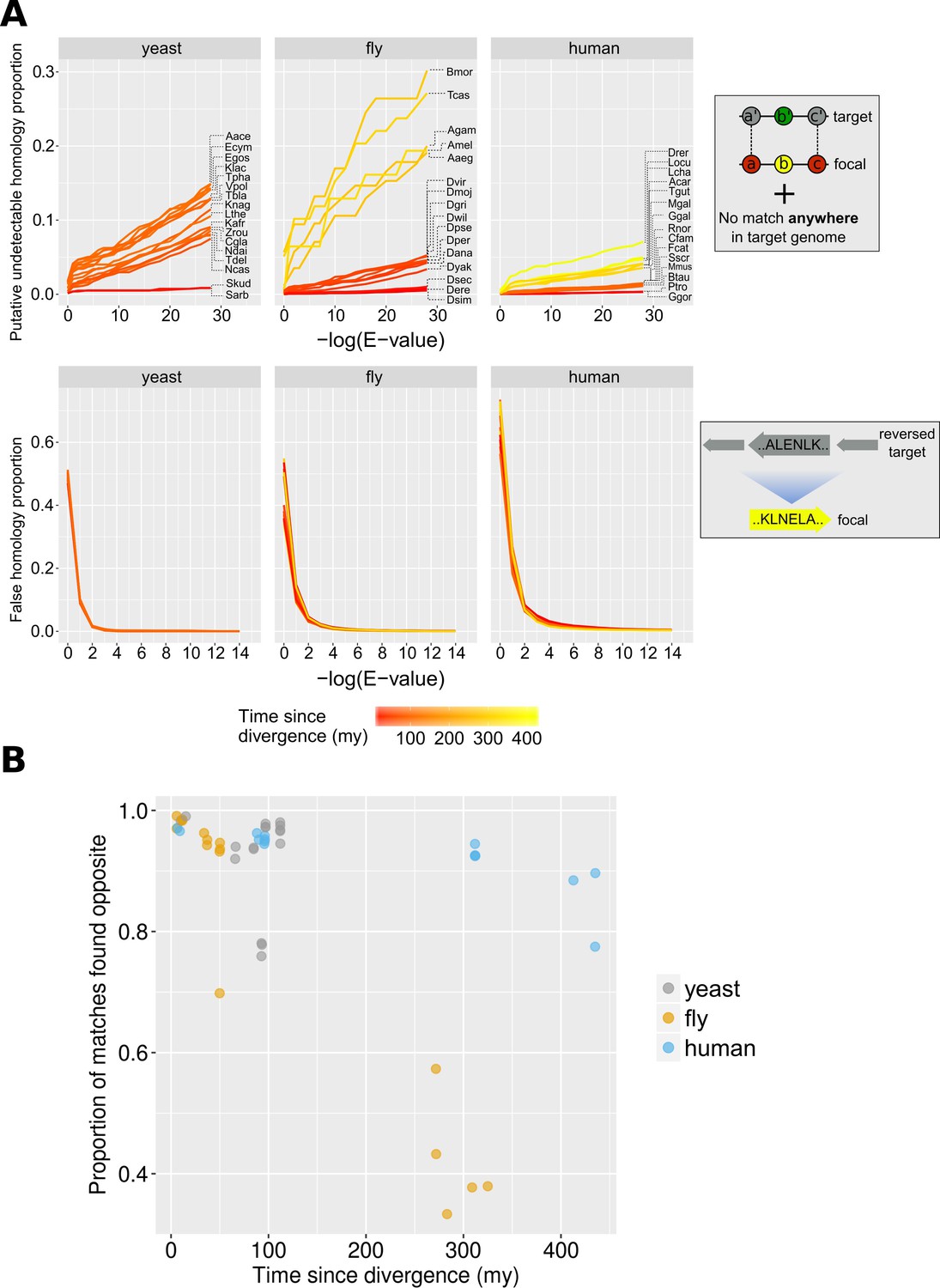
Proportions of false and undetectable homologies for a range of E-value cut-offs.
(A) Proportions of false and undetectable homologies as a function of the E-value cut-off used. Abbreviations of species names can be found in Table 1. Putative undetectable homology proportion (top row) is defined as the percentage of all genes with at least one identified region of conserved micro-synteny (and thus likely to have a homologue in the target genome) that have no significant match anywhere in the target genome (see Materials and methods and Figure 2). False homology proportion (bottom row) is defined as a significant match to the reversed proteome of the target species (see Materials and methods). Divergence time estimates were obtained from www.TimeTree.org. Data for this figure can be found in Figure 3—source data 2 (upper plots) and Figure 3—source data 3 (lower plots). (B) Proportion (out of all genes with sequence matches) where a match is found in the predicted region (‘opposite’) in the target genome for the three datasets, using the relaxed E-value cut-offs (0.01, 0.01, 0.001 for yeast, fly and human, respectively [10−4 for comparison with chimpanzee]), as a function of time since divergence from the respective focal species. Data can be found in Figure 3—source data 1.
-
Figure 3—source data 1
Data from focal-target genome comparisons.
‘div. time’: time since divergence from the focal species. ‘Phylostrat. E-value’: optimal E-value for use in phylostratigraphy. ‘general E-value’: optimal E-value maximizing Mathews Correlation Coefficient. ‘# residues’: number of residues in the complete proteome of the species. ‘found opposite’: genes in conserved micro-synteny whose sequence match is found at the predicted genomic location. ‘found elsewhere’: genes in conserved micro-synteny whose match is found elsewhere than the predicted location. ‘not found (and in micro-synteny)': genes in conserved micro-synteny that do not have a match. ‘total in micro-synteny’: total number of genes in conserved micro-synteny. ‘not found and outside micro-synteny’: number of genes without a match that are not found in conserved micro-synteny. ‘total genes checked’: number of focal genes examined.
- https://cdn.elifesciences.org/articles/53500/elife-53500-fig3-data1-v1.csv
-
Figure 3—source data 2
Data on undetectable homologies for different E-value cut-offs used to generate the top panel of Figure 3A.
Column names: ‘total’: total number of genes in conserved micro-synteny, ‘not_found’: number of genes without significant sequence similarity, ‘div’: time since divergence from focal species.
- https://cdn.elifesciences.org/articles/53500/elife-53500-fig3-data2-v1.csv
-
Figure 3—source data 3
Data on false homologies for different E-value cut-offs used to generate the bottom panel of Figure 3A.
Column names: ‘found’: number of genes with significant sequence similarity, the rest are the same as in Source Data 1.
- https://cdn.elifesciences.org/articles/53500/elife-53500-fig3-data3-v1.csv
Figure 4 with 1 supplement
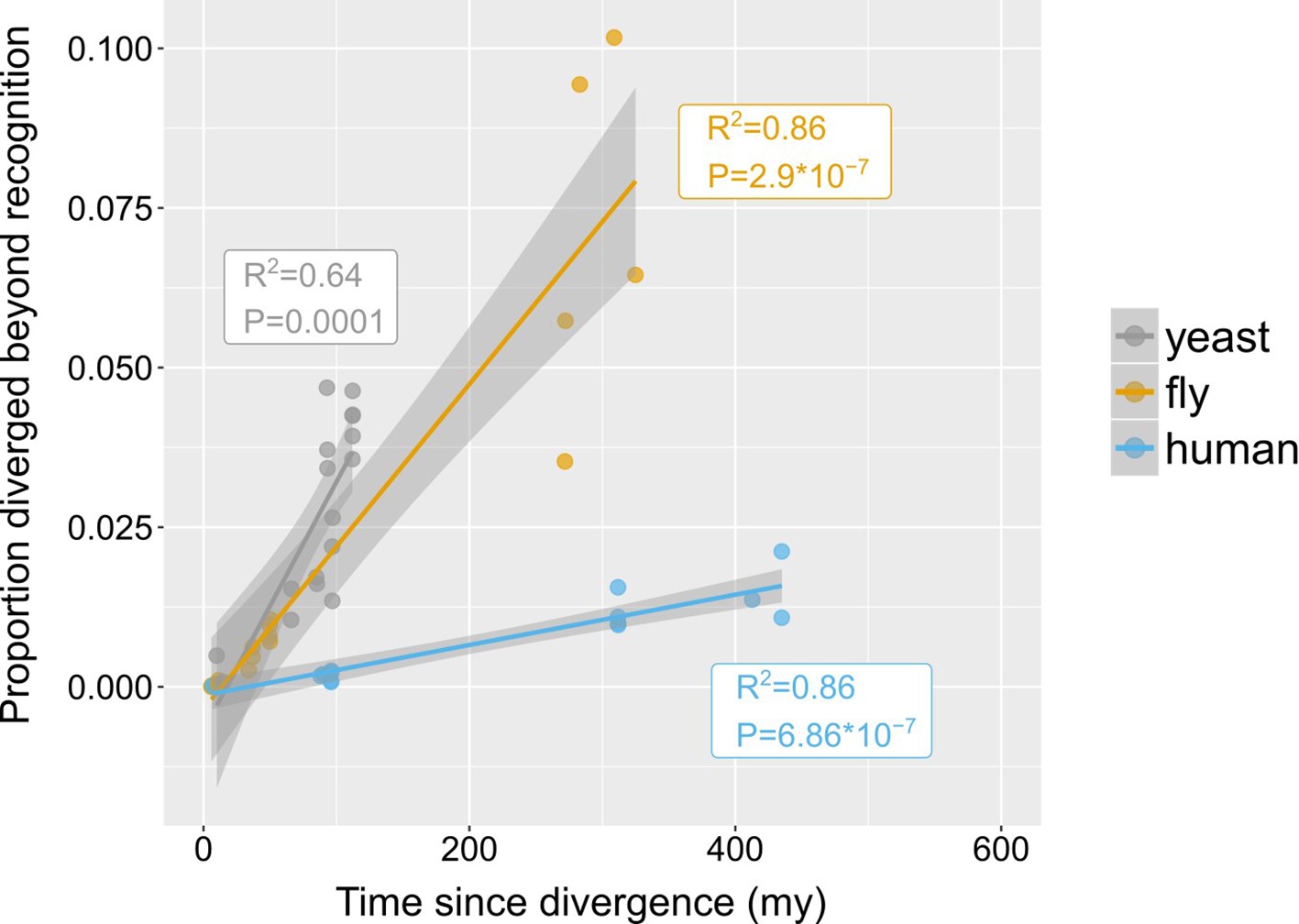
Rates of divergence beyond recognition.
Putative undetectable homology proportion in focal - target species pairs plotted against time since divergence of species. The y axis represents the proportion of focal genes in micro-synteny regions for which a homologue cannot be detected by similarity searches in the target species. Linear fit significance is shown in the graph. Points have been jittered along the X axis for visibility. Two exemplars of focal-target undetectable homologues can be found in Figure 4—figure supplement 1. Data can be found in Figure 3—source data 1.
Figure 4—figure supplement 1

Two examples of putative homologues diverged beyond recognition.
(A) Genomic region comparison view of ENSEMBL for the case of the human gene CSAG1 (top) and its undetectable homologue in mouse, 1700084M14Rik (bottom). The two genes are highlighted in green, while the adjacent genes based on which the syntenic region was defined are highlighted in blue rectangles. (B) Same as in A but for the D. melanogaster gene CG13577 (top) and its undetectable homologue in D. virilis DvirGJ21588. Note that this is not a genomic region comparison view, but two separate genome browser views from the ENSEMBL metazoan web resource.
Figure 5
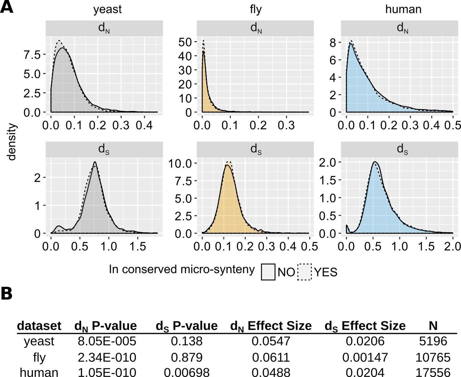
Comparison of evolutionary rates between genes inside and outside conserved micro-synteny regions.
(A) Density plots of dS and dN distributions. Outliers are not shown for visual purposes Data can be found in Figure 5—source data 1. (B) Statistics of unpaired Wilcoxon test comparisons between genes inside and outside of conserved micro-synteny. Effect size was calculated using Rosenthal’s formula (Rosenthal et al., 1994) (Z/sqrt(N)).
-
Figure 5—source data 1
dN and dS data used to generate Figure 5 and the accompanying statistics.
See Materials and methods section for how these data were generated. Column names: ‘micro-synteny’: whether the gene satisfies our conserved micro-synteny criteria with the relevant species (see Materials and methods).
- https://cdn.elifesciences.org/articles/53500/elife-53500-fig5-data1-v1.csv
Figure 6 with 3 supplements
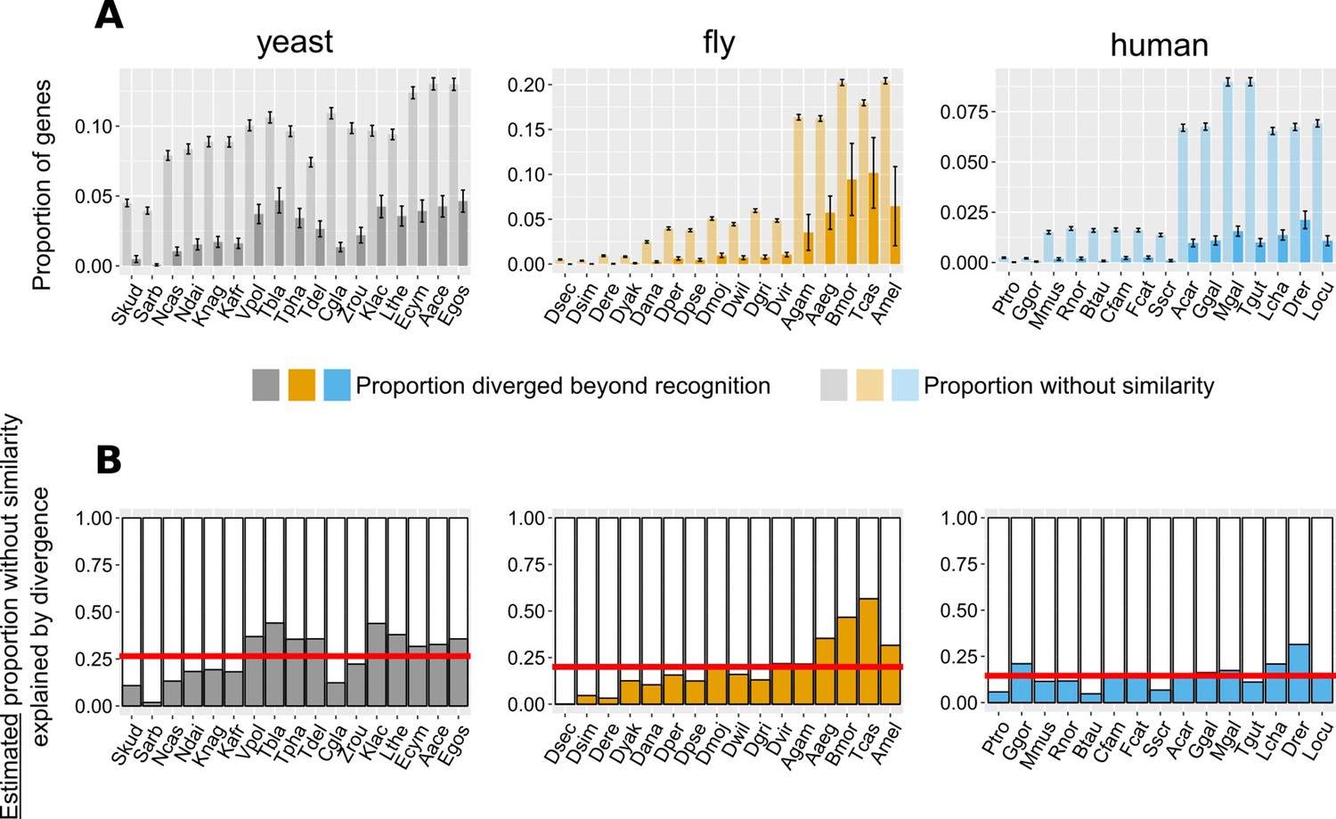
Contribution of divergence beyond recognition to observed numbers of genes without detectable similarity.
(A) Proportion of genes with undetectable homologues in micro-synteny regions (thus likely diverged beyond recognition, solid bars) and proportion of total genes without similarity, genome-wide (transparent bars), in the different focal - target genome pairs. Schematic representation for how these proportions are calculated can be found in Figure 6—figure supplement 1. Error bars show the standard error of the proportion. (B) Estimated proportions of genes with putative undetectable homologues (explained by divergence) out of the total number of genes without similarity genome-wide. This proportion corresponds to the ratio of the micro-synteny proportion (solid bars in top panel) extrapolated to all genes, to the proportion calculated over all genes (transparent bars in top panel). See text for details. Red horizontal lines show averages. Species are ordered in ascending time since divergence from the focal species. Abbreviations used can be found in Table 1. The equivalent results using the phylogeny-based approach can be found in Figure 6—figure supplement 3. The impact of more/less stringent conserved synteny definitions on this result can be found in Figure 6—figure supplement 2 (see also Materials and methods for details). Data for this figure and for Figure 6—figure supplement 3 can be found in Figure 6—source data 1.
-
Figure 6—source data 1
Excel file with one dataset per sheet, containing the similarity and micro-synteny conservation information for every focal - target species comparison.
- https://cdn.elifesciences.org/articles/53500/elife-53500-fig6-data1-v1.xlsx
Figure 6—figure supplement 1

Schematic representation of a toy example as an aid to understand how the proportion of genes without similarity that is explained by divergence is estimated.
Horizontal lines represent segments of chromosomes, and circles represent genes. Checkmarks denote identified sequence similarity. Red 0’s denote absence of sequence similarity. n: number of total genes; X: number of genes without sequence similarity; F: focal genome; T: target genome. Blue shades represent sequence similarity searches. In the upper part of the figure, we represent the similarity search at the entire proteome level between focal and target genomes. In the lower part of the figure, we indicate the analysis within conserved micro-synteny regions, where dashed lines indicate homologues used to define micro-synteny conservation. For the gene of interest (yellow circles in the focal genome) sequence similarity in the target genome is indicated by shared colour of circles.
Figure 6—figure supplement 2
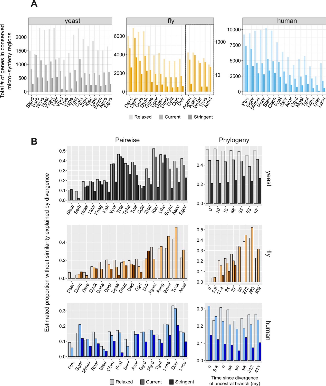
Impact of the definition of conserved micro-synteny to proportion explained by divergence.
(A) Total number of genes in conserved micro-synteny regions using three different definitions of conserved synteny blocks: ‘relaxed’: only one syntenic homologous gene on either side; ‘current’: the definition used throughout our manuscript, which is more stringent than the ‘relaxed’ one; ‘stringent’: three syntenic homologous genes on either side, or two syntenic homologues if the −3, +3 neighbours have no homologues at all (see Materials and methods for details). The five most distant species in the fly dataset are shown on a separate, logarithmic scale for visual purposes, since the ‘stringent’ definition greatly reduces the number of identified conserved regions. Notice that this is true as well in other cases, such as for ‘Vpol’ and ‘Tbla’ in the yeast dataset. (B) Estimated ‘proportions explained by divergence’ for the pairwise (left) and the phylogeny-based (right) approaches, using three different definitions of conserved synteny blocks (explained in A). Note that the ‘relaxed’ definition introduces some known false positives (non-homologous genes which due to rearrangements are placed ‘opposite’ each other), and it is for this reason that the current definition was eventually preferred (see Materials and methods for more details). As expected from the presence of these false positives the results show a limited increase but are generally similar: pairwise overall mean 23% (relaxed) vs. 20.6% (current), phylogeny-based overall mean 33.7% (relaxed) vs. 30% (current). The ‘stringent’ definition becomes problematic in many cases, especially in the comparison of distant species, as the number of genes for which the synteny criterion is satisfied becomes too small (as shown in A). A comparison including only species with >200 conserved micro-synteny regions (i.e. excluding ‘Vpol’, ‘Tbla’, ‘Tpha’, ‘Ecym’, ‘Agam’, ‘Aaeg’, ‘Bmor’, ‘Tcas’, ‘Amel’, ‘Drer’) shows that in the pairwise case the mean drops from 16% in the current one to 10.9% in the stringent one. Applying the same cut-off in the phylogeny-based case (meaning that we exclude the four more distant phylostrata of the fly dataset), we get an average of 14% for stringent compared to 27.4% for current.
Figure 6—figure supplement 3
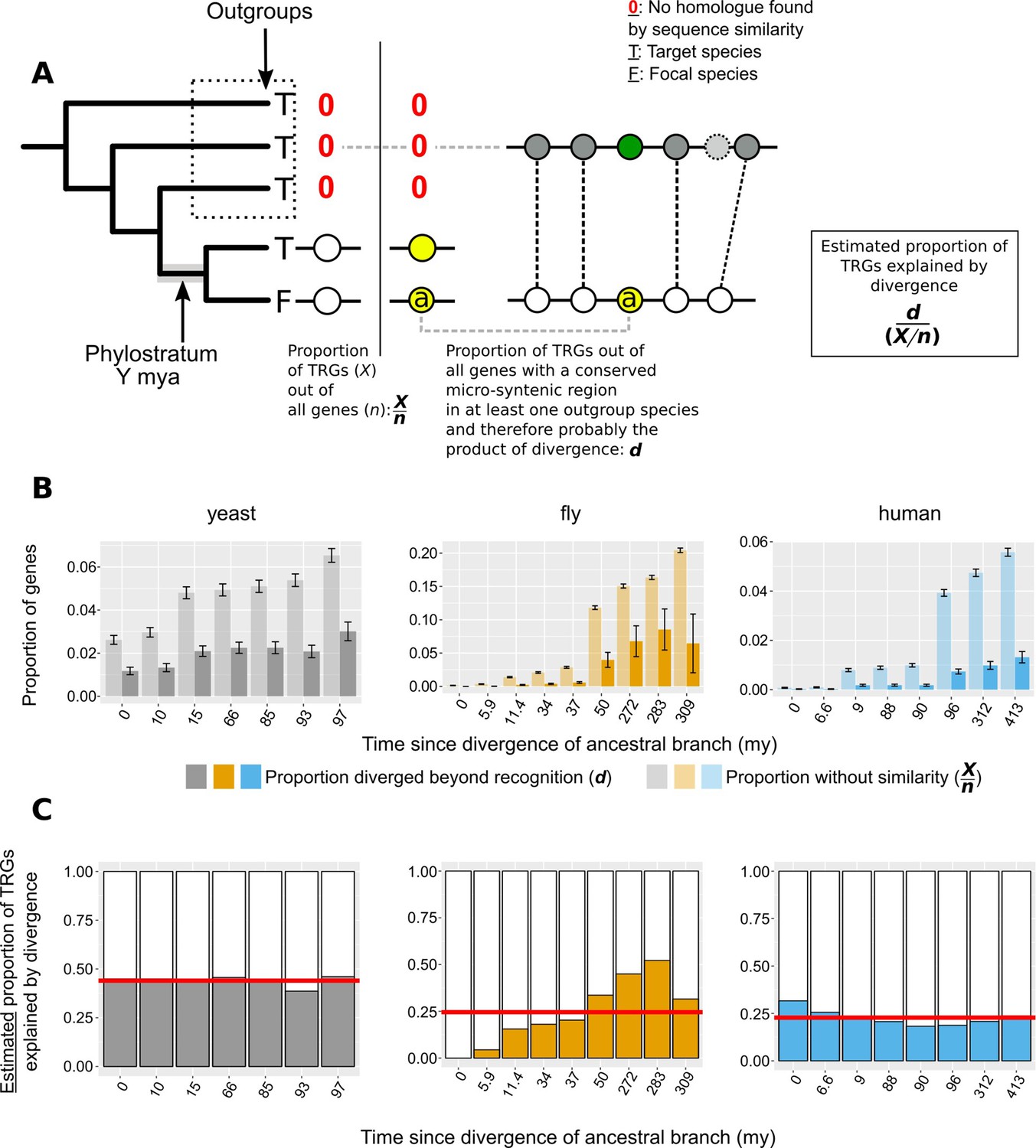
Phylogeny-based approach to estimate the contribution of divergence to TRGs.
(A) n: number of total genes; X: number of Taxonomically Restricted Genes (TRGs). Graphical representation of the of the phylogeny-based approach to estimate the proportion of genes that lack similarity beyond a specific phylogenetic level because of sequence divergence. The phylogenetic tree on the left-hand side of the vertical line shows an example of a TRG: a focal species (F) gene that has a homologue (defined by sequence similarity) only in its closest neighbour and nowhere else (absence of homologue is shown with a red 0). This permits the inference of the branch origin of this gene (phylostratum of the gene) as the branch just prior to the divergence of the lineages that carry the gene (highlighted in grey). For each phylostratum we can calculate the proportion of genes originated since (X) out of all genes in the genome (n). On the right-hand side of the vertical line we show an example of a gene (a) that is also a TRG as in the left-hand side, but that also has a region of conserved micro-synteny with a species outside of the phylostratum, that is an outgroup. Thus, we can infer that this TRG can be explained by sequence divergence, as it appears to have an undetectable homologue in one of the outgroups. Similarly to the pairwise case then, we can calculate the proportion of TRGs explained by divergence (d) as the number of such cases (TRGs with conserved micro-synteny with at least one outgroup and hence a putative undetectable homologue in an outgroup) out of all the genes with conserved micro-synteny with at least one outgroup. (B) Same as Figure 6A but with phylostrata. For each phylostratum, transparent bars show the proportion X/n as defined above in A and solid bars the proportion d. (C) Same as Figure 6B but with phylostrata. For each phylostratum, the ratio of the two proportions shown in top panel (d/[X/n]), for which we have assumed that proportion d, calculated over genes showing conserved micro-synteny with an outgroup, can be approximately extrapolated genome-wide. This ratio gives the estimated proportion of TRGs explained by divergence. Red horizontal lines show averages.
Figure 7
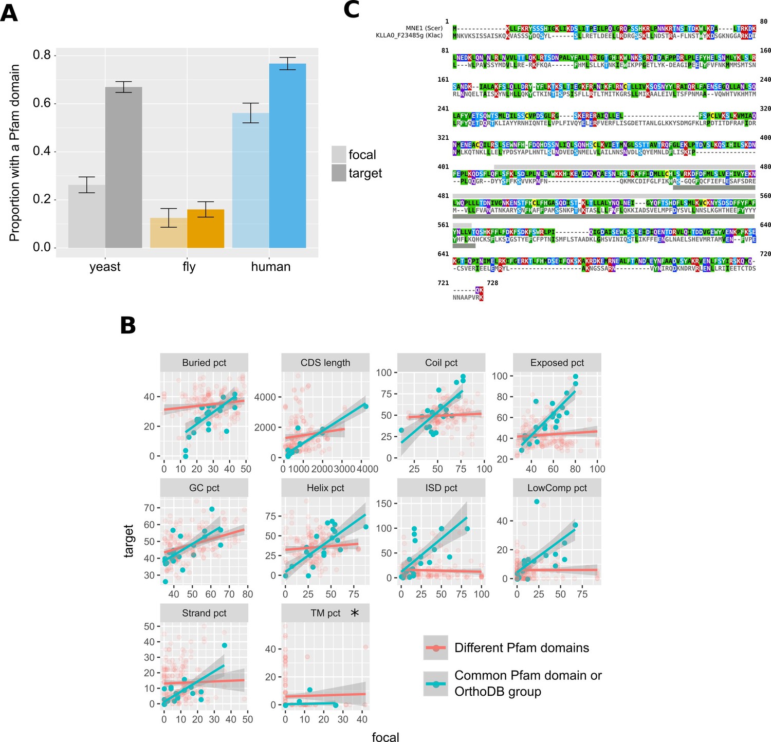
Pfam domains and other protein properties across undetectable homologue pairs.
(A) Pfam domain matches in undetectable homologues. ‘focal’ (transparent bars) corresponds to the genes in the focal species, while ‘target’ (solid bars) to their putative undetectable homologues in the target species. Whiskers show the standard error of the proportion. The yeast comparison is statistically significant at p-value<2.2×10⁻¹⁶ and the human comparison at p-value=2×10⁻⁵ (Pearson’s Chi-squared test). Raw numbers can be found in Figure 7—source data 2. (B) Distributions of properties of focal genes (‘focal’) and their undetectable homologues (‘target’), when both have a significant match (p-value<0.001) to a Pfam domain or are members of the same OrthoDB group (blue points; n = 25), and when they lack a common Pfam match but both have at least one (red points; n = 183). All blue points correlations are statistically significant (Spearman’s correlation, p-value<0.05; Bonferroni corrected) except from percentage of transmembrane residues (TM pct), marked with an asterisk. Details of correlations can be found in Figure 7—source data 1. All units are in percentage of residues, apart from ‘GC pct’ (nucleotide percentage) and CDS length (nucleotides). ‘Buried pct’: percentage of residues in regions with low solvent accessibility; ‘CDS length’: length of the CDS; ‘Coil pct’: percentage of residues in coiled regions; ‘Exposed pct’: percentage of residues in regions with high solvent accessibility; ‘GC pct’: Guanine Cytosine content; ‘Helix pct’: percentage of residues in alpha helices; ‘ISD pct’: percentage of residues in disordered regions; ‘LowComp pct’: percentage of residues in low complexity regions; ‘Strand pct’: percentage of residues in beta strands; ‘TM pct’: percentage of residues in transmembrane domains. Data can be found in Figure 7—source data 3. (C) Protein sequence alignment generated by MAFFT of MNE1 and its homologue in K. lactis. Pfam match location is shown with a light grey rectangle in S. cerevisiae, and a dark grey one in K. lactis.
-
Figure 7—source data 1
Correlations of different protein properties between undetectable homologues.
Full property names can be found in the legend of Figure 7.
- https://cdn.elifesciences.org/articles/53500/elife-53500-fig7-data1-v1.csv
-
Figure 7—source data 2
Numbers of focal and target genes with Pfam matches and total numbers.
- https://cdn.elifesciences.org/articles/53500/elife-53500-fig7-data2-v1.csv
-
Figure 7—source data 3
Data on common Pfam matches and gene/protein properties used to generate Figure 7.
Column names: ‘Gene_focal’: Name of the focal species gene, ‘Gene_ortho’: name of the target species gene, ‘same’: whether a common Pfam match was found or these genes are in the same OrthoDB group, ‘focal’: the value for the property in the focal gene, ‘ortho’: the value for the property in the target species gene, ‘var’: the name of the property.
- https://cdn.elifesciences.org/articles/53500/elife-53500-fig7-data3-v1.csv
Figure 8
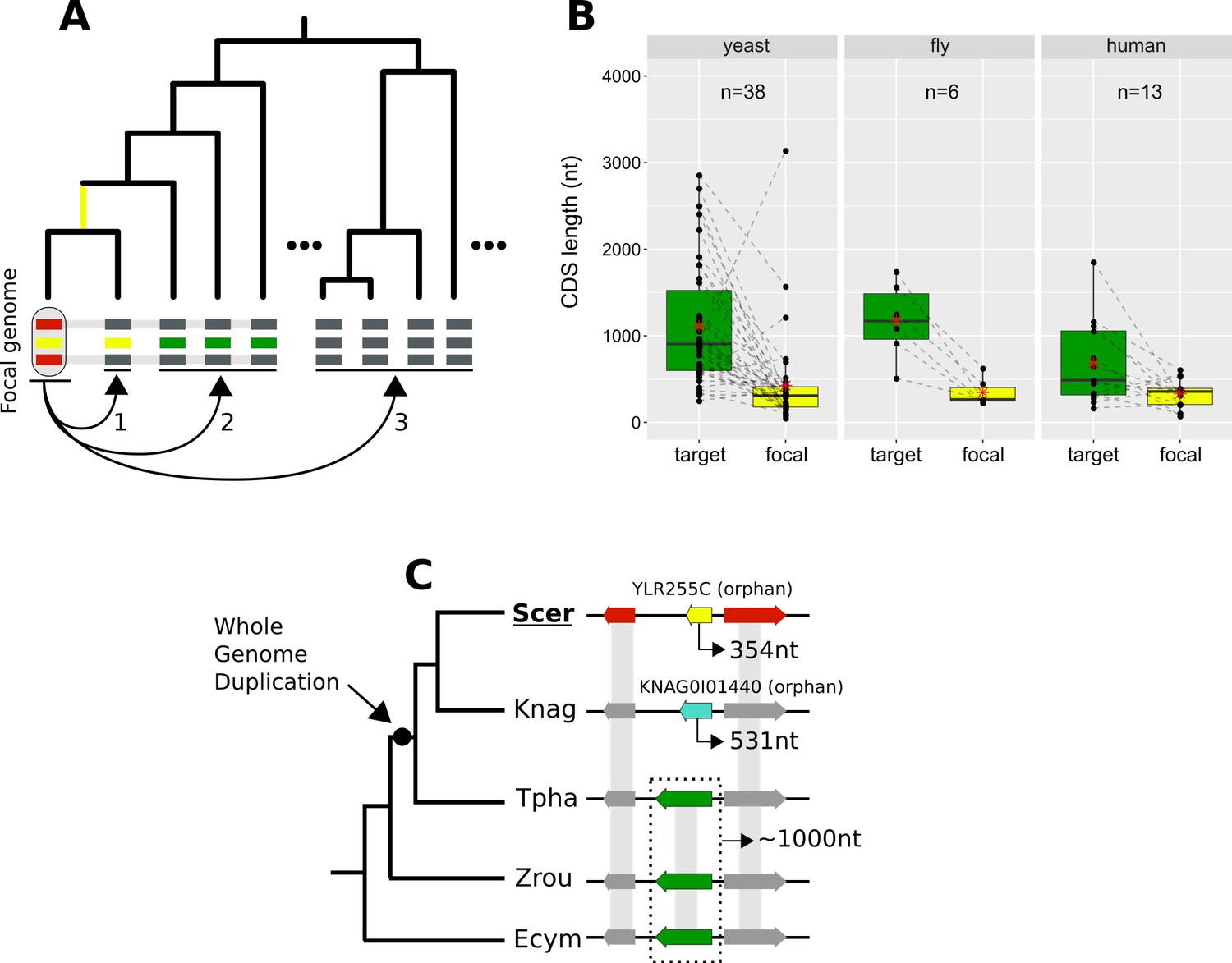
Lineage-specific divergence and gene length.
(A) Schematic representation of the criteria used to detect lineage-specific divergence. 1, identification of any lineages where a homologue with a similar sequence can be detected (example for one lineage shown). 2, identification of at least two non-monophyletic target species with an undetectable homologue. 3, search in proteomes of outgroup species to ensure that no other detectable homologue exists. The loss of similarity can then be parsimoniously inferred as having taken place, through divergence, approximately at the common ancestor of the yellow-coloured genes (yellow branch). Leftmost yellow box: focal gene; Red boxes: neighbouring genes used to establish conserved micro-synteny; Green boxes: undetectable homologues. Grey bands connecting genes represent homology identifiable from sequence similarity. (B) CDS length distributions of focal genes and their corresponding undetectable homologues (averaged across all undetectable homologous genes of each focal one) in the three datasets. Dashed lines connect the pairs. All comparisons are statistically significant at p-value<0.05 (Paired Student’s t-Test P-values: 2.5×10⁻⁵, 0.0037, 0.03 in yeast, fly and human respectively). Distribution means are shown as red stars. Box colours correspond to coloured boxes representing genes in A, but only the focal genome gene (leftmost yellow gene in A) is included in the ‘focal’ category. Data can be found in Figure 8—source data 1. All focal-target undetectable homologue pairs (not just the ones included in this figure) can be found in Figure 8—source data 2. (C) Schematic representation of the species topology of 5 yeast species (see Table 1 for abbreviations) and the genic arrangements at the syntenic region of YLR255C (shown at the ‘Scer’ leaf). Colours of boxes correspond to A. Gene orientations and CDS lengths are shown. The Whole Genome Duplication branch is tagged with a black dot. Genes grouped within dotted rectangles share sequence similarity with each other but not with other genes shown. Grey bands connecting genes represent homology identifiable from sequence similarity. Green genes: TPHA0B03620, ZYRO0E05390g, Ecym_2731.
-
Figure 8—source data 1
CDS lengths of focal genes and their undetectable homologues (averages), resulting from lineage-specific divergence.
- https://cdn.elifesciences.org/articles/53500/elife-53500-fig8-data1-v1.csv
-
Figure 8—source data 2
All CDS and protein properties for all undetectable homologue pairs.
Relevant for Figure 8 are the columns ‘Gene_focal’, ‘Gene_ortho’ (name of target gene), ‘len_focal’ (CDS length of focal gene) and ‘len_ortho’ (CDS length of target gene).
- https://cdn.elifesciences.org/articles/53500/elife-53500-fig8-data2-v1.csv
Tables
Table 1
Names and abbreviations of target species included in the three datasets.
| Full name | Abbr. | Full name | Abbr. | Full name | Abbr. |
|---|---|---|---|---|---|
| Saccharomyces kudriavzevii | Skud | Drosophila sechellia | Dsec | Pan troglodytes | Ptro |
| Saccharomyces arboricola | Sarb | Drosophila simulans | Dsim | Gorilla gorilla | Ggor |
| Naumovozyma castellii | Ncas | Drosophila erecta | Dere | Mus musculus | Mmus |
| Naumovozyma dairenensis | Ndai | Drosophila yakuba | Dyak | Rattus norvegicus | Rnor |
| Kazachstania naganishii | Knag | Drosophila ananassae | Dana | Bos taurus | Btau |
| Kazachstania africana | Kafr | Drosophila persimilis | Dper | Canis familiaris | Cfam |
| Vanderwaltozyma polyspora | Vpol | Drosophila pseudoobscura | Dpse | Felis catus | Fcat |
| Tetrapisispora blattae | Tbla | Drosophila mojavensis | Dmoj | Sus scrofa | Sscr |
| Tetrapisispora phaffii | Tpha | Drosophila willistoni | Dwil | Anolis carolinensis | Acar |
| Torulaspora delbrueckii | Tdel | Drosophila grimshawi | Dgri | Gallus gallus | Ggal |
| Candida glabrata | Cgla | Drosophila virilis | Dvir | Meleagris gallopavo | Mgal |
| Zygosaccharomyces rouxii | Zrou | Anopheles gambiae | Agam | Taeniopygia guttata | Tgut |
| Kluyveromyces lactis | Klac | Aedes aegypti | Aaeg | Latimeria chalumnae | Lcha |
| Lachancea thermotolerans | Lthe | Bombyx mori | Bmor | Danio rerio | Drer |
| Eremothecium cymbalariae | Ecym | Tribolium castaneum | Tcas | Lepisosteus oculatus | Locu |
| Ashbya aceri | Aace | Apis mellifera | Amel | ||
| Eremothecium gossypii | Egos |
Additional files
Download links
A two-part list of links to download the article, or parts of the article, in various formats.
Downloads (link to download the article as PDF)
Open citations (links to open the citations from this article in various online reference manager services)
Cite this article (links to download the citations from this article in formats compatible with various reference manager tools)
Synteny-based analyses indicate that sequence divergence is not the main source of orphan genes
eLife 9:e53500.
https://doi.org/10.7554/eLife.53500


