Correcting for physical distortions in visual stimuli improves reproducibility in zebrafish neuroscience

Version of Record

Accepted for publication after peer review and revision.

Download
Cite
Share
CommentOpen annotations (there are currently 0 annotations on this page).

Version of Record published: April 16, 2020 (This version)
Accepted Manuscript published: March 24, 2020 (Go to version)
Accepted: March 23, 2020
Received: November 16, 2019

1. Of interest
Melanopsin activates divergent phototransduction pathways in intrinsically photosensitive retinal ganglion cell subtypes

Ely Contreras, Jacob D Bhoi ... Tiffany M Schmidt

Research Article Dec 11, 2023
Further reading

Abstract
Main text
Appendix 1
Appendix 2
Data availability
References
Decision letter
Author response
Article and author information
Metrics

Abstract

Optical refraction causes light to bend at interfaces between optical media. This phenomenon can significantly distort visual stimuli presented to aquatic animals in water, yet refraction has often been ignored in the design and interpretation of visual neuroscience experiments. Here we provide a computational tool that transforms between projected and received stimuli in order to detect and control these distortions. The tool considers the most commonly encountered interface geometry, and we show that this and other common configurations produce stereotyped distortions. By correcting these distortions, we reduced discrepancies in the literature concerning stimuli that evoke escape behavior, and we expect this tool will help reconcile other confusing aspects of the literature. This tool also aids experimental design, and we illustrate the dangers that uncorrected stimuli pose to receptive field mapping experiments.

Main text

Breakthrough technologies for monitoring and manipulating single-neuron activity provide unprecedented opportunities for whole-brain neuroscience in larval zebrafish (Ahrens et al., 2012; Ahrens et al., 2013; Portugues et al., 2014; Prevedel et al., 2014; Vladimirov et al., 2014; Dunn et al., 2016b; Naumann et al., 2016; Kim et al., 2017; Vladimirov et al., 2018). Understanding the neural mechanisms of visually guided behavior also requires precise stimulus control, but little prior research has accounted for physical distortions that result from refraction and reflection at an air-water interface that usually separates the projected stimulus from the fish (Sajovic and Levinthal, 1983; Stowers et al., 2017; Zhang and Arrenberg, 2019). In a typical zebrafish visual neuroscience experiment, an animal in water gazes at stimuli on a screen separated from the water by a small (~500 µm) region of air (Figure 1a, top). When light traveling from the screen reaches the air-water interface, it is refracted according to Snell’s law (Hecht, 2016; Figure 1b, bottom). At flat interfaces, a common configuration used in the literature (Ahrens et al., 2012; Vladimirov et al., 2014; Dunn et al., 2016a), this refraction reduces incident light angles, thereby translating and distorting the images that reach the fish (black vs. brown arrows in Figure 1a, bottom). By solving Snell’s equations for this arena configuration (Appendix 1), we determined the apparent position of a point on the screen, $θ$ , as a function of its true position, $θ'$ (Figure 1b). Snell’s law implies that distant stimuli appear to the fish at the asymptotic value of $θ (θ')$ (~48.6°). This implies that the entire horizon is compressed into a 97.2° “Snell window” whose size does not depend on the distances between the fish and the interface (d_w) or the screen and the interface (d_a), but the distance ratio d_a/d_w determines the abruptness of the $θ (θ')$ transformation. We also calculated the total light transmittance according to the Fresnel equations (Figure 1b, right). These two effects have a profound impact on visual stimuli (Figure 1c). The plastic dish that contains the water has little impact (Appendix 1). Physical distortions thus have the potential to affect fundamental conclusions drawn from studies of visual processing and visuomotor transformations.

Figure 1

Download asset Open asset

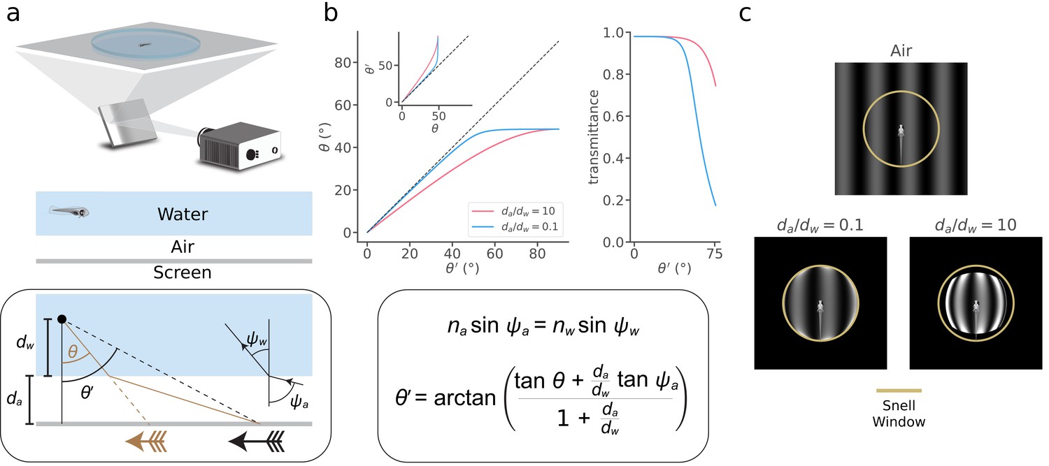
Snell's law describes visual stimulus distortions that occur via air-water interfaces encountered in a typical experiment.

(a) *Top*, In a typical zebrafish neuroscience experiment, an image is presented via projection onto a screen underneath an animal in a water-filled plastic dish. *Middle*, A small layer of air separates the screen from the dish and water. *Bottom box*, This configuration causes the image received at the eye (brown arrow) to be distorted and translated relative to the projected image (black arrow). We can describe this transformation as a relationship between the true position of a projected point ( $θ^{'}$ ) and its apparent position ( $θ$ ), depending on the ratio between the distance from the air-water interface to the screen ( $d_{a}$ ) and the distance from the eye to the air-water interface ( $d_{w}$ ). To solve the transformation, we use Snell’s law (illustrated in inset and panel b), which relates the angle at which a light ray leaves the air-water interface ( $ψ_{w}$ ) to the angle at which it hits the interface ( $ψ_{a}$ ), depending on the refractive indices of the media (air, $n_{a} = 1$ ; water, $n_{w} = 1.333$ ). Note that the effects of the plastic dish are typically minor (Appendix 1). (b) *Top left,* the apparent position of a point ( $θ$ ) as a function of its true position ( $θ^{'}$ ), and its inverse (*inset*), for $d_{a} / d_{w} = 10$ (pink) and $d_{a} / d_{w} = 0.1$ (blue). *Top right*, fraction of light transmitted into the water as a function of $θ^{'}$ for the same two values of $d_{a} / d_{w}$ . *Bottom box*, Using Snell’s law, we derived $θ^{'} (θ)$ (*top left inset*), whose inverse we take numerically to arrive at $θ (θ^{'})$ (*top left*). (c) Simulated distortion of a standard sinusoidal grating. Yellow circle denotes the extent of the Snell window (~97.2° visual angle). The virtual screen is modeled as a 4 × 4 cm square with 250 pixels/cm resolution, and we fixed the total distance between the fish and the virtual screen, $d_{a} + d_{w}$ , to be 1 cm. Note that only a fraction of the screen is apparent when $d_{a} / d_{w}$ is small (*bottom left*), but a distorted view of the full screen appears within the Snell window when $d_{a} / d_{w}$ becomes large (*bottom right*). Contrast axes are matched across panels and saturate to de-emphasize the ring of light at the Snell window, whose magnitude would be attenuated by unmodeled optics in the fish eye (Materials and methods).

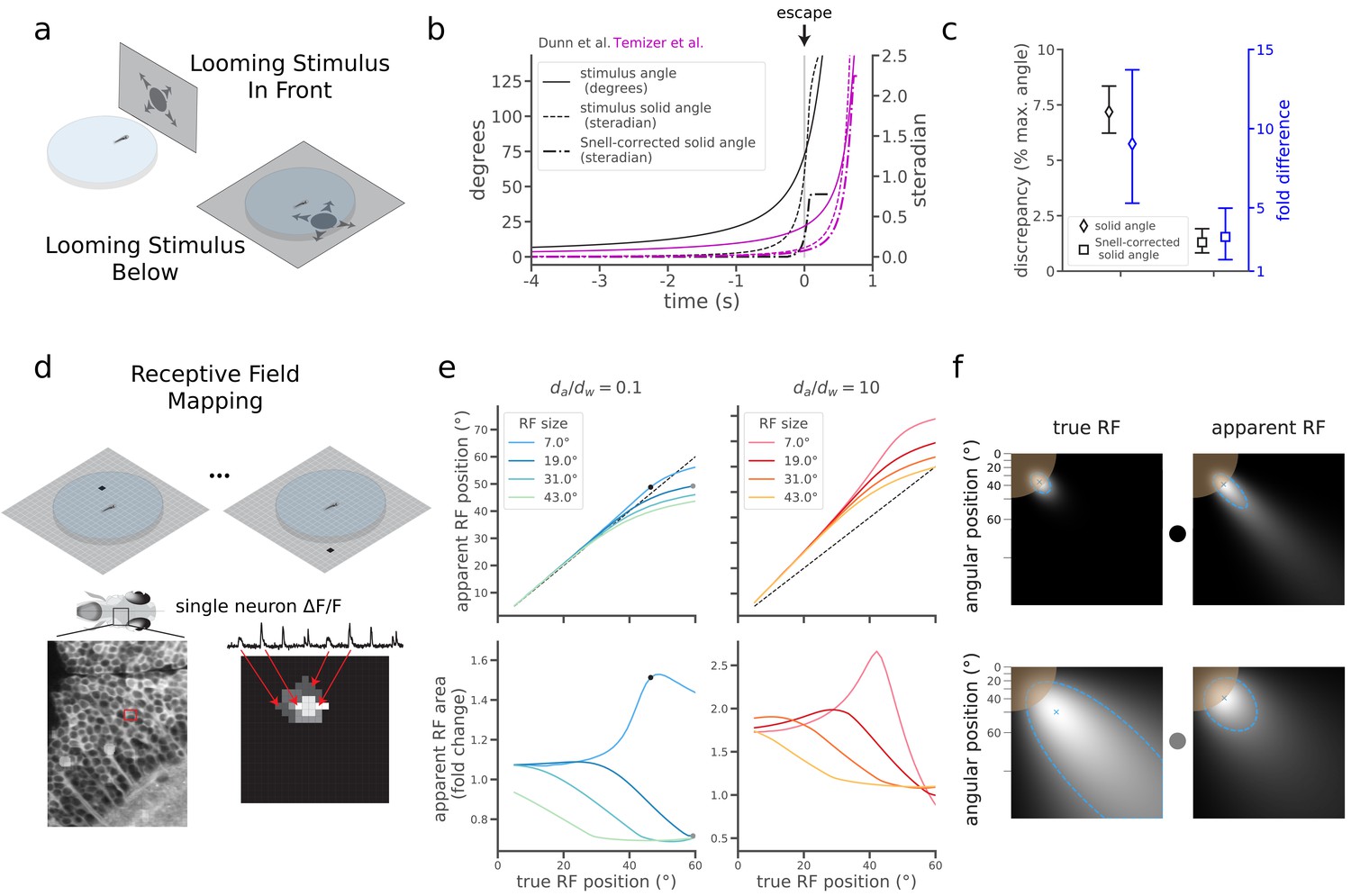
The quantitative merits of correcting for refraction are apparent when comparing two recent studies of visually evoked escape behavior in larval zebrafish. Although Temizer et al. (2015) and Dunn et al., 2016a both found that a critical size of looming stimuli triggered escape behavior, they reported surprisingly different values for the critical angular size (21.7°±4.9° and 72.0°±2.5°, respectively, mean ±95% CI). This naively implies that the critical stimulus of Dunn et al. occupied 9 times the solid angle of Temizer et al. (1.02 [+0.14,–0.11] steradians and 0.11 [+0.06,–0.04] steradians, respectively, mean [95% CI]) (Materials and methods). This large size discrepancy initially raises doubt to the notion that a stimulus size threshold triggers the escape (Hatsopoulos et al., 1995; Gabbiani et al., 1999; Fotowat and Gabbiani, 2011). However, a major difference in experimental design is that Temizer et al. showed stimuli from the front through a curved air-water interface, and Dunn et al. showed stimuli from below through a flat air-water interface (Figure 2a). Correcting the Dunn et al. stimuli with Snell’s law, and again quantifying the size of irregularly shaped stimuli with their solid angle, we found that the fish exhibited escape responses when the stimulus spanned just 0.24 steradians (Figure 2b, Materials and methods, Appendix 1, Figure 2—video 1). The same correction applied to Temizer et al. sets the critical size at 0.08 steradians (Figure 2b, Materials and methods, Appendix 2). This leaves a discrepancy of 0.16 steradians, which is much smaller than the original solid angle discrepancy of 0.91 steradians (Figure 2c, black). Correcting with Snell’s law thus markedly reduced this discrepancy in the literature, shrinking a 9-fold size difference down to 3-fold (Figure 2c, blue). The small remaining difference could indicate an ethologically interesting dependence of behavior on the spatial location of the looming stimulus (Dunn et al., 2016a; Temizer et al., 2015).

Figure 2 with 1 supplement see all

Download asset Open asset

Snell's law corrections reduce discrepancies in the literature and predict effects on receptive field mapping.

(a) In the zebrafish literature, two configurations were used to probe the neural circuitry processing looming stimuli that expand over time. In one, fish were embedded off-center in a curved plastic dish and a screen presented stimuli in front of the animal through the curved interface of the dish (Temizer et al., 2015). In the other, fish were embedded (or swam freely) in a similar dish, but stimuli were presented on a screen below the dish (as in Figure 1a; Dunn et al., 2016a). (b) Plot detailing the changes to the looming expansion time courses after correcting for Snell’s law and converting to solid angle, which more accurately describes the irregular stimulus shapes produced by the optical distortion (Materials and methods). Curves corresponding to Dunn et al. and Temizer et al. are plotted in black and magenta, respectively. (c) Snell’s law corrections reduced the discrepancy between Dunn et al. and Temizer et al. *Black*: Snell’s law corrections decreased the absolute magnitude of the discrepancy (Dunn et al. critical solid angle minus Temizer et al. critical solid angle). We report discrepancies as fractions of the maximal solid angle (4π steradians) to aid intuition for stimulus sizes. *Blue*: Snell’s law corrections also decreased the relative magnitude of the discrepancy (Dunn et al. size divided by Temizer et al. size). (d) In a simple receptive field (RF) mapping experiment, dots appear at different positions on a screen (*Top*), and behavioral or neural responses (*Bottom*) are measured. In the latter case, a map of a single neuron’s RF is constructed by assigning the measured $Δ F / F$ signal to the point on the screen that evoked the $Δ F / F$ response. (e) Snell’s law predicts changes in RF peak positions (*Top*) and RF sizes (*Bottom*). The magnitude of these changes depends on the true RF position (x-axis), true RF size (line color), and $d_{a} / d_{w}$ (warm versus cool colors). True RF positions and sizes correspond to the means and standard deviations of Gaussian receptive fields. The black dots indicate the RFs in *panel f, top*, and the gray dots show the RFs in *panel f*, *bottom*. (f) Illustrations of two simulated "true" RFs and their corresponding measurement distortions predicted using Snell’s law. For simplicity, we show only one quadrant of the screen space, with the fish at the top left corner. The brown circle denotes the extent of the Snell window. As RFs are mapped directly to screen pixels, the axes are nonlinear in terms of angle relative to the fish (top left corner). Each blue "x" denotes the peak position of the RF displayed in each plot. The dashed blue border denotes the half-maximum value of each RF, and the size of the RF is the solid angle within one of these borders.

Accounting for optical distortions will be critical for understanding other fundamental properties of the zebrafish visual system. For example, a basic property of many visual neurons is that they respond strongest to stimuli presented in one specific region of the visual field, termed their receptive field (RF) (Hartline, 1938; Ringach, 2004; Zhang and Arrenberg, 2019). When we simulated the effect of Snell’s law on RF mapping under typical experimental conditions (Figure 2d), we predicted substantial errors in both the position and size of naively measured receptive fields (Figure 2e, Materials and methods). Depending on the properties of the true RF, its position and size could be either over- or under-estimated (Figure 2e–f), with the most drastic errors occurring for small RFs appearing near the edge of the Snell window.

Future experiments could avoid distortions altogether by adjusting experimental hardware. For instance, fish could be immobilized in the center of water-filled spheres (Zhang and Arrenberg, 2019; Dehmelt et al., 2019), or air interfaces could be removed altogether, such as by placing a projection screen inside the water-filled arena. But in practice the former would restrict naturalistic behavior, and the latter would reduce light diffusion by shrinking the refractive index mismatch between the diffuser and transparent medium (water vs. air) that typical light diffusers use to transmit stimuli over a large range of angles. An engineering solution might build diffusive elements into the body of the fish tank (Stowers et al., 2017; Franke et al., 2019). Alternatively, we propose a simple computational solution to account for expected distortions when designing stimuli or analyzing data. Our tool (https://www.github.com/spoonsso/snell_tool/) converts between normal and distorted image representations for the most common zebrafish experiment configuration (Figure 1a), and other geometries could be analyzed similarly. This tool will therefore improve the interpretability and reproducibility of innovative experiments that capitalize on the unique experimental capabilities available in zebrafish neuroscience.

Materials and methods

See Appendix 1 and Appendix 2 for the geometric consequences of Snell’s law at flat and curved interfaces, respectively.

Implications of the Fresnel equations

Request a detailed protocol

Only a portion of the incident light is transmitted into the water to reach the eye. We calculated the fraction of transmitted light according to the Fresnel equations. Assuming the light is unpolarized,

T = 1 - \frac{R_{s} + R_{p}}{2},

where $T$ is the fraction of light transmitted across an air-water interface at incident angle $ψ_{a} = ψ_{a} (θ)$ (See Appendices 1, 2), $ψ_{w} = θ$ is the angle of the refracted light ray in water, and

\begin{array}{ll} R_{s} = & {(\frac{n_{a} \cos ψ_{a} (θ) - n_{w} \cos θ}{n_{a} \cos ψ_{a} (θ) + n_{w} \cos θ})}^{2} \\ R_{p} = & {(\frac{n_{a} \cos θ - n_{w} \cos ψ_{a} (θ)}{n_{a} \cos θ + n_{w} \cos ψ_{a} (θ)})}^{2} \end{array}

are the reflectances for s-polarized (i.e. perpendicular) and p-polarized (i.e. parallel) light, respectively. When including the plastic dish in our simulations, we modified these equations to separately calculate the transmission fractions across the air-plastic and the plastic-water interfaces. We assumed that the full transmission fraction is the product of these two factors, thereby ignoring the possibility of multiple reflections within the plastic.

Illustrating distorted sinusoidal gratings

Request a detailed protocol

For all image simulations in Figure 1c, we neglected the plastic and fixed the total distance between the fish and the virtual screen, $d_{a} + d_{w}$ , to be 1 cm, a typical distance in real-world experiments. The virtual screen was considered to be a 4 × 4 cm square with 250 pixels/cm resolution. Here we assumed that the virtual screen emits light uniformly at all angles, but this assumption is violated by certain displays, and our computational tool allows the user to specify alternate angular emission profiles. To transform images on the virtual screen, we shifted each light ray (i.e. image pixel) according to Snell’s law, scaled its intensity according to the Fresnel equations, and added the intensity value to a bin at the resulting apparent position. This simple model treats the fish eye as a pinhole detector, whereas real photoreceptors blur visual signals on a spatial scale determined by their receptive field. Consequently, our simulation compresses a large amount of light onto the overly thin border of the Snell window, and we saturated the grayscale color axes in Figure 1c to avoid this visually distracting artifact.

To make the image as realistic as possible, we mimicked real projector conditions using gamma-encoded gratings with spatial frequency 1 cycle / cm, such that

{[x (t)]}^{1 / 2.2} = \sin t

with $x (t)$ ranging from 1.0 to 500.0 lux, a standard range of physical illuminance for a lab projector. The exponent on the left represents a typical display gamma encoding with gamma = 2.2. To reduce moiré artifacts arising from ray tracing, we used a combination of ray supersampling (averaging the rays emanating from 16 sub-pixels for each virtual screen pixel) and stochastic sampling (the position of each ray was randomly jittered between -1 and 1 sub-pixels from its native position) (Dippé and Wold, 1985). In Figure 1c, we display the result of these operations followed by a gamma compression to mimic the perceptual encoding of the presented stimulus.

Corrections to looming visual stimuli

Request a detailed protocol

We approximated the geometric parameters from Dunn et al. (2016a) (flat air-water interface, d_a = 0.5 mm, d_w = 3 mm, d_p = 1 mm, stimulus offset from the fish by 10 mm along the screen) and Temizer et al., 2015 (curved air-water interface, d_a = 8 mm, d_w = 2 mm, d_p = 1 mm, r = 17.5 mm, stimulus centered) to create Snell-transformed images of circular stimuli with sizes growing over time (Figure 2a–c). We used a refractive index of n_p = 1.55 for the polystyrene plastic. While Dunn et al. collected data from freely swimming fish, the height of the water was kept at approximately 5 mm, and 3 mm reflects a typical swim depth. Since freely swimming zebrafish can adjust their depth in water, it’s an approximation to treat d_w as constant.

We quantified the size of each transformed stimulus with its solid angle, the surface area of the stimulus shape projected onto the unit sphere. To calculate the solid angle for Temizer et al., we used the formula for a spherical cap, $A = 2 π (1 - \cos θ)$ , where $A$ is the solid angle and $2 θ$ is the apex angle. To calculate the solid angle for Dunn et al., in which stimuli were not spherical caps, we first represented stimulus border pixels in a spherical coordinate system locating the fish at the origin. The radial coordinate does not affect the solid angle, so we described each border pixel by two angles: the latitude, α, and longitude, $β$ . To calculate the area, we used an equal-area sinusoidal (Mercator) projection given by

(x, y) = (β \cos α, α),

which projects an arbitrary shape on the surface of a sphere onto the Cartesian plane. While distances and shapes are not preserved in this projection, area as a fraction of the sphere’s surface area is maintained. Thus, we could calculate the solid area of the stimulus in this projection by finding the area of the projected 2D polygon. To calculate the absolute and relative discrepancy 95% confidence intervals in Figure 2c, we used error propagation formulae for the difference and division of two distributions, respectively.

Receptive field mapping

Request a detailed protocol

We simulated receptive field (RF) mapping experiments by tracing light paths from single pixels on a virtual screen to the fish (Figure 2d-f). We modeled a neuron’s RF as a Gaussian function on the sphere, defined the “true RF” to be the pixel-wise response pattern that would occur in the absence of the air-water interface, and defined the “apparent RF” as the pixel-wise response pattern that would be induced with light that bends according to Snell’s law at an air-water interface. More precisely, we modeled the neural response to pixel activation at position $x$ as

F (x) = T (ψ_{a} (x)) P (ρ (x, μ_{R F}), σ_{R F}^{2}),

where $T (ψ_{a} (x))$ is the fraction of light transmitted (Fresnel equations), $μ_{R F}$ and $σ_{R F}$ are the mean and standard deviation of the Gaussian RF, $ρ (x, μ_{R F})$ is the distance along a great circle from the center of the RF to the pixel’s projected retinal location, and $P (ρ, σ_{R F}^{2}) = e^{- ρ^{2} / (2 σ_{R F}^{2})}$ is the Gaussian RF shape. We calculated the great circle distance between points on the sphere as

\cos ρ (x, μ_{R F}) = \sin α_{R F} \sin α_{x} + \cos α_{R F} \cos α_{x} \cos (β_{x} - β_{R F}),

where $(α_{R F}, β_{R F})$ are the latitude and longitude coordinate of the RF center, and $(α_{x}, β_{x})$ are the latitude and longitude coordinates of the projected pixel location. We quantified the position of the RF as the maximum of $F (x)$ , converted to an angular coordinate along the screen. We quantified RF area as the solid angle of the shape formed by thresholding $F (x)$ at half its maximal value.

Computational tool for simulating and correcting optical distortions

Request a detailed protocol

With this paper, we provide a computation tool for visualizing and correcting distortions (https://github.com/spoonsso/snell_tool/). The tool is written in Python and uses standard image processing libraries. The tool can be launched virtually over the web, without any need to install new software, using the MyBinder link in the README file hosted on the github repository. The source code can also be downloaded and run on the user’s local machine.

The uses and parameters of the tool are described in detail in an example notebook in the repository (snell_example.ipynb). In brief, the tool is implemented only for flat interfaces with the assumptions described in Appendix 1, and it can model distortions through three media (i.e. with a plastic interface between air and water). It can also model displays that emit light with non-uniform angular profiles. Key customizable parameters include the screen size, screen resolution, screen distance, media thicknesses, media refractive indices, and gamma encoding. As described in Illustrating distorted sinusoidal gratings, the tool uses a combination of ray super-sampling and stochastic sampling to reduce moiré artifacts arising from ray tracing.

The Python notebook illustrates two primary use cases of the tool, though the tool’s library is flexible enough to be adopted for other tasks. First, it allows the user to input an image to see its distorted form under the assumptions of the model. Thus, it recreates Figure 1c, but for any arbitrary grayscale stimulus, and for a range of user-specified experimental configurations. Second, it allows the user to input an undistorted target image, and the tool inverts the distortion process to suggest an image that could be displayed during an experiment to approximately produce the target from the point of view of the fish. In the tool’s example notebook, we demonstrate this inversion process using a checkered ball stimulus. Importantly, note that some stimuli will be physically impossible to correct (e.g. undistorted image content cannot be delivered outside the Snell window).

Appendix 1

Implications of Snell’s law at a flat interface

For this and all subsequent analyses, we treat the fish as a pinhole detector. Here we derive $θ^{'} (θ)$ with the aid of Appendix 1—figure 1. Note that this derivation includes optical effects from the plastic dish, but these effects will be relatively minor. To begin, we summarize the basic trigonometry of the problem. The true angular position of the stimulus is given by

\tan θ' = \frac{{d'}_{w} + {d'}_{p} + {d'}_{a}}{d_{w} + d_{p} + d_{a}},

where $d_{w}$ is the normal distance between the fish and the water-plastic interface, $d_{p}$ is the normal distance between the water-plastic and plastic-air interfaces, $d_{a}$ is the normal distance between the air interface and the screen (interface and screen assumed to be parallel), ${d'}_{w}$ is the parallel distance traveled by the light ray in the water, ${d'}_{p}$ is the parallel distance traveled by the light ray in the plastic, and ${d'}_{a}$ is the parallel distance traveled by the light ray in air. Each parallel distance is related to the corresponding normal distance by simple trigonometry. The apparent angular location of the stimulus satisfies

d_{w}^{'} = d_{w} \tan θ,

and the incident light angle satisfies

\begin{array}{ll} d_{a}^{'} = & d_{a} \tan ψ_{a}, \\ d_{p}^{'} = & d_{p} \tan ψ_{p}, \end{array}

thereby leading to

θ^{'} = \tan^{- 1} (\frac{d_{w} \tan θ + d_{p} \tan ψ_{p} + d_{a} \tan ψ_{a}}{d_{w} + d_{p} + d_{a}}) .

We can next use Snell’s law to reduce the number of angular variables. In particular,

ψ_{p} = \sin^{- 1} (\frac{n_{w} \sin ψ_{w}}{n_{p}}) = \sin^{- 1} (\frac{n_{w} \sin θ}{n_{p}})

and

ψ_{a} = \sin^{- 1} (\frac{n_{p} \sin ψ_{p}}{n_{a}}) = \sin^{- 1} (\frac{n_{p} \sin (\sin^{- 1} (\frac{n_{w} \sin θ}{n_{p}}))}{n_{a}}) = \sin^{- 1} (\frac{n_{w} \sin θ}{n_{a}})

together imply that

θ^{'} (θ) = \tan^{- 1} (\frac{d_{w} \tan θ + d_{p} \tan (\sin^{- 1} (\frac{n_{w} \sin θ}{n_{p}})) + d_{a} \tan (\sin^{- 1} (\frac{n_{w} \sin θ}{n_{a}}))}{d_{w} + d_{p} + d_{a}}) .

The role of plastic in this equation is typically minimal. To see this, first note that $n_{w} \approx 1.333 < n_{p} \approx 1.55$ , which implies that $\frac{n_{w} \sin θ}{n_{p}} < 1$ . This implies that the Snell window is determined by $1 = \frac{n_{w} \sin θ}{n_{a}}$ , and the properties of the high-index plastic dishes have no effect on the size of the Snell window. The plastic can cause distortions within the Snell window, but these effects were small for all experimental arenas analyzed in this paper, as we empirically found that none of our results qualitatively depended upon the plastic. We therefore chose to highlight the critical impact of the air-water interface by assuming that $d_{p} = 0$ in the main text’s conceptual discussion. We nevertheless included nonzero values of $d_{p}$ in our computational tool so that users can account for the quantitative effects of the plastic dish. We also included the effects of plastic when quantitatively correcting previously published results. Because analytically inverting $θ^{'} (θ)$ is non-trivial, we noted from the graph of $θ^{'} (θ)$ that the inverse function exists and calculated $θ (θ')$ with a numerical look-up table (e.g. Figure 1b).

Appendix 1—figure 1

Download asset Open asset

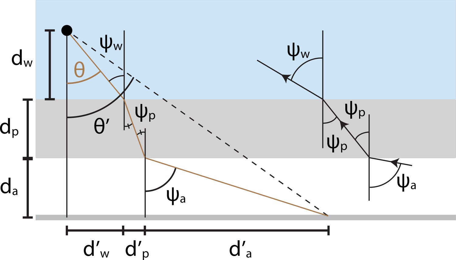
Illustration of mathematical variables used to analyze optical distortions in arena geometries where flat air-plastic and plastic-water interfaces separate the fish from the projection screen.

The brown line denotes the trajectory of a light ray traveling from the screen to the fish. We quantify the image transformation by relating the true angular position of each projected point ( $θ^{'}$ ) to its apparent position ( $θ$ ). The derivation involves several distances (e.g. $d_{w}$ ) that summarize the ray’s trajectory through air (white region), plastic (gray region), and water (blue region). Refraction angles ( $ψ_{a}, ψ_{p}, ψ_{w}$ ) describe the bending of light at each interface.

Appendix 2

Implications of Snell’s law at a curved interface

When the fish is mounted off-center (Appendix 2—figure 1a) in a circular dish (brown dot), rays pass through a curved interface and are refracted at tangent lines (brown line). We begin by using Snell’s law and basic trigonometry to relate each refraction angle to $θ$ . Let $d_{a}$ denote the distance in air between the edge of the plastic dish and the screen, $d_{p}$ denote the thickness of the plastic dish, $d_{w}$ denote the distance in water between the fish and the edge of the tank nearest the screen, and $r$ denote the radius of the dish (excluding the plastic). We assume that $d_{w} \leq r$ and the screen is perpendicular to the line between the fish and the center of the dish. Cases where the fish is behind the dish’s center or the screen is angled can be analyzed similarly. Starting at the fish and moving outwards, we first apply the law of sines to the gray triangle to find

\frac{\sin (ψ_{w})}{{r - d}_{w}} = \frac{\sin (π - θ)}{r} ⟹ \sin (ψ_{w} (θ)) = \frac{{r - d}_{w}}{r} \sin (θ),

where we’ve used the identity $\sin (π - x) = \sin (x)$ . It will be useful for later to note that this triangle also implies that $γ = π - (ψ_{w} + π - θ) = θ - ψ_{w}$ . Snell’s law at the plastic-water interface implies,

n_{p} \sin (ψ_{p}) = n_{w} \sin (ψ_{w}) ⟹ \sin (ψ_{p} (θ)) = \frac{n_{w}}{n_{p}} \sin (ψ_{w}) = \frac{n_{w}}{n_{p}} \frac{r - d_{w}}{r} \sin (θ) .

We next relate the two plastic refraction angles to each other by applying the law of sines to the orange triangle and find

\frac{\sin (ψ_{p}^{'})}{r} = \frac{\sin (π - ψ_{p})}{r + d_{p}} ⟹ \sin (ψ_{p}^{'} (θ)) = \frac{r}{r + d_{p}} \sin (ψ_{p}) = \frac{n_{w}}{n_{p}} \frac{r - d_{w}}{r + d_{p}} \sin (θ) .

Finally, we determine the dependence of $ψ_{a}$ on $θ$ from Snell’s law applied to the air-plastic interface,

n_{a} \sin (ψ_{a}) = n_{p} \sin (ψ_{p}^{'}) ⟹ \sin (ψ_{a} (θ)) = \frac{n_{p}}{n_{a}} \sin (ψ_{p}^{'}) = \frac{n_{w}}{n_{a}} \frac{r - {d mi>}_{w}}{r + d_{p}} \sin (θ) .

With these formulae in hand, we now proceed to the main goal of deriving an expression for $θ^{'} (θ)$ . Since we’ve already extracted everything from Snell’s law, all that remains is basic trigonometry, which we illustrate in Appendix 2—figure 1b. First note that applying the definition of the tangent function to the blue triangle implies that

θ^{'} (θ) = \tan^{- 1} (\frac{s (θ) + s' (θ)}{d_{a} + d_{p} + d_{w}}) .

It thus suffices to determine expressions for $s (θ)$ and $s' (θ)$ . Consider first $s' (θ)$ . The large red triangle implies

s^{'} (θ) = (r + d_{p} + d_{a}) \tan (α (θ)) .

Rewriting $α$ in terms of the other two angles in the $α β ψ_{p}^{'}$ triangle gives $α = π - β - ψ_{p}^{'}$ . Rewriting $β$ in terms of the other two angles in the $β {γ ψ}_{p}^{}$ triangle gives $β = π - (γ + ψ_{p}) = π - θ + ψ_{w} - ψ_{p}$ . Putting these pieces together, we thus find

α (θ) = θ - ψ_{p}^{'} (θ) + ψ_{p} (θ) - ψ_{w} (θ) .

Next consider $s (θ)$ . Applying the law of sines to the green triangle, we find

\frac{\sin (ψ_{a})}{s} = \frac{\sin (ω)}{a} \Rightarrow s (θ) = \frac{a (θ) \sin (ψ_{a} (θ))}{\sin (ω (θ))} .

Rewriting $ω$ in terms of the other two angles in the green triangle, $ω = π - (ψ_{a} + π - φ) = φ - ψ_{a}$ , and rewriting $φ$ in terms of the other angles in the red triangle, $φ = π - (α + \frac{π}{2}) = \frac{π}{2} - α$ , we find

ω (θ) = \frac{π}{2} - θ - ψ_{a} (θ) + ψ_{p}^{'} (θ) - ψ_{p} (θ) + ψ_{w} (θ) .

Finally, we find the dependence of $a$ on $θ$ from the red triangle using the definition of the cosine function

\cos (α) = \frac{r + d_{p} + d_{a}}{r + d_{p} + a} ⟹ a (θ) = \frac{r + d_{p} + d_{a}}{\cos (α (θ))} - r - d_{p} .

Since we’ve written $α$ , $a$ , $ω$ , and the refraction angles as functions of $θ$ , we’ve fully specified $s (θ)$ , $s' (θ)$ , and thus $θ^{'} (θ)$ . As with the flat interface, we calculated $θ (θ')$ using a numerical look-up table.

Appendix 2—figure 1

Download asset Open asset

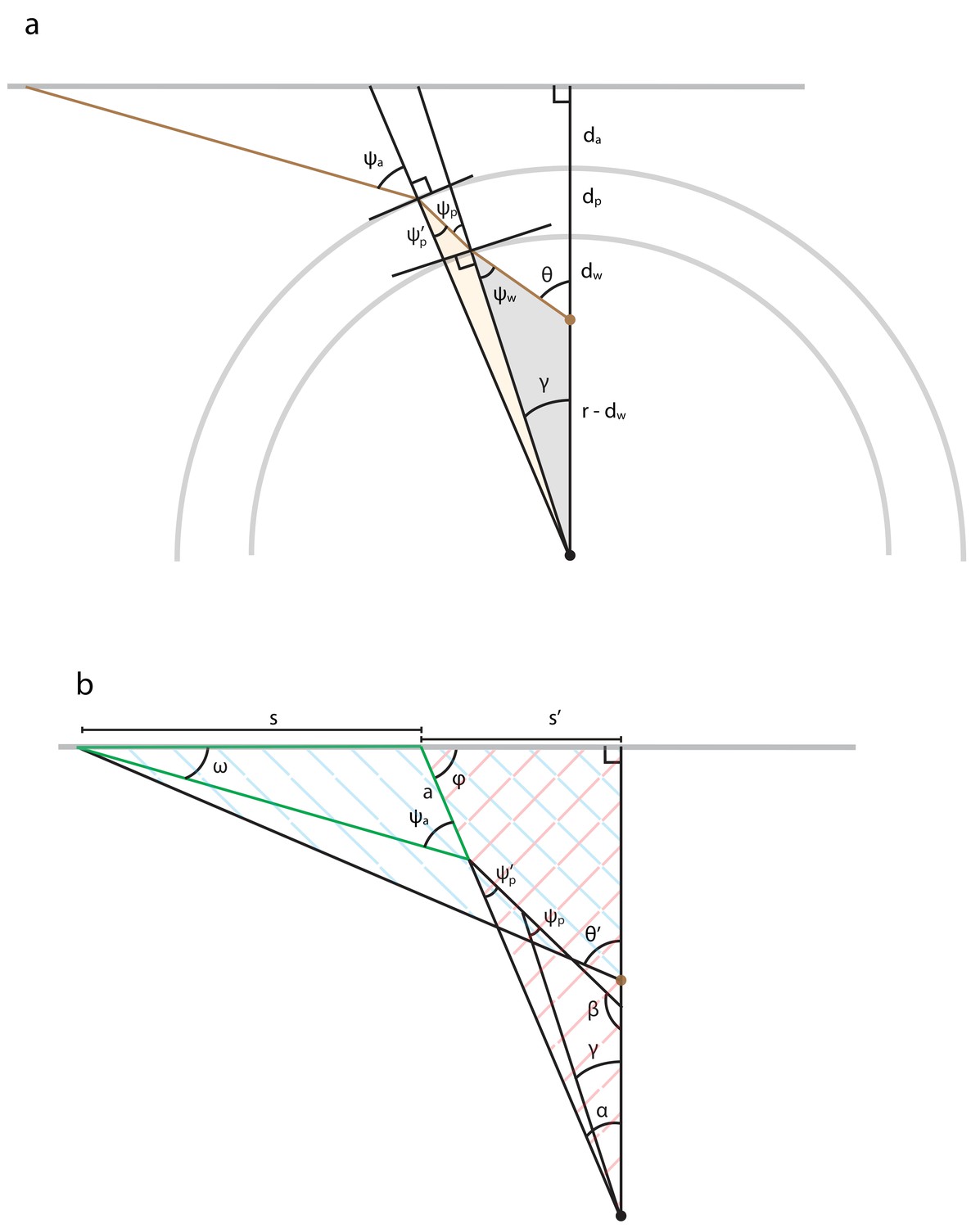
Illustration of mathematical variables used to analyze optical refraction at curved interfaces.

(a) We assume that the interfaces are circular, that the fish is mounted off-center (brown dot), and that the screen and fish are at the same elevation. We neglect distortions that could result from the flat vertical interface running parallel to the longitudinal axis of the cylindrical dish. We denote the radius of the arena’s water-filled compartment as $r$ . The derivation additionally involves several distances that summarize the placement of the fish in the dish ( $d_{w}$ ), the thickness of the plastic ( $d_{p}$ ), and the distance separating the dish from the screen ( $d_{a}$ ). Refraction angles ( $ψ_{a}, ψ_{p}^{'}, ψ_{p}, ψ_{w}$ ) of the light ray (brown line) are relative to each interface’s normal vector and describe the bending of light. Each shaded region highlights a triangle whose trigonometry is helpful for relating the refraction angles to the apparent angular position of a light source ( $θ$ ). (b) Illustration of mathematical variables used to trigonometrically relate the true angular position of each projected point ( $θ^{'}$ ) to its apparent position ( $θ$ ), assuming the same arena geometry as panel a. The derivation utilizes most triangles shown, several of which are cross-hatched or outlined to direct the reader’s eye.

Data availability

No data were collected for this theoretical manuscript.

References

1. Ahrens MB
2. Li JM
3. Orger MB
4. Robson DN
5. Schier AF
6. Engert F
7. Portugues R
(2012) Brain-wide neuronal dynamics during motor adaptation in zebrafish
Nature 485:471–477.
https://doi.org/10.1038/nature11057
- PubMed
- Google Scholar
1. Ahrens MB
2. Orger MB
3. Robson DN
4. Li JM
5. Keller PJ
(2013) Whole-brain functional imaging at cellular resolution using light-sheet microscopy
Nature Methods 10:413–420.
https://doi.org/10.1038/nmeth.2434
- PubMed
- Google Scholar
Preprint
1. Dehmelt FA
2. Meier R
3. Hinz J
4. Yoshimatsu T
5. Simacek CA
6. Wang K
7. Baden T
8. Arrenberg AB
(2019) Spherical arena reveals optokinetic response tuning to stimulus location size and frequency across entire visual field of larval zebrafish
bioRxiv.
https://doi.org/10.1101/754408
- Google Scholar
1. Dippé MAZ
2. Wold EH
(1985) Antialiasing through stochastic sampling
ACM SIGGRAPH Computer Graphics 19:69–78.
https://doi.org/10.1145/325165.325182
- Google Scholar
1. Dunn TW
2. Gebhardt C
3. Naumann EA
4. Riegler C
5. Ahrens MB
6. Engert F
7. Del Bene F
(2016a) Neural circuits underlying visually evoked escapes in larval zebrafish
Neuron 89:613–628.
https://doi.org/10.1016/j.neuron.2015.12.021
- PubMed
- Google Scholar
1. Dunn TW
2. Mu Y
3. Narayan S
4. Randlett O
5. Naumann EA
6. Yang CT
7. Schier AF
8. Freeman J
9. Engert F
10. Ahrens MB
(2016b) Brain-wide mapping of neural activity controlling zebrafish exploratory locomotion
eLife 5:e12741.
https://doi.org/10.7554/eLife.12741
- PubMed
- Google Scholar
1. Fotowat H
2. Gabbiani F
(2011) Collision detection as a model for sensory-motor integration
Annual Review of Neuroscience 34:1–19.
https://doi.org/10.1146/annurev-neuro-061010-113632
- PubMed
- Google Scholar
1. Franke K
2. Maia Chagas A
3. Zhao Z
4. Zimmermann MJ
5. Bartel P
6. Qiu Y
7. Szatko KP
8. Baden T
9. Euler T
(2019) An arbitrary-spectrum spatial visual stimulator for vision research
eLife 8:e48779.
https://doi.org/10.7554/eLife.48779
- PubMed
- Google Scholar
(1999) Computation of object approach by a wide-field, motion-sensitive neuron
The Journal of Neuroscience 19:1122–1141.
https://doi.org/10.1523/JNEUROSCI.19-03-01122.1999
- PubMed
- Google Scholar
1. Hartline HK
(1938)
The response of single optic nerve fibers

The American Journal of Physiology 121:400–415.
- Google Scholar
(1995) Elementary computation of object approach by wide-field visual neuron
Science 270:1000–1003.
https://doi.org/10.1126/science.270.5238.1000
- PubMed
- Google Scholar
Book
1. Hecht E
(2016)
Optics (Fifth Edition)

Pearson Education.
- Google Scholar
1. Kim DH
2. Kim J
3. Marques JC
4. Grama A
5. Hildebrand DGC
6. Gu W
7. Li JM
8. Robson DN
(2017) Pan-neuronal calcium imaging with cellular resolution in freely swimming zebrafish
Nature Methods 14:1107–1114.
https://doi.org/10.1038/nmeth.4429
- PubMed
- Google Scholar
(2016) From whole-brain data to functional circuit models: the zebrafish optomotor response
Cell 167:947–960.
https://doi.org/10.1016/j.cell.2016.10.019
- PubMed
- Google Scholar
(2014) Whole-brain activity maps reveal stereotyped, distributed networks for visuomotor behavior
Neuron 81:1328–1343.
https://doi.org/10.1016/j.neuron.2014.01.019
- PubMed
- Google Scholar
1. Prevedel R
2. Yoon YG
3. Hoffmann M
4. Pak N
5. Wetzstein G
6. Kato S
7. Schrödel T
8. Raskar R
9. Zimmer M
10. Boyden ES
11. Vaziri A
(2014) Simultaneous whole-animal 3D imaging of neuronal activity using light-field microscopy
Nature Methods 11:727–730.
https://doi.org/10.1038/nmeth.2964
- PubMed
- Google Scholar
1. Ringach DL
(2004) Mapping receptive fields in primary visual cortex
The Journal of Physiology 558:717–728.
https://doi.org/10.1113/jphysiol.2004.065771
- PubMed
- Google Scholar
1. Sajovic P
2. Levinthal C
(1983) Inhibitory mechanism in zebrafish optic tectum: visual response properties of tectal cells altered by picrotoxin and bicuculline
Brain Research 271:227–240.
https://doi.org/10.1016/0006-8993(83)90285-8
- PubMed
- Google Scholar
(2017) Virtual reality for freely moving animals
Nature Methods 14:995–1002.
https://doi.org/10.1038/nmeth.4399
- PubMed
- Google Scholar
(2015) A visual pathway for looming-evoked escape in larval zebrafish
Current Biology 25:1823–1834.
https://doi.org/10.1016/j.cub.2015.06.002
- PubMed
- Google Scholar
1. Vladimirov N
2. Mu Y
3. Kawashima T
4. Bennett DV
5. Yang CT
6. Looger LL
7. Keller PJ
8. Freeman J
9. Ahrens MB
(2014) Light-sheet functional imaging in fictively behaving zebrafish
Nature Methods 11:883–884.
https://doi.org/10.1038/nmeth.3040
- PubMed
- Google Scholar
1. Vladimirov N
2. Wang C
3. Höckendorf B
4. Pujala A
5. Tanimoto M
6. Mu Y
7. Yang CT
8. Wittenbach JD
9. Freeman J
10. Preibisch S
11. Koyama M
12. Keller PJ
13. Ahrens MB
(2018) Brain-wide circuit interrogation at the cellular level guided by online analysis of neuronal function
Nature Methods 15:1117–1125.
https://doi.org/10.1038/s41592-018-0221-x
- PubMed
- Google Scholar
1. Zhang Y
2. Arrenberg AB
(2019) High throughput, rapid receptive field estimation for global motion sensitive neurons using a contiguous motion noise stimulus
Journal of Neuroscience Methods 326:108366.
https://doi.org/10.1016/j.jneumeth.2019.108366
- PubMed
- Google Scholar

Decision letter

Claire Wyart

Reviewing Editor; Institut du Cerveau et la Moelle épinière, Hôpital Pitié-Salpêtrière, Sorbonne Universités, UPMC Univ Paris 06, Inserm, CNRS, France
Didier YR Stainier

Senior Editor; Max Planck Institute for Heart and Lung Research, Germany
André Maia Chagas

Reviewer; University of Tübingen, Germany

In the interests of transparency, eLife publishes the most substantive revision requests and the accompanying author responses.

Thank you for submitting your article "Correcting for physical distortions in visual stimuli improves reproducibility in zebrafish neuroscience." for consideration by eLife. Your article has been reviewed by three peer reviewers, and the evaluation has been overseen by a Reviewing Editor and Didier Stainier as the Senior Editor. The following individual involved in review of your submission has agreed to reveal their identity: Andre Maia Chagas (Reviewer #3).

The reviewers have discussed the reviews with one another and the Reviewing Editor has drafted this decision to help you prepare a revised submission.

Summary:

The three reviewers agree that the study is of general interest and will help future studies on visual integration in zebrafish properly design their setups. Precisions and corrections are listed below. Please address all points raised and improve clarity of figures, check legends of supplementary videos.

Reviewer #1:

In this manuscript, the authors describe how to correct for distortions of the light path in vision experiments in aquatic animals. They first discuss and illustrate relevant physical laws and then showcase how distortions associated with suboptimal stimulus configurations could have affected two recent studies on looming stimuli in zebrafish. The impact of their manuscript can be subdivided into the following four points.

1) They raise awareness about stimulus stretching, compression and attenuation occurring in aquatic stimulus setups, which have oftentimes been ignored in zebrafish vision research. This will certainly be of high interest for the growing community of scientists working with aquatic animals, especially zebrafish.

2) The authors show that a critical parameter (d_a/d_w) determines how the physical laws (Fresnel equations, Snell's law) will affect the stimulus appearance in one of the frequently used recording configurations: the apparent position of a stimulus is shown to depend on the ratio of the water column length and the free-air distance between display and water container (d_a/d_w). While the physical laws are no news, the provided equation can be useful for scientists working with such a recording configuration.

3) They calculate, how stimuli have likely been distorted in two recent publications. This is a very helpful type of analysis that can potentially correct/explain observed differences in studies. The authors state that in the original publications the critical stimulus sizes were reported as 21.7° and 72.0° (difference: factor 3.3), and after their correction, the stimulus sizes were 0.6% and 1.9% (of 4π steradians, difference: factor 3.2). If I understand the authors correctly, the authors take the small absolute difference of 1.9% and 0.6% ( = 1.3%) as evidence for a better match after optical correction, because the absolute difference (14%) in the original studies before correction (72° – 21.7°=50.3° ~ = 14% of 360 degrees) had been much bigger. However, I don't agree that this is the best way to compare the results. The relative difference is about a factor of 3 in both cases, so not much different after correction. That being said, it is of course nonetheless very useful to perform these distortion calculations as they can be used to report the stimulus characteristics from the animal's perspective, which is what matters.

4) A programming tool is provided to help scientists calculate the distortions in their setups. It would be helpful if the functionality (inputs, outputs, available configurations) were described in more detail in the manuscript. The tool can be used for the experimental setup in Figure 1A, but for other configurations, users likely need to adapt it or use other software for ray tracing.

In summary, I think that the topic of the manuscript will be of interest to the community of aquatic vision researchers. The presented results and discussion present a rather incremental scientific advance, but are timely for zebrafish vision researchers.

Reviewer #2:

In this study, Dunn and Fitzgerald evaluate the effects of refractive index mismatches and consequent visual distortions upon zebrafish visual neuroscience experiments. They show that refraction at water-air interfaces causes distortions and translations to visual stimuli that, if ignored, will lead to erroneous conclusions about receptive field properties of visual neurons and visuomotor relationships. They show that accounting for Snell's law explains a large part of the apparent discrepancy between the critical angular sizes reported in two studies of looming-evoked escape behavior. The authors also provide a software tool to simulate the effects of refraction on visual stimuli.

Overall, this paper and the associated software will be of considerable value to the growing community of researchers investigating the larval zebrafish visual system. By highlighting an issue that has hitherto largely been ignored and providing means to improve experimental design and interpretation, the paper should enhance the quality and reproducibility of experiments in this important neuroscience model.

I have two main comments:

1) The authors do not appear to have considered the angular intensity profiles of the screens used to present visual cues. However, this will influence the most eccentric location at which an image feature (pixel) is visible to the fish as well as the observed intensity distribution. Moreover, the types of screens used in different studies vary. For example, Dunn et al. used a diffusive screen (for back projection) which will have some scattering characteristic – how was this modeled? Temizer et al. used an OLED screen where individual pixels have a (likely more limited) angular emission profile. This will determine the maximal theta' from which a ray can be emitted that will reach the fish, causing clipping at eccentric locations an affecting the size and amplitude profile of receptive fields. Can the authors incorporate the angular intensity profile of the presentation screen into their modeling (tool)?

2) It was not clear to me why the maximum image size is assumed to be 360° or 4π steradians. In the Dunn and Temizer papers, I assume angular size is computed according to a simple 2D model where one eye views a directly approaching orthogonal object.

In this case, the largest angular size subtended at the eye is 180° (at impact). However, the largest image size cast on the retina of a real eye will be limited by the visual field of that eye (and thus occur prior to impact). Similarly, for the analysis of solid angle, the authors compute percentages assuming a maximal size of 4π, which is clearly not biologically plausible. I would find it more useful if image sizes were given as a proportion of the (monocular) visual field. What is this estimated to be?

Reviewer #3:

I would like to start by thanking the authors for putting this paper together, as it is well written and definitely an asset for experimenters working with aquatic species, or in general for any other researchers that have visual stimuli that need to go through different media before reaching the animal/subject. I'm surprised that this issue hasn't been raised before, but glad to see that this is done here. I also enjoy the fact that they made a repository with more details on the tool they are proposing as a solution to the issue reported here, also that you can reproduce the paper's figures using this repository.

Here are some comments I hope will make the paper even more enjoyable:

1) Would it be possible for the authors to setup their repository to work with "My Binder" (https://mybinder.org/), so that readers who are not using/familiar with python could still use their notebook?

2) In the second paragraph of the main text the authors state that in traditional experimental setups for zebrafish, due to Snell's law, stimuli that are distant appear to the fish at the asymptotic value of ~48.6°, and that this would lead to a "Snell window" of 97.2°. I think this leads to some interesting questions:

2.1) In this setup configuration, the Snell window is covering what area of the bottom of the Petri dish? It would be nice to see visually represented what is the projection size of the window as size of the dish, since:

2.1.1) If the window is only covering part of the dish, the animals are freely moving, and the correction algorithm is used, this would mean that as the animals move, they could go past the edge of the window and be in a region where the stimulus is not present?

2.1.2) It would be nice to know how big the window projection is in relation to the animal's visual space, and how the distance between the petri dish and the projection window change this

3) The authors also mention that having water instead of air in the space between the petri-dish and the projection could be used as an alternative solution to the problem (main text, last paragraph), with the shortcoming of having a reduced transmission of stimuli in large angles. I wonder what these large angles would be? Would this be something easy to calculate? I wonder about this, since Franke et al. (https://elifesciences.org/articles/48779), show a "fish cinema" system where a lot of the fish's field of view is covered (while projecting directly at a screen which was the water container wall – so no air or water interface before the projected image)

4) One thing that I didn't see mentioned in the paper is chromatic aberration. Given the fact that stimuli are travelling through 3 different media at least, one could expect that different wavelengths will be projected slightly misaligned when compared to one another, especially considering the wide chromatic range present in Zebrafish vision? I wonder if it would be easy to incorporate these calculations in the tools they are describing, and most importantly, how could this affect the calculation of receptive fields, considering the misaligned patches of different wavelengths could directly influence some of these receptive fields?

I'm happy to clarify any points that might be unclear, or provide further arguments for the above mentioned points.

[Editors' note: further revisions were suggested prior to acceptance, as described below.]

Thank you for resubmitting your work entitled "Correcting for physical distortions in visual stimuli improves reproducibility in zebrafish neuroscience." for further consideration by eLife. Your revised article has been evaluated by Didier Stainier as the Senior Editor, and a Reviewing Editor.

The manuscript has been improved but there are some remaining issues that need to be addressed before acceptance, as outlined below:

The reviewers have addressed most of the comments from the three reviewers satisfactorily. The authors now include a description of the relative differences of solid angles between the two studies, which is good. However, the presentation is still somewhat confusing for readers, because the comparison of fractional apex angles and fractional solid angles introduces a huge difference simply due to the fact of switching from a one-dimensional to a two-dimensional/squared parameter (the solid angle is proportional to the surface area of the sphere). Thus, the effect of the optical correction is partially masked by the effect of this parameter conversion, and the current text fails to make this transparent and resolve it for the reader.

1) Without optical correction, the absolute difference of 70.3° and 21.7° corresponds to solid angles of 1.15 sr and 0.112 sr, which is a 10-fold relative difference [according to the equation Ω=2π1-cosθ; Ω corresponds to the solid angle, 2θ to the apex, see https://en.wikipedia.org/wiki/Solid_angle]. After optical correction, the relative difference is reduced to 3-fold (0.24 sr vs. 0.08 sr).

Our suggestion is to present results in the main text and in Figure 2C in relative steradian terms. The authors could state that the initial 10-fold difference in covered stimulus area (between the two studies) was surprising, but that after optical correction, this difference is reduced markedly (by a factor of 3).

The remaining 3-fold difference could potentially be explained by a dependence of behavior on the spatial stimulus location (as the authors already write). If the authors structure the paragraph like this, they could then also delete the following sentence, which they need in their current version to present results accurately, but which can be confusing and anticlimactic for readers and the story: "These corrections did not eliminate the discrepancy in relative terms, as Dunn et al. still found a critical size that was approximately three times as large as Temizer et al.".

2) We are not convinced that a 50.3° difference is "far more striking" than a similar relative difference at small stimulus sizes (as the authors state in their point-by-point response). Sensory systems typically encode stimulus magnitudes in logarithmic terms (Weber-Fechner law).

According to the logic used by the authors, a difference of 50.3° is striking irrespective of the base stimulus size. I think they would agree though, that two stimuli, 360° and 310.7° in size, are not very different. This is why the description of differences in relative terms is important, which the authors have now included in their revision.

https://doi.org/10.7554/eLife.53684.sa1

Author response

Reviewer #1:

[…] 1) They calculate, how stimuli have likely been distorted in two recent publications. This is a very helpful type of analysis that can potentially correct/explain observed differences in studies. The authors state that in the original publications the critical stimulus sizes were reported as 21.7° and 72.0° (difference: factor 3.3), and after their correction, the stimulus sizes were 0.6% and 1.9% (of 4π steradians, difference: factor 3.2). If I understand the authors correctly, the authors take the small absolute difference of 1.9% and 0.6% ( = 1.3%) as evidence for a better match after optical correction, because the absolute difference (14%) in the original studies before correction (72° – 21.7°=50.3° ~ = 14% of 360°) had been much bigger. However, I don't agree that this is the best way to compare the results. The relative difference is about a factor of 3 in both cases, so not much different after correction. That being said, it is of course nonetheless very useful to perform these distortion calculations as they can be used to report the stimulus characteristics from the animal's perspective, which is what matters.

We thank the reviewer for this comment. We have comprehensively revised the paragraph describing the looming results to hopefully make our findings and interpretations clearer. However, we continue to think that absolute differences are more relevant than relative differences in the current context. Our rationale here is two-fold. First, both prior zebrafish papers on this topic put forward the interpretation that zebrafish exhibit a behavioral escape response when the looming stimulus exceeds a critical size, in absolute terms. This notion of critical size is deeply engrained in the literature, following numerous studies on multiple animals, and we think that reporting the observed discrepancy in absolute terms is more concordant with the literature. Second, because zebrafish were hypothesized to escape when looming stimuli exceed a critical size, we assert that the absolute discrepancy of 50° is far more striking than if the relative discrepancy of 3 has resulted in a smaller absolute change. For example, if one group had measured a critical angle of 5° and the other had found a critical angle of 15°, then we would have been far less concerned about the discrepancy, and we may not have started to think about the effects of optical refraction on the experimental results. To make these rationales for using absolute discrepancies more explicit, we edited the manuscript to say:

“This large angular discrepancy of 50.3° initially raises doubt to the notion that the stimulus’s absolute size triggers the escape (Hatsopoulos et al., 1995; Gabbiani, Krapp and Laurent, 1999; Fotowat and Gabbiani, 2011. However, a major difference in experimental design is that Temizer et al. showed stimuli from the front through a curved air-water interface, and Dunn et al. showed stimuli from below through a flat air-water interface.”

We hope this will help future readers understand why we were surprised by, and interested in, the absolute discrepancy in the experimental results. Nevertheless, we agree with the reviewer that some readers may be interested in interpreting the discrepancy’s magnitude in relative terms, and we have edited the manuscript so that it now includes both methods of quantification. In particular, we added a sentence to the manuscript that reads:

“These corrections did not eliminate the discrepancy in relative terms, as Dunn et al. still found a critical size that was approximately three times as large as Temizer et al.”

This change to the manuscript will allow future readers to decide for themselves whether they want to think about the discrepancy in absolute or relative terms.

2) A programming tool is provided to help scientists calculate the distortions in their setups. It would be helpful if the functionality (inputs, outputs, available configurations) were described in more detail in the manuscript. The tool can be used for the experimental setup in Figure 1A, but for other configurations, users likely need to adapt it or use other software for ray tracing.

We thank the reviewer for correctly pointing out that we insufficiently described the tool in the manuscript. We have added a section titled “Computational tool for simulating optical distortions” to the “Materials and methods” of the paper. This new section reads:

“With this paper, we provide a computation tool for visualizing and correcting distortions (https://github.com/spoonsso/snell_tool/). […] Importantly, note that some stimuli will be physically impossible to correct (e.g. undistorted image content cannot be delivered outside the Snell window).”

Reviewer #2:

[…] I have two main comments:

1) The authors do not appear to have considered the angular intensity profiles of the screens used to present visual cues. However, this will influence the most eccentric location at which an image feature (pixel) is visible to the fish as well as the observed intensity distribution. Moreover, the types of screens used in different studies vary. For example, Dunn et al. used a diffusive screen (for back projection) which will have some scattering characteristic – how was this modeled? Temizer et al. used an OLED screen where individual pixels have a (likely more limited) angular emission profile. This will determine the maximal theta' from which a ray can be emitted that will reach the fish, causing clipping at eccentric locations an affecting the size and amplitude profile of receptive fields. Can the authors incorporate the angular intensity profile of the presentation screen into their modeling (tool)?

We thank the reviewer for this suggestion. The reviewer is correct that we did not explicitly consider the angular intensity profiles used to present visual cues, and we assumed that the apparatuses used by Dunn et al. and Temizer et al. uniformly emitted light over all angles. We agree that the OLED screen used by Temizer et al. likely had a “more limited” angular emission profile that could have contributed to differences between the two studies. Similar OLED screens will also be relevant to many users of the tool, and we agree that OLED monitors might have important consequences for receptive field mapping experiments. We therefore accepted the reviewer’s suggestion and changed our tool to allow the user to specify non-uniform angular emission profile. We clarified these points in our paper by adding a sentence to the Materials and methods that reads:

“Here we assumed that the virtual screen emits light uniformly at all angles, but this assumption is violated by certain displays, and our computational tool allows the user to specify alternate angular emission profiles.”

We also demonstrate this new functionality in a modified notebook that we provide alongside the computational tool. We think that these modifications will make the tool more useful for users.

However, two considerations lead us to conclude that detailed corrections for the angular emission profiles of Dunn et al. and Temizer et al. were not needed to quantitatively compare their results. First, Dunn et al. used a standard light diffuser that is near uniform over the modest range of angles needed to fully fill the Snell window and specify the size of the looming stimulus. Second, Temizer et al. only showed looming stimuli in front of the fish, so the OLEDs were only used in a narrow operating regime where their angular emission profile were also nearly uniform. The quantitative effects of non-uniform angular emission profiles are now illustrated in the tool’s modified notebook, including a demonstration that effects from OLED-like profiles are minor for small angles near the center of the Snell window.

2) It was not clear to me why the maximum image size is assumed to be 360° or 4π steradians. In the Dunn and Temizer papers, I assume angular size is computed according to a simple 2D model where one eye views a directly approaching orthogonal object.

In this case, the largest angular size subtended at the eye is 180° (at impact). However, the largest image size cast on the retina of a real eye will be limited by the visual field of that eye (and thus occur prior to impact). Similarly, for the analysis of solid angle, the authors compute percentages assuming a maximal size of 4π, which is clearly not biologically plausible. I would find it more useful if image sizes were given as a proportion of the (monocular) visual field. What is this estimated to be?

We thank the reviewer for this comment. Some type of normalization is needed to compare critical size discrepancies expressed in different units (i.e. angle versus solid angle), but we agree that the normalization’s divisor is arbitrary. Given this arbitrariness, we decided that it was most straightforward to simply normalize each quantity by the maximal mathematical value that is possible for the quantity under consideration. This corresponds to 360° for angles and 4π steradians for solid angles. We agree that we could instead try to normalize by the estimated size of the fish’s visual field. However, we do not think that this normalization scheme would be any less arbitrary, and we think that the complication involved in computing it and justifying it would significantly decrease its utility. For example, what would the size of the visual field even mean when expressed in units of degrees?

On the other hand, we totally agree that the looming stimulus will never reach these maximal sizes, and we apologize that we were unclear in this regard. To make these normalization issues clearer for future readers, we have comprehensively revised the presentation of our looming results in light of this comment. We now initially present the discrepancies in the absolute units of degrees and steradians. We then introduce the normalization factor in an explicit way that makes its intended interpretation more explicit to the reader. In particular, we now say:

“This leaves a discrepancy of 0.16 steradians, which is a much smaller fraction of the full spherical solid angle (4π steradians) than 50.3° was of the full circular planar angle (360°). Correcting with Snell’s law thus markedly reduced this discrepancy in the literature, shrinking an original fractional discrepancy of 14.0% ± 1.6% to 1.3% [+0.6, -0.5]% (units normalized for comparison to 360° and 4π steradians, respectively) (Figure 2C).”

Reviewer #3:

[…] Here are some comments I hope will make the paper even more enjoyable:

1) Would it be possible for the authors to setup their repository to work with "My Binder" (https://mybinder.org/), so that readers who are not using/familiar with python could still use their notebook?

We have accepted the reviewer’s very good suggestion. In particular, the README for the tool now contains a My Binder link that we hope will make the tool useful to a wider audience. We have added a sentence to README file that says,

“Users can also run the tool without installing python by clicking on the `launch binder’ link above.”

2) In the second paragraph of the main text the authors state that in traditional experimental setups for zebrafish, due to Snell's law, stimuli that are distant appear to the fish at the asymptotic value of ~48.6°, and that this would lead to a "Snell window" of 97.2°. I think this leads to some interesting questions:

2.1) In this setup configuration, the Snell window is covering what area of the bottom of the Petri dish? It would be nice to see visually represented what is the projection size of the window as size of the dish, since:

2.1.1) If the window is only covering part of the dish, the animals are freely moving, and the correction algorithm is used, this would mean that as the animals move, they could go past the edge of the window and be in a region where the stimulus is not present?

2.1.2) It would be nice to know how big the window projection is in relation to the animal's visual space, and how the distance between the petri dish and the projection window change this

The Snell window is relative to the fish, so it moves around as the animal explores its aquatic environment. As such, the fish cannot move beyond the edge of the Snell window. To make this point more clearly, we edited Figure 1C to add a small zebrafish at the center of the Snell window.

The reviewer is correct that the distance between the petri dish and the projection screen has a major impact on the visual distortions experienced by the fish. We have edited the legend to Figure 1C to state the size of the screen and to point out that different distances strongly affect the relative sizes of the screen and Snell window. In particular, the Figure 1C legend now says:

“The virtual screen is modeled as a 4 x 4 cm square with 250 pixels / cm resolution, and we fixed the total distance between the fish and the virtual screen, da+dw, to be 1 cm. Note that only a fraction of the screen is visible when da/dw is small (bottom left), but a distorted view of the full screen fits within the Snell window when da/dw becomes large (bottom right).”

3) The authors also mention that having water instead of air in the space between the petri-dish and the projection could be used as an alternative solution to the problem (main text, last paragraph), with the shortcoming of having a reduced transmission of stimuli in large angles. I wonder what these large angles would be? Would this be something easy to calculate? I wonder about this, since Franke et al. (https://elifesciences.org/articles/48779), show a "fish cinema" system where a lot of the fish's field of view is covered (while projecting directly at a screen which was the water container wall – so no air or water interface before the projected image)

We agree with the reviewer that one appealing way to alleviate optical distortions is to eliminate air-water interfaces altogether, either by using a diffuser that works well outside air, or by engineering the diffractive elements into the walls of the chamber itself. In principle, we think these approaches represent very good ideas. At the moment, we do not have a quantitative method to model how well a general light diffuser would work outside air, and we were thus unable to confidently gauge how well the setup in Franke et al. is working. We note that our own thinking on these issues has been informed by experimenting with wet diffusive screens (e.g. Rosco Cinegel) in a laboratory setting, and we encourage the reviewer to similarly experiment with their own setup to see how well light is spreading throughout the aquatic environment. We are sorry that we cannot say anything more definitive on this point, but we do not want to mislead the reviewer with speculative hypotheses. We have added a citation to Franke et al. as another example paper that engineered the diffuser into the fish tank.

4) One thing that I didn't see mentioned in the paper is chromatic aberration. Given the fact that stimuli are travelling through 3 different media at least, one could expect that different wavelengths will be projected slightly misaligned when compared to one another, especially considering the wide chromatic range present in Zebrafish vision? I wonder if it would be easy to incorporate these calculations in the tools they are describing, and most importantly, how could this affect the calculation of receptive fields, considering the misaligned patches of different wavelengths could directly influence some of these receptive fields?

The reviewer is correct that we did not consider chromatic effects in the initial submission, and we agree that chromatic aberration is quantitatively important and easy to treat with the tool. We have thus modified the tool’s notebook to point out how users can use the tool to consider chromatic effects. In particular, when defining the variable “n_w,” we now say:

“This parameter varies with the wavelength of light and can be changed to simulate chromatic aberration.”

We thought that the reviewer might also be interested in the results of some numerical experiments that we performed to explore the effects of chromatic aberration. In particular, we simulated the effects of optical refraction on a distorted checkerboard pattern, which we designed to transform into an undistorted form through refraction (Author response image 1). When the projected pattern consists of equal parts red (n_w = 1.331) and blue (n_w = 1.341) light, the red and blue components of the transformed images combine to produce a dual-channel stimulus that is usually purple. However, chromatic aberrations did result in a few red or blue pixels at the edges of the checkerboard. Note that the reviewer might need to zoom in on Author response image 1 to see these relatively small effects.

Author response image 1

Download asset Open asset

Left: The image of a grayscale checkerboard that our tool suggests a user display in order to achieve an undistorted checkerboard from the point of view of the fish.

Center: Simulation of chromatic aberrations for the resulting transformed checkerboard when it consists of equal parts red and blue light. Right: Zoom of image at Center.

Also note that the size of the Snell window depends slightly on the wavelength of light, which may lead to additional interesting aberration effects.

[Editors' note: further revisions were suggested prior to acceptance, as described below.]

The manuscript has been improved but there are some remaining issues that need to be addressed before acceptance, as outlined below:

The reviewers have addressed most of the comments from the three reviewers satisfactorily. The authors now include a description of the relative differences of solid angles between the two studies, which is good. However, the presentation is still somewhat confusing for readers, because the comparison of fractional apex angles and fractional solid angles introduces a huge difference simply due to the fact of switching from a one-dimensional to a two-dimensional/squared parameter (the solid angle is proportional to the surface area of the sphere). Thus, the effect of the optical correction is partially masked by the effect of this parameter conversion, and the current text fails to make this transparent and resolve it for the reader.

We are glad that the reviewers were satisfied by the bulk of our first revision. As suggested, the current revision further improves the presentation of the looming results.

1) Without optical correction, the absolute difference of 70.3° and 21.7° corresponds to solid angles of 1.15 sr and 0.112 sr, which is a 10-fold relative difference [according to the equation Ω=2π1-cosθ; Ω corresponds to the solid angle, 2θ to the apex, see https://en.wikipedia.org/wiki/Solid_angle]. After optical correction, the relative difference is reduced to 3-fold (0.24 sr vs. 0.08 sr).

We agree that quantifying the size of the looming stimuli with their solid angle increases the relative difference between the two reported values of critical size. We also agree that “the effect of the optical correction is partially masked by the effect of this parameter conversion, and the current text fails to make this transparent and resolve it for the reader.” However, the formula provided by the reviewers does not apply the stimuli presented by Dunn et al. As such, the relative size difference is slightly smaller than suggested by the calculation above. We find 9.0-fold with our method, whereas 1.15/0.112 = 10.2. The reviewers’ basic point still stands.

Our suggestion is to present results in the main text and in Figure 2C in relative steradian terms. The authors could state that the initial 10-fold difference in covered stimulus area (between the two studies) was surprising, but that after optical correction, this difference is reduced markedly (by a factor of 3).

We thank the reviewers for this good suggestion. We have accepted it and added the relative size comparison in Figure 2C. In the text, we now set up the problem by saying:

“Although Temizer et al., 2015 and Dunn et al., 2016, both found that a critical size of looming stimuli triggered escape behavior, they reported surprisingly different values for the critical angular size (21.7° ± 4.9° and 72.0° ± 2.5°, respectively, mean ± 95% CI). […] This large size discrepancy initially raises doubt to the notion that a stimulus size threshold triggers the escape (Hatsopoulos et al., 1995; Gabbiani, Krapp and Laurent, 1999; Fotowat and Gabbiani, 2011.”

We then resolve the problem by performing the Snell’s law corrections and saying:

“This leaves a discrepancy of 0.16 steradians, which is much smaller than the original solid angle discrepancy of 0.91 steradians (Figure 2C, black). […] The small remaining differences could indicate an ethologically interesting dependence of behavior on the spatial location of the looming stimulus (Dunn et al., 2016; Temizer et al., 2015.”

The remaining 3-fold difference could potentially be explained by a dependence of behavior on the spatial stimulus location (as the authors already write). If the authors structure the paragraph like this, they could then also delete the following sentence, which they need in their current version to present results accurately, but which can be confusing and anticlimactic for readers and the story: "These corrections did not eliminate the discrepancy in relative terms, as Dunn et al. still found a critical size that was approximately three times as large as Temizer et al.".

We agree that the suggested changes improve the manuscript and alleviate the need for this sentence. We have eliminated it from the manuscript.

2) We are not convinced that a 50.3° difference is "far more striking" than a similar relative difference at small stimulus sizes (as the authors state in their point-by-point response). Sensory systems typically encode stimulus magnitudes in logarithmic terms (Weber-Fechner law).

According to the logic used by the authors, a difference of 50.3° is striking irrespective of the base stimulus size. I think they would agree though, that two stimuli, 360° and 310.7° in size, are not very different. This is why the description of differences in relative terms is important, which the authors have now included in their revision.

We do not believe there are substantial disagreements here. We think that both absolute and relative differences contribute to whether or not a discrepancy seems “striking.” The reviewers’ appreciation for the merits of relative comparisons is clear from their above comment. Their appreciation that absolute comparisons remain valuable is implicit. We hope that we’ve now converged on phrasing that the reviewers will find satisfactory. We personally find the new phrasing much more elegant, and we thank the reviewers for pointing out various difficulties emerging from past wordings.

https://doi.org/10.7554/eLife.53684.sa2

Article and author information

Author details

Timothy W Dunn

Duke Forge, Duke Global Neurosurgery and Neurology, Departments of Statistical Science and Neurosurgery, Duke University, Durham, United States

Contribution
Conceptualization, Software, Formal analysis, Funding acquisition, Validation, Investigation, Visualization, Methodology, Project administration, Writing – original draft, Writing – review and editing

For correspondence
timothy.dunn@duke.edu

Competing interests
No competing interests declared

"This ORCID iD identifies the author of this article:" 0000-0002-9381-4630
James E Fitzgerald

Janelia Research Campus, Howard Hughes Medical Institute, Ashburn, United States

Contribution
Conceptualization, Formal analysis, Funding acquisition, Validation, Investigation, Methodology, Project administration, Writing – original draft, Writing – review and editing

For correspondence
fitzgeraldj@janelia.hhmi.org

Competing interests
No competing interests declared

"This ORCID iD identifies the author of this article:" 0000-0002-0949-4188

Funding

Duke Forge

Timothy W Dunn

Duke AI Health

Timothy W Dunn

Howard Hughes Medical Institute

James E Fitzgerald

National Institutes of Health (U01 NS090449)

Timothy W Dunn
James E Fitzgerald

The funders had no role in study design, data collection and interpretation, or the decision to submit the work for publication.

Acknowledgements

We thank Damon Clark, Ruben Portugues, and Kristen Severi for helpful comments on the manuscript. We thank Eva Naumann for discussions regarding light diffusion in the laboratory and for sharing fish icons for the figures. We also thank Florian Engert and Haim Sompolinsky for early support and partial funding of the project (NIH grant U01 NS090449). TWD was supported by Duke Forge and Duke AI Health. JEF was supported by the Howard Hughes Medical Institute.

Senior Editor

Didier YR Stainier, Max Planck Institute for Heart and Lung Research, Germany

Reviewing Editor

Claire Wyart, Institut du Cerveau et la Moelle épinière, Hôpital Pitié-Salpêtrière, Sorbonne Universités, UPMC Univ Paris 06, Inserm, CNRS, France

Reviewer

André Maia Chagas, University of Tübingen, Germany

Version history

Received: November 16, 2019
Accepted: March 23, 2020
Accepted Manuscript published: March 24, 2020 (version 1)
Version of Record published: April 16, 2020 (version 2)

Copyright

This article is distributed under the terms of the Creative Commons Attribution License, which permits unrestricted use and redistribution provided that the original author and source are credited.

Metrics

1,131

Page views
178

Downloads
6

Citations

Article citation count generated by polling the highest count across the following sources: Crossref, PubMed Central, Scopus.

Download links

A two-part list of links to download the article, or parts of the article, in various formats.

Downloads (link to download the article as PDF)

Article PDF

Open citations (links to open the citations from this article in various online reference manager services)

Mendeley

Cite this article (links to download the citations from this article in formats compatible with various reference manager tools)

Timothy W Dunn
James E Fitzgerald

(2020)

Correcting for physical distortions in visual stimuli improves reproducibility in zebrafish neuroscience

eLife 9:e53684.

https://doi.org/10.7554/eLife.53684

Categories and tags

Research organism

Zebrafish

Share this article

Cite this article

Snell's law describes visual stimulus distortions that occur via air-water interfaces encountered in a typical experiment.

Snell's law corrections reduce discrepancies in the literature and predict effects on receptive field mapping.

Illustration of mathematical variables used to analyze optical distortions in arena geometries where flat air-plastic and plastic-water interfaces separate the fish from the projection screen.

Illustration of mathematical variables used to analyze optical refraction at curved interfaces.

Left: The image of a grayscale checkerboard that our tool suggests a user display in order to achieve an undistorted checkerboard from the point of view of the fish.

Author details

Timothy W Dunn

Contribution

For correspondence

Competing interests

James E Fitzgerald

Contribution

For correspondence

Competing interests

Downloads (link to download the article as PDF)

Open citations (links to open the citations from this article in various online reference manager services)

Cite this article (links to download the citations from this article in formats compatible with various reference manager tools)

Categories and tags

Research organism

Further reading