Charting the native architecture of Chlamydomonas thylakoid membranes with single-molecule precision
- Helmholtz Pioneer Campus, Helmholtz Zentrum München, Germany
- Department of Molecular Structural Biology, Max Planck Institute of Biochemistry, Germany
- Department of Molecular Biology, Max Planck Institute for Biophysical Chemistry, Germany
- MSU-DOE Plant Research Lab, Michigan State University, United States
Figures
Figure 1 with 2 supplements
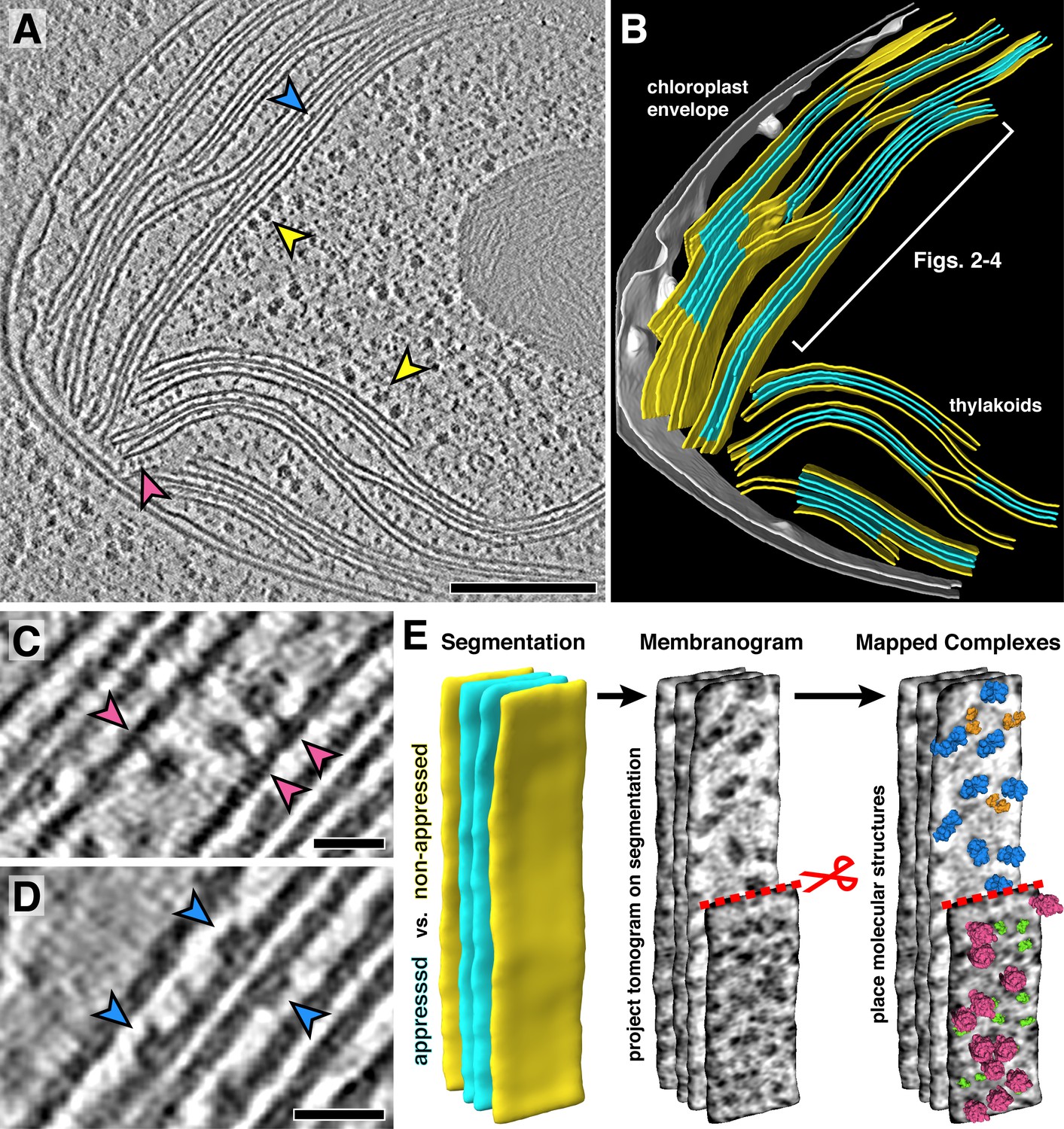
In situ cryo-electron tomography reveals the native molecular architecture of thylakoid membranes.
(A) Slice through a tomogram of the chloroplast within an intact Chlamydomonas cell. Arrowheads point to membrane-bound ribosomes (yellow), ATP synthase (magenta), and PSII (blue). (B) Corresponding 3D segmentation of the chloroplast volume, with non-appressed stroma-facing membranes in yellow, appressed stacked membranes in blue, and the chloroplast envelope in grey. The thylakoid region used in Figures 2–4 is indicated. (C-D) Close-up views showing individual ATP synthase (C) and PSII (D) complexes. (E) Mapping photosynthetic complexes into thylakoids using membranograms. Segmented membranes are extracted from the tomogram (left). Tomogram voxel values are projected onto the segmented surfaces, showing densities that protrude from the membranes. Here, densities ~2 nm above the membrane surface are shown (red scissors and dashed line: part of the non-appressed membrane has been removed to reveal luminal densities on the appressed membrane). Protein complexes are mapped onto membranograms based on the shapes of the densities and whether they protrude into the stromal or luminal space (blue: PSII, orange: cytb6f, green: PSI, magenta: ATP synthase). Scale bars: 200 nm in A, 20 nm in C and D. See Videos 1 and 2.
Figure 1—figure supplement 1
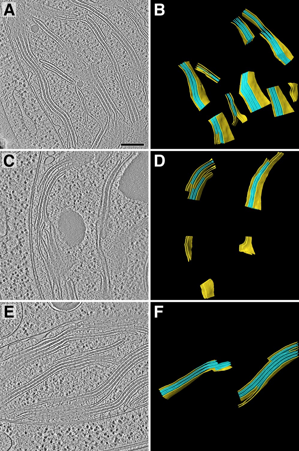
Tomogram overviews.
Overviews of the three tomograms that were analyzed in addition to the tomogram shown in Figure 1. (A, C, E) Two-dimensional slices through the tomographic volumes. (B, D, F) Three-dimensional segmented membrane regions (yellow: non-appressed, blue: appressed) where protein complexes were quantified by membranograms. Table 1 displays the total concentrations of protein complexes quantified from 84 membrane regions in the four tomograms. Scale bar: 200 nm.
Figure 1—figure supplement 2
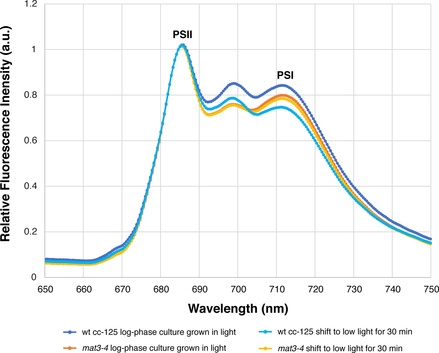
The mat3-4 strain has a similar 77K fluorescence spectrum profile to wild-type cells.
Measurements were made from log-phase cultures grown under the same conditions that were used for cryo-ET (illuminated with ~90 µmol photons m−2s−1, bubbling with normal atmosphere). 77K spectra were measured from cells taken immediately from growing cultures (dark blue: wild-type cc-125, orange: mat3-4) and from cells that were allowed to sit for 30 min in a conical tube in low light (~10 µmol photons m−2s−1), similar to the conditions that cells experienced before plunge-freezing (light blue: wild-type cc-125, yellow: mat3-4). The plot of each condition is the average of three independent biological replicates, each with five technical replicates (15 measurements total per condition). Since both strains (in both environmental conditions) have similar 77K spectra, our cryo-ET description of the arrangement of photosynthetic complexes within mat3-4 (Figures 1–4; Table 1) is likely comparable to wild-type cells. These 77K spectra are similar to previously reported spectra from Chlamydomonas cells in State I (Nawrocki et al., 2016).
Figure 2 with 4 supplements

Mapping photosynthetic complexes within appressed and non-appressed thylakoid membranes.
(A) Schematic of how each molecular complex extends from the membrane into the stroma (St) and thylakoid lumen (Lu). Into the lumen, large dimeric densities extend ~4 nm from PSII and small dimeric densities extend ~3 nm from cytb6f (b6f). Into the stroma, a small monomeric density extends ~3 nm from PSI, the F1 region of ATP synthase (ATP-S) extends ~15 nm, and thylakoid-bound ribosomes (Ribo) extend ~25 nm. (B) Three segmented thylakoids from the region indicated in Figure 1B. Membranes 1–3 (M1-M3, yellow: non-appressed, blue: appressed) are examined by membranograms. The eye symbol with arrow indicates the viewing direction for the membranograms. (C) Membranogram renderings of M1-M3. All membranograms show the densities ~2 nm above the membrane surface, except the top membranogram, which was grown to display densities ~10 nm into the stroma. Stromal surfaces are underlined with solid colors, whereas luminal surfaces are underlined with a dotted color pattern. The complexes identified in each surface are indicated on the right. (D) Model representation of M1-M3, showing the organization of all of the thylakoid complexes (colors correspond to the schematic in A). For a gallery of the different complexes visualized by membranograms, see Figure 2—figure supplement 1.
Figure 2—figure supplement 1
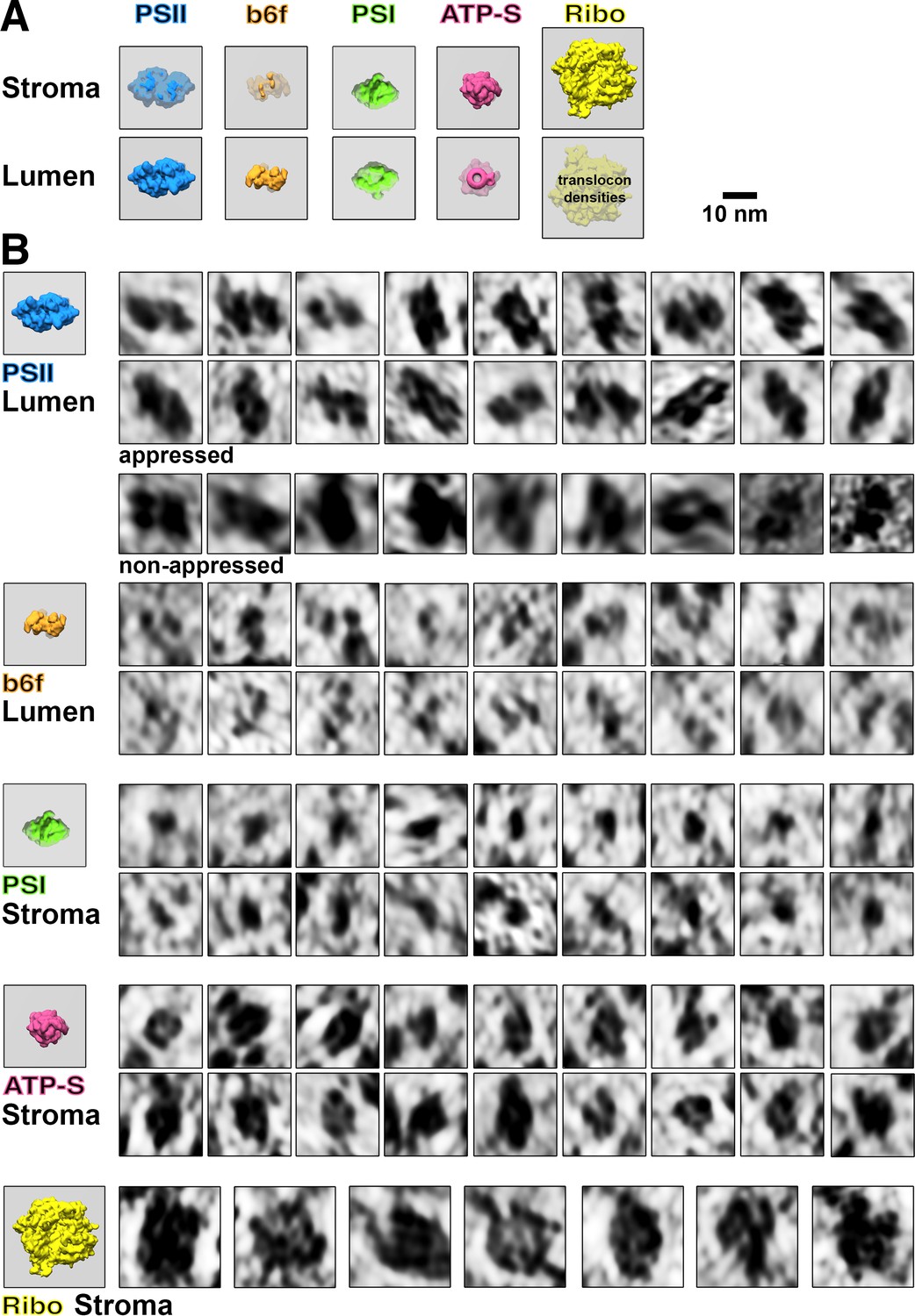
Membranogram particle gallery.
(A) Models of how each molecular complex appears when looking at the stromal and luminal surfaces of a thylakoid membrane (grey). Protruding densities are brightly colored, whereas densities located behind the membrane surface are greyer. Thylakoid-bound ribosomes would likely have small translocon densities visible on the luminal surface. Notice that outline ‘footprint’ shapes of the complexes appear mirrored when viewed through the membrane. Photosystem II = PSII, cytochrome b6f = b6f, Photosystem I = PSI, ATP synthase = ATP-S, thylakoid-bound ribosomes = Ribo. (B) Gallery of thylakoid-bound complexes as they appear in membranograms. Corresponding models of complexes protruding from the relevant membrane surface are shown on the left. Examples of PSII complexes are shown from both appressed membranes (where they are common) and non-appressed membranes (where they are very rare, see Table 1).
Figure 2—figure supplement 2
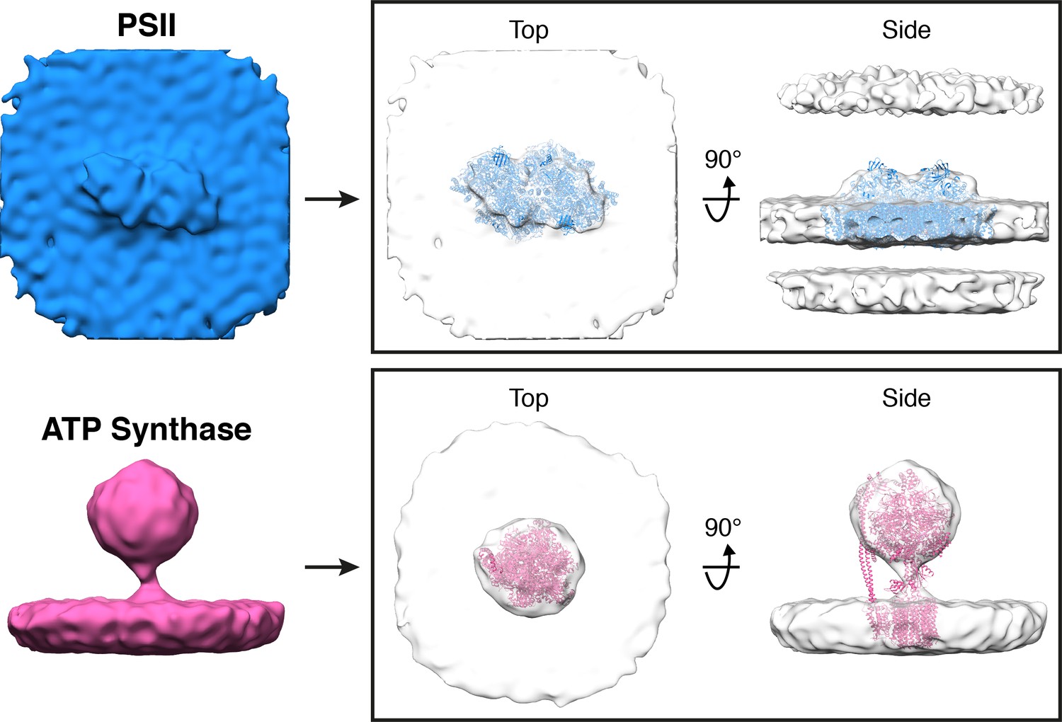
Subtomogram averages of PSII and ATP synthase generated from particle positions assigned by membranograms.
In the boxes on the right, the averages are fitted with molecular structures determined by single particle cryo-EM (PDB: 6KAD, 6FKF) (Hahn et al., 2018; Sheng et al., 2019). The subtomogram alignment did not resolve the rotationally asymmetric stator region of ATP synthase, likely because the F1 region undergoes large movements (Hahn et al., 2018) that introduce structural heterogeneity in our active, native complexes. Nevertheless, both averages closely resemble the known structures of these complexes, validating the assignment of identities by membranograms.
Figure 2—figure supplement 3
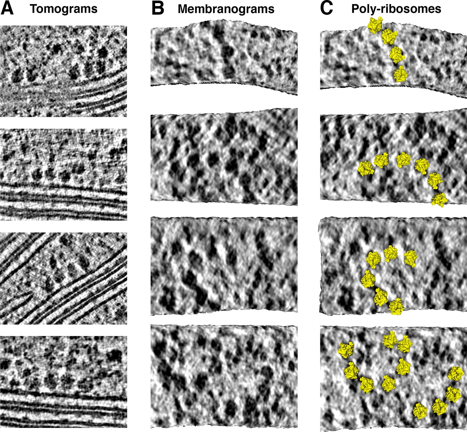
Thylakoid-bound poly-ribosome chains.
(A) Poly-ribosomes at thylakoid membranes, visualized in two-dimensional tomographic slices. (B-C) Poly-ribosome chains, ranging in length from 4 to 7 ribosomes, visualized in membranograms rendered ~10 nm from the thylakoid membrane surface. In C, chloroplast ribosome structures (PDB: 5MMM) (Bieri et al., 2017) have been mapped onto the membranograms.
Figure 2—figure supplement 4

Distributions of nearest-neighbor distances for PSII, cytb6f, ATP synthase, and membrane-associated ribosomes.
Distances were measured between the center positions of nearest-neighbor complexes within the plane of the membrane. Mean, median, and standard deviation of the mean (SD) are noted in the plots. The PSII nearest-neighbor distance is similar to a previous AFM measurement of light-adapted spinach (Wood et al., 2018), but slightly greater than AFM of dark-adapted spinach (Wood et al., 2018) and freeze-fracture of dark-adapted Arabidopsis (Goral et al., 2012). The ribosome distribution has a sharp peak at 20–25 nm. This likely corresponds to the distance between ribosomes in thylakoid-bound poly-ribosome chains (Figure 2C–D, Figure 2—figure supplement 3), as it is similar to the ~22 nm ribosome spacing in bacterial poly-ribosomes (Brandt et al., 2009).
Figure 3 with 1 supplement
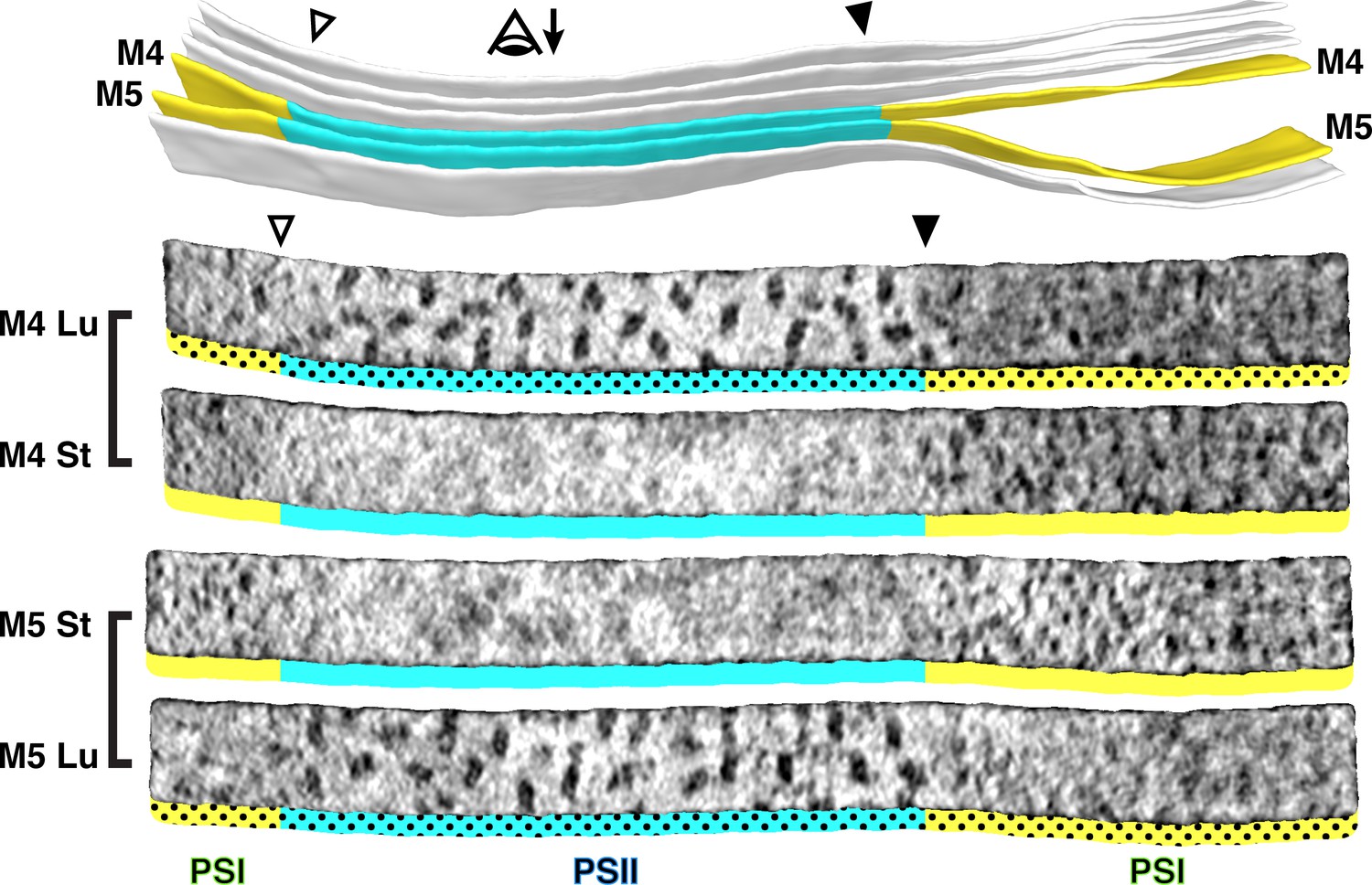
Strict segregation of PSII and PSI at transitions between appressed and non-appressed regions.
Above: Three segmented thylakoids from the region indicated in Figure 1B. Membranes 4–5 (M4 and M5, yellow: non-appressed, blue: appressed) are examined by membranograms. The eye symbol with arrow indicates the viewing direction for the membranograms. Below: Membranograms of M4 and M5. All membranograms show the densities ~2 nm above the membrane surface. Stromal surfaces are underlined with solid colors, whereas luminal surfaces are underlined with a dotted color pattern. Transitions between appressed and non-appressed regions are marked with arrowheads. PSII is exclusively found in the appressed regions, whereas PSI is exclusively found in the non-appressed regions, with sharp partitioning at the transitions between regions. For an additional example of how lateral heterogeneity of PSII and PSI is coupled to membrane architecture, see Figure 3—figure supplement 1.
Figure 3—figure supplement 1
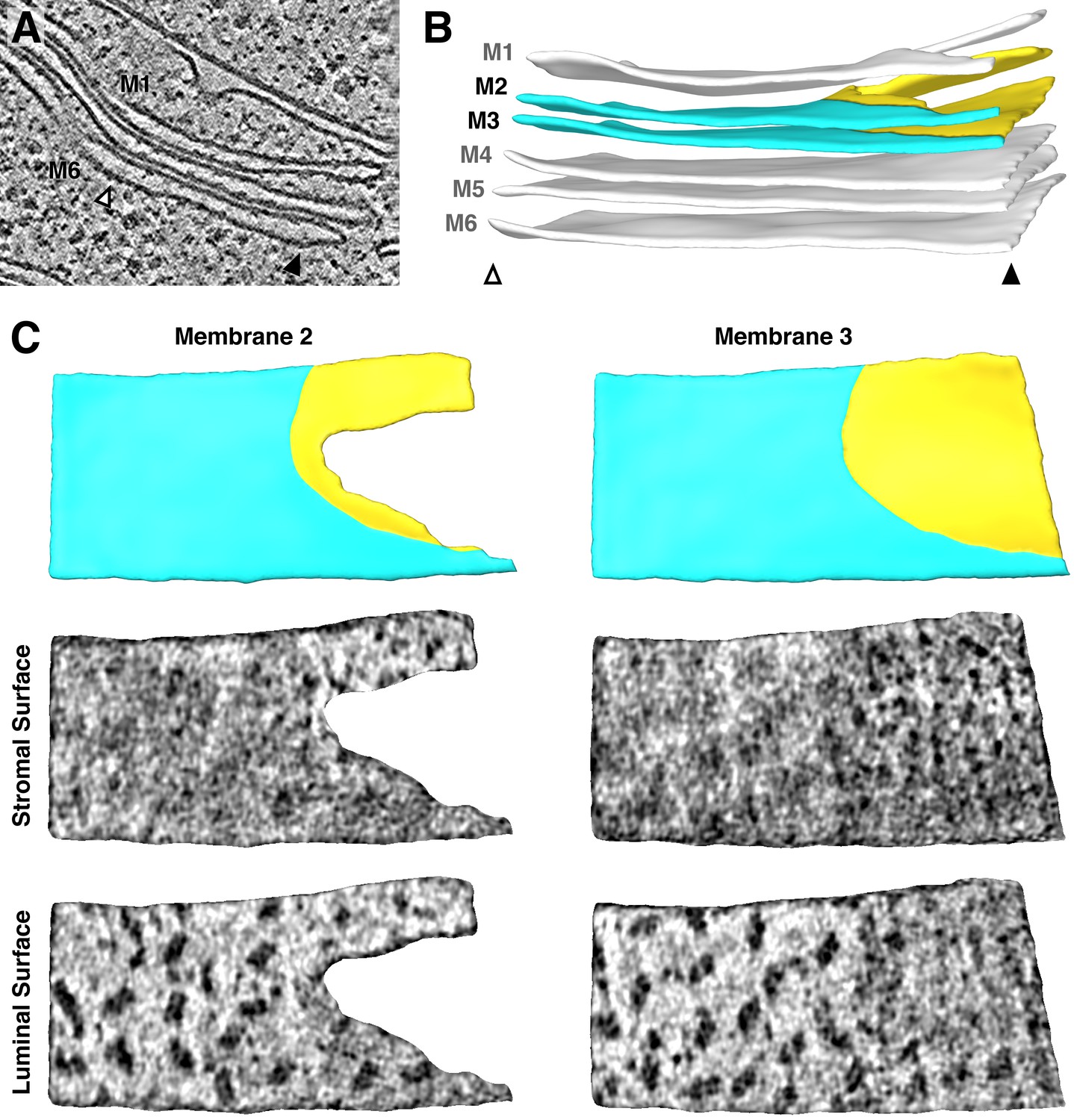
Additional example of the strict lateral heterogeneity between PSI and PSII at the transition between appressed and non-appressed membrane domains.
(A) Slice through a tomogram showing a stack of three thylakoids that splits into a stack of two thylakoids and a single thylakoid. (B) Segmentation of the thylakoid membranes in this stack. Arrowheads and membrane labels (M1-M6) correspond to the regions indicated in A. The thylakoid composed of M1 and M2 is more architecturally complex than the region shown in Figure 3. M2 and M3 (yellow: non-appressed, blue: appressed) are examined by membranograms. (C) Above: Surface views of the segmented M2 and M3, showing the appressed and non-appressed regions of these adjacent membranes. Below: Membranograms of M2 and M3, showing densities ~2 nm above the stromal and luminal surfaces. PSII is exclusively found in the appressed regions, whereas PSI is only seen in the non-appressed regions, with a sharp transition between these domains.
Figure 4 with 2 supplements
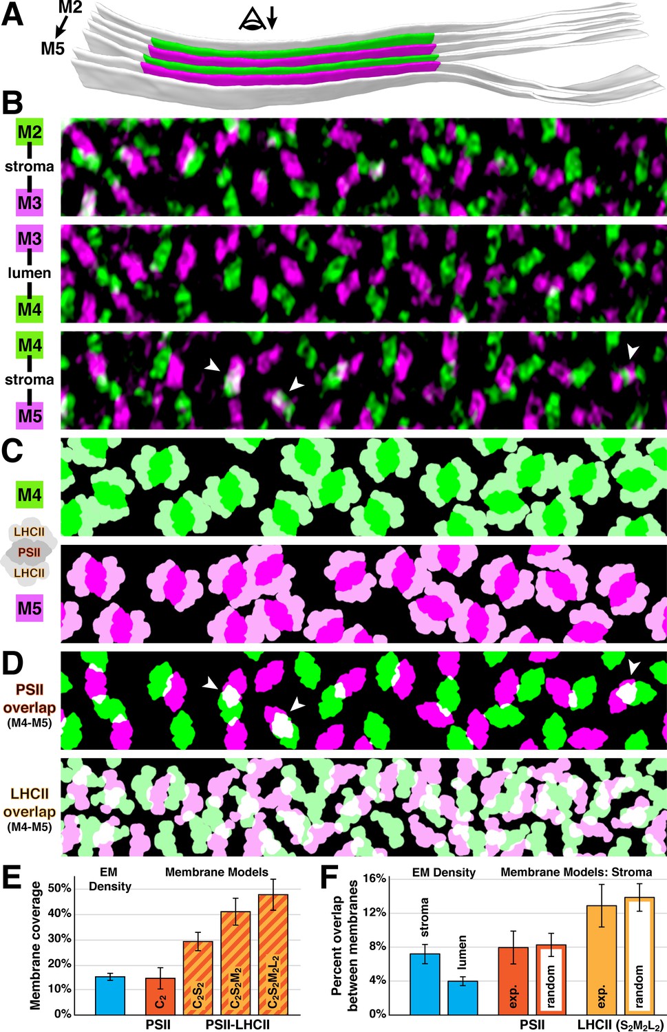
Native thylakoids can accommodate PSII-LHCII supercomplexes, which are randomly distributed across the stromal gap.
(A) Three segmented thylakoids from the region indicated in Figure 1B. Membranes 2–5 (M2 to M5, alternating green and magenta) are examined by membranograms. The eye symbol with arrow indicates the viewing direction for the membranograms. (B) Overlays of two luminal surface membranograms, superimposed across the stromal gap (M2-M3, M4-M5) and thylakoid lumen (M3-M4). Membranograms are pseudocolored corresponding to A. Overlapping PSII complexes in the M4-M5 overlay are indicated with white arrowheads. (C) Model representations of M4 and M5, with C2S2M2L2-type PSII-LHCII supercomplexes positioned according to the luminal densities observed in the membranograms. The spacing indicates that appressed thylakoids can accommodate these supercomplexes. (D) M4-M5 overlays using the membrane models from C, separately showing the PSII core complexes (top) and LHCII antennas (bottom). Overlapping regions are white. White arrowheads correspond to the overlapping complexes in B. (E) Blue bar: the percentage of membrane surface area occupied by luminal EM density (15.0 ± 1.2%, N = 19 membranes) in membranograms (e.g., panel B). Red and red/yellow striped bars: the percentage of surface area in membrane models (e.g., panel C) occupied by C2-type PSII core complexes (14.6 ± 4.1%) and C2S2-type (29.1 ± 3.7%), C2S2M2-type (40.7 ± 5.2%), and C2S2M2L2-type (47.3 ± 6.0%) PSII-LHCII supercomplexes (N = 9 membranes). (F) Blue bars: the percentage of luminal EM density in membranograms that overlaps between adjacent appressed membranes spanning the stromal gap (7.2 ± 1.1%, N = 11 overlays) and thylakoid lumen (4.0 ± 0.5%, N = 6 overlays). See Figure 4—figure supplement 1 for how the EM density was thresholded to calculate surface area and overlap. Red and yellow bars: using membrane models with C2S2M2L2-type PSII-LHCII supercomplexes, the percentage of PSII and LHCII surface area that overlaps between adjacent appressed membranes spanning the stromal gap (N = 4 overlays). The experimental measurements (exp.; PSII: 8.0 ± 1.9%, LHCII: 12.9 ± 2.5%) and simulations of complexes randomly positioned within the membrane (random; PSII: 8.3 ± 1.4%, LHCII: 13.8 ± 1.6%, N = 100 simulations per overlay) were not significantly different (p>0.05 from t-tests with Welch’s correction for unequal variances: p=0.512 for PSII, p=0.762 for LHCII). See Figure 4—figure supplement 2 and Materials and methods for how the random simulations were performed. Error bars denote standard deviation.
Figure 4—figure supplement 1
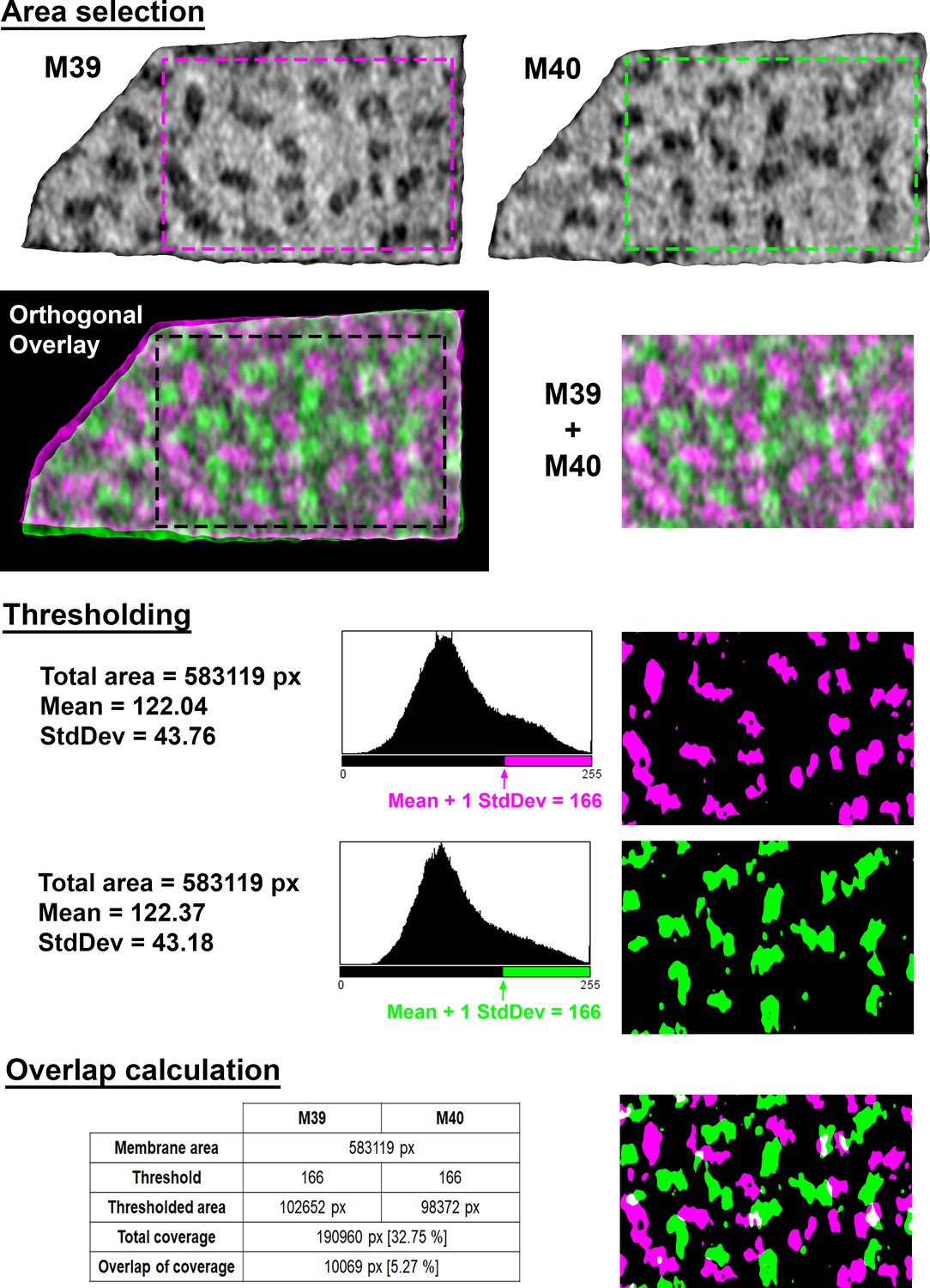
Calculations of membrane coverage and intermembrane overlap from EM density.
Area selection: To select overlapping areas of two adjacent membranes (M39 and M40 in this example; magenta and green, respectively), the two membranograms are overlaid along a vector orthogonal to both membrane surfaces. The overlay is then cropped to prevent edge effects (M39 + M40). Thresholding: Each cropped membranogram is binarized, with the threshold defined by the mean pixel value plus one standard deviation (StdDev), rounded to the nearest integer value. Overlap calculation: The percentage of each membrane occupied by EM densities was calculated as the number of thresholded pixels (green or magenta) divided by total pixels in the membrane (black + green or magenta). The percentage of overlapping EM density was calculated as the overlapping thresholded pixels (white) divided by the sum of the thresholded pixels in both membranes (white + green + magenta). Overlapping pixels were only counted once in this summation of all thresholded pixels.
Figure 4—figure supplement 2
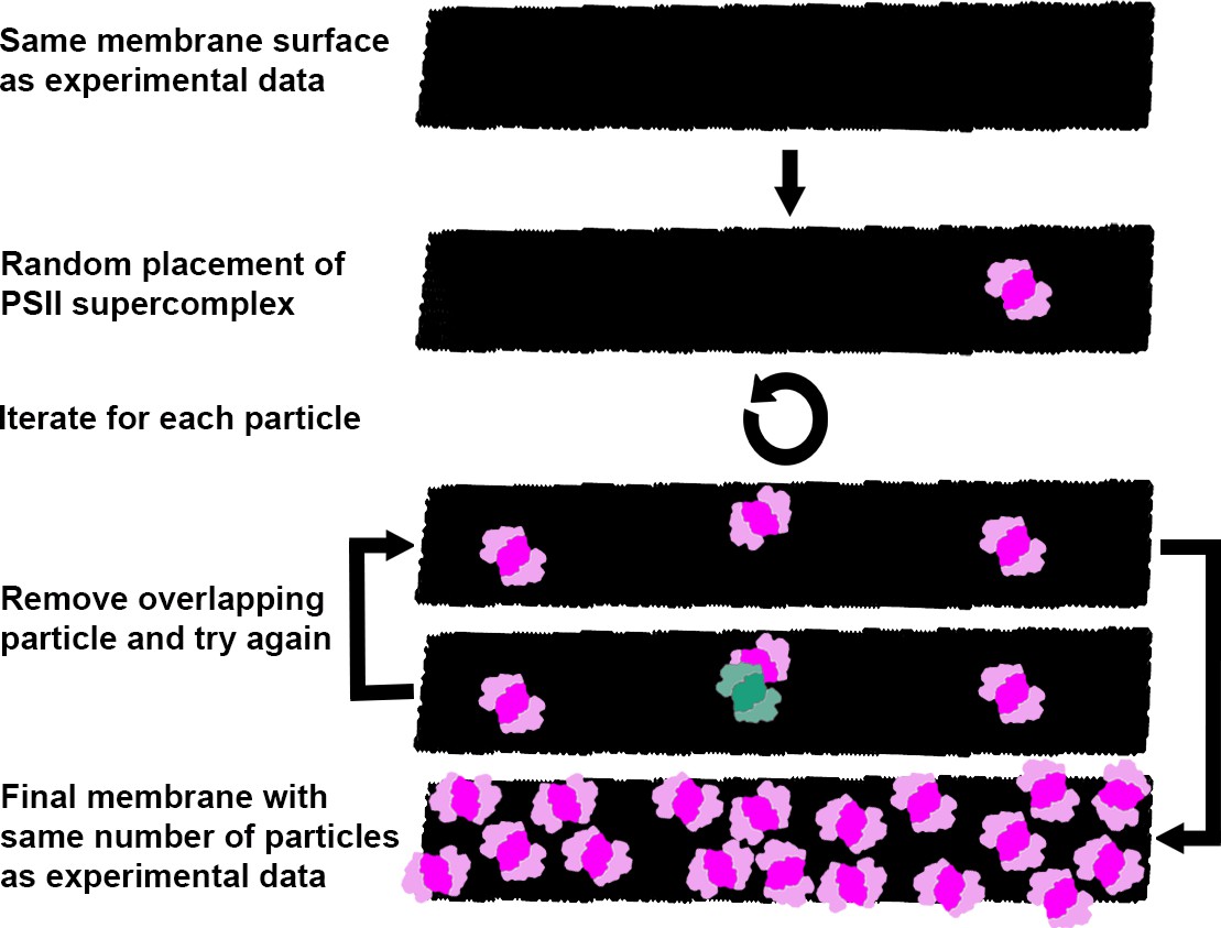
Generation of random membrane models.
Schematic representation of the workflow for generating membranes with randomly distributed C2S2M2L2-type PSII-LHCII supercomplexes, used for the analysis of intermembrane PSII and LHCII overlap (Figure 4F). The same number of supercomplexes (pink) as measured experimentally were placed one-by-one with random positions and orientations into the same membrane surface (black). If a new particle overlapped with a particle that had already been placed (event in blue/green), it was removed and placed again until it fit without overlap. The random distributions were simulated 100 times for each membrane. While diagrammed in 2D here for visual simplicity, the process was actually performed on 3D membranes (see Materials and methods).
Videos
Video 1
In situ cryo-electron tomography reveals native thylakoid architecture with molecular clarity.
Sequential slices back and forth in Z through the tomographic volume shown in Figure 1A. The yellow boxed region, focusing on the thylakoids shown in Figures 2–4, is then enlarged and displayed in the lower right corner of the video. Ribosomes and ATP synthase complexes can be seen bound to the stromal non-appressed thylakoid surfaces, while densities from PSII and cytb6f extend from the appressed surfaces into the thylakoid lumen.
Video 2
Mapping molecular complexes into thylakoid architecture with membranograms.
Tomographic densities are projected onto the surface of a 3D membrane segmentation to produce a membranogram. The segmentation can be interactively grown and shrunk to visualize densities at different distances from the membrane. The bottom part of the video shows a membranogram of the luminal surface of an appressed thylakoid membrane. In the top part of the video, a moving red arrow indicates the position of the membranogram surface relative to the thylakoid architecture (shown both as real data and corresponding illustration). The video begins by growing and shrinking the segmentation, showing densities that begin within the appressed membrane and extend into the thylakoid lumen. Growing and shrinking the segmentation immediately adjacent to the membrane surface allows careful inspection of the thylakoid-bound densities. First, the positions and orientations (boxes with vector lines) of the PSII and cytb6f (b6f) complexes are assigned. To-scale 3D structures of both complexes are then mapped onto the membranogram, showing good overlap with the tomographic densities.
Tables
Table 1
Average concentrations of macromolecular complexes in native Chlamydomonas thylakoid membranes.
| Concentration of complexes [average number of complexes per square micrometer] | |||||||
|---|---|---|---|---|---|---|---|
| PSII | Cytb6f | PSI | ATP-S | Ribo | Unknown | Total | |
| Non-appressed | 24 | 501* | 1049* | 1652 | 113 | 1568 | 4907 |
| Appressed | 1122 | 631 | 2 | 0 | 0 | 170 | 1925 |
-
N = 84 membrane regions (51 non-appressed and 33 appressed) from four tomograms. ‘Unknown’ densities are particles that could not be assigned an identity, including particles found near the edges of the segmented membrane regions. Asterisks show classes of complexes that were identified with lower confidence. PSII densities are dimers, and thus the monomeric stoichiometry of PSII/PSI is 2.14. Densities that could correspond to free PSII monomers were seldom observed in membranograms and thus were not assigned.
Additional files
Download links
A two-part list of links to download the article, or parts of the article, in various formats.
Downloads (link to download the article as PDF)
Open citations (links to open the citations from this article in various online reference manager services)
Cite this article (links to download the citations from this article in formats compatible with various reference manager tools)
Charting the native architecture of Chlamydomonas thylakoid membranes with single-molecule precision
eLife 9:e53740.
https://doi.org/10.7554/eLife.53740


