Impact of community piped water coverage on re-infection with urogenital schistosomiasis in rural South Africa
- Africa Health Research Institute, South Africa
- School of Nursing and Public Health, University of KwaZulu-Natal, South Africa
- KwaZulu-Natal Innovation and Sequencing Platform (KRISP), University of KwaZulu-Natal, South Africa
- Heidelberg Institute of Global Health, Faculty of Medicine, University of Heidelberg, Germany
- Department of Geography and Geographic Information Science, University of Cincinnati, United States
- Health Geography and Disease Modeling Laboratory, University of Cincinnati, United States
- School of Life Sciences, University of KwaZulu-Natal, South Africa
- Lincoln International Institute for Rural Health, University of Lincoln, United Kingdom
Figures
Figure 1
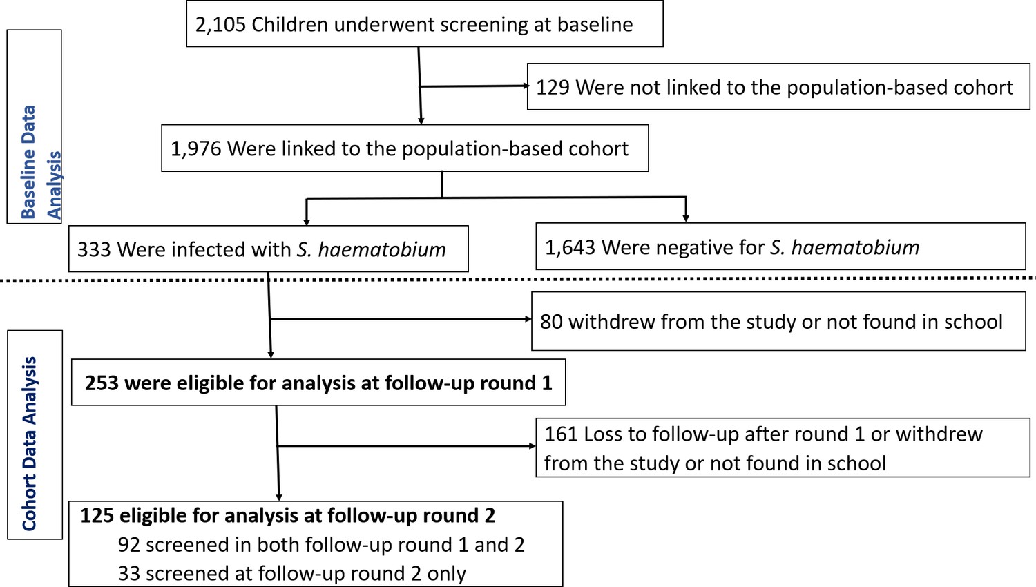
Baseline screening for Schistosoma haematobium infection and re-infection follow-up rounds of the study participants.
Participants who were not linked to the population-based cohort study were excluded from the baseline analysis presented in our previous analyses (Tanser et al., 2018) and those not treated for infection at baseline were excluded from the re-infection analysis. Participants who were treated at baseline but not screened at round 1 were eligible for screening at round 2 if they provided informed consent.
Figure 2
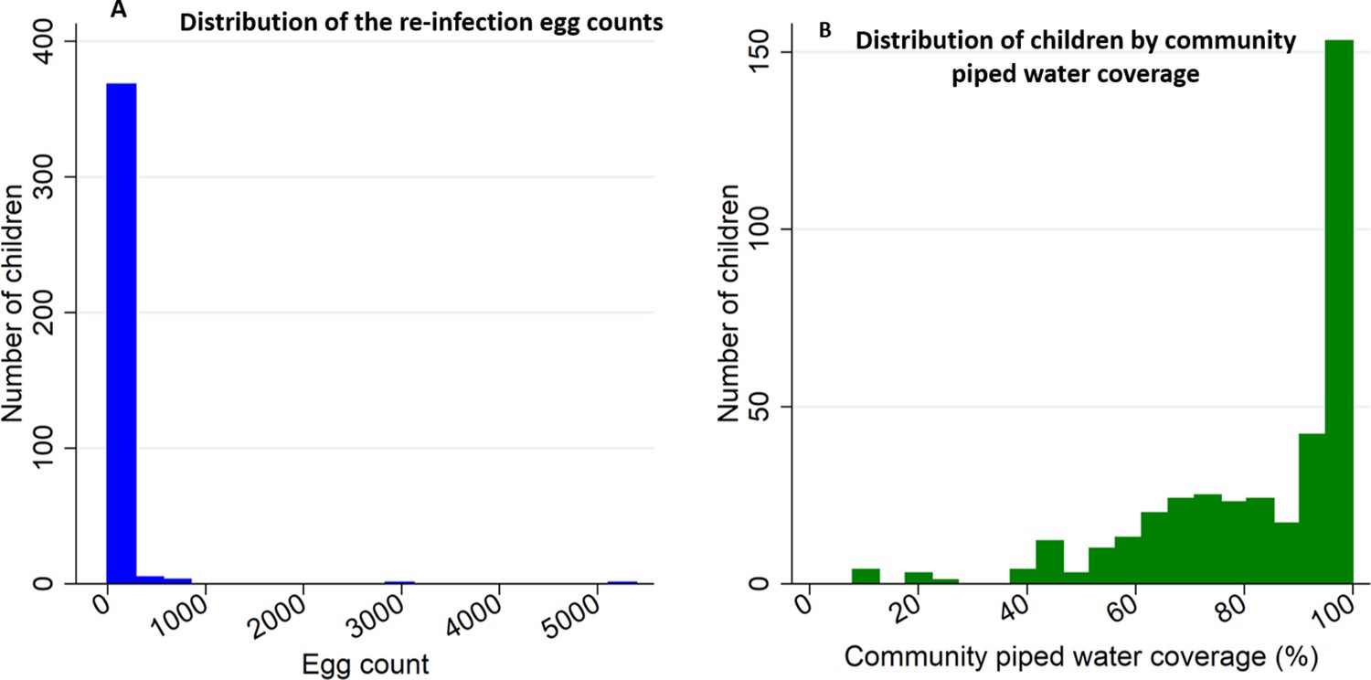
Histograms of Schistosoma haematobium egg counts and community piped water coverage for the re-infection cohort participants (n = 378).
Panel (A) shows the distribution of egg counts/10 mL among children observed at follow-up round 1 and 2, and panel (B) shows the distribution of community piped water coverage among all study participants. Community piped water coverage in the community surrounding each child was derived from the population-based 2007 piped water use survey conducted in all households in the study area.
Figure 3
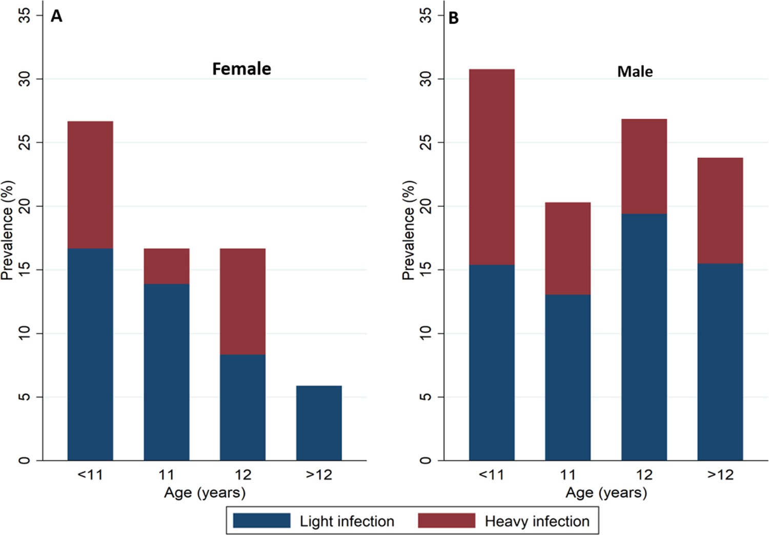
Prevalence of Schistosoma haematobium re-infection and intensity of re-infection by age and sex among children taking part in the re-infection cohort (n = 378).
Blue represents light re-infections (<50 eggs per 10 ml urine) and Red represents heavy re-infections (≥50 eggs per 10 ml urine). Panels A and B show the prevalence of Schistosoma haematobium for female and male children respectively.
Figure 4
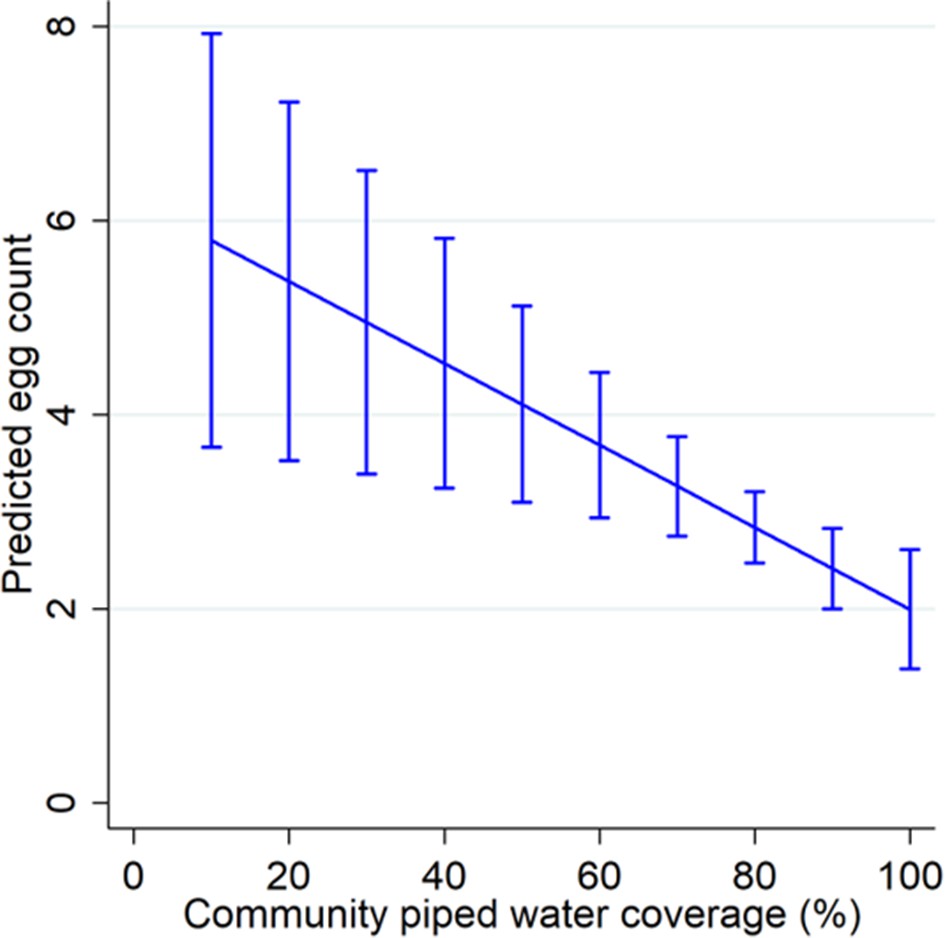
Margin plot of piped water coverage and re-infection intensity.
The margin plot was constructed from the final parsimonious multivariable negative binomial regression model for the pooled dataset (n = 378, incidence rate ratio = 0.96, p=0.004). Piped water coverage was estimated using the Gaussian kernel density methodology.
Figure 5
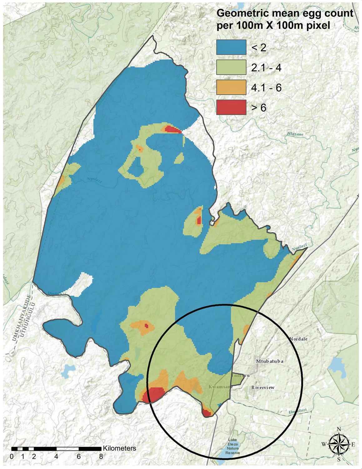
Geospatial heterogeneity in Schistosoma haematobium geometric mean egg counts (intensity of re-infection) across the study area.
The map shows the geographical distribution of mean egg counts/10 mL estimated using the Gaussian kernel of 3 km radius for the pooled re-infection cohort datasets (n = 378). Superimposed on the map is the local cluster (radius = 6.93 km, geometric mean egg count = 54.95, p=0.006) detected using Kulldorff’s spatial scan statistic.
Figure 6
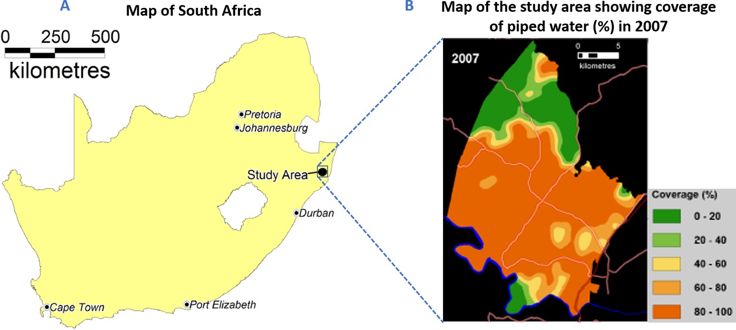
Location of the study area in South Africa.
Panel A displays the map of South Africa highlighting the major towns and the location of the study area. Panel B displays the map of the study area showing the major roads and the coverage of piped water (%) in 2007. Community piped water coverage was estimated using the Gaussian kernel methodology (Tanser et al., 2018).
Tables
Table 1
Characteristics of children enrolled in the re-infection cohort.
| Follow-up round 1 (N = 253) | Follow-up round 2 (N = 125) | |||||
|---|---|---|---|---|---|---|
| Total | Infected n(%) | (95% CI) | Total | Infected n(%) | (95% CI) | |
| Overall | 253 | 61 (24.1) | (19.0–29.9) | 125 | 24 (19.2) | (12.7–27.2) |
| Gender | ||||||
| Female | 86 | 16 (18.6) | (11.0–28.4) | 33 | 5 (15.2) | (5.1–31.9) |
| Male | 167 | 45 (27.0) | (20.4–34.3) | 92 | 19 (20.7 | (12.9–30.4) |
| Age group | ||||||
| ≤10 | 41 | 13 (31.7) | (18.1–48.1) | 28 | 7 (25.0) | (10.7–44.9) |
| 11 | 71 | 15 (21.1) | (12.3–32.4) | 34 | 5 (14.7) | (5.0–31.1) |
| 12 | 74 | 18 (24.3) | (15.1–35.7) | 29 | 6 (20.7) | (8.0–39.7) |
| ≥13 | 67 | 15 (22.4) | (13.1–34.2) | 34 | 6 (17.6) | (6.8–34.5) |
| Community piped water coverage (%) | ||||||
| <70 | 58 | 17 (29.3) | (18.1–42.7) | 31 | 5 (16.1) | (5.5–33.7) |
| 70 - < 90 | 66 | 13 (19.7) | (10.9–31.3) | 28 | 8 (28.6) | (13.2–48.7) |
| ≥90 | 129 | 31 (24.0) | (16.9–32.3) | 66 | 11 (16.6) | (8.6–27.9) |
| Altitude class (meters) | ||||||
| <50 | 17 | 5 (29.4) | (10.3–56.0) | 14 | 6 (42.9) | (17.7–71.1) |
| 50–100 | 140 | 31 (22.1) | (15.6–29.9) | 62 | 11 (17.7) | (9.2–29.5) |
| 100–150 | 84 | 21 (25.0) | (16.2–35.6) | 42 | 5 (11.9) | (4.0–25.6) |
| 150–200 | 7 | 2 (28.6) | (3.7–71.0) | 3 | 0 (0) | (0–70.8) |
| ≥200 | 5 | 2 (40.0) | (5.3–85.3) | 4 | 2 (50.0) | (6.8–93.2) |
| Distance water body class | ||||||
| <1 km | 92 | 20 (21.7) | (13.8–31.6) | 46 | 11 (23.9) | (12.6–38.8) |
| 1–2 km | 98 | 25 (25.5) | (17.2–35.3) | 42 | 8 (19.1) | (8.6–34.1) |
| 2–3 km | 46 | 13 (28.3) | (16.0–43.5) | 26 | 5 (19.2) | (6.6–39.4) |
| >3 km | 17 | 3 (17.7) | (3.8–43.4) | 11 | 0 (0) | (0–28.5) |
| School grade | ||||||
| Grade 5 | 144 | 37 (25.7) | (18.8–33.6) | 74 | 13 (17.6) | (9.7–28.2) |
| Grade 6 | 109 | 24 (22.0) | (14.6–31.0) | 51 | 11 (21.6) | (11.3–35.3) |
| Toilet | ||||||
| No Toilet | 47 | 13 (27.7) | (15.6–42.6) | 23 | 1 (4.3) | (0.1–21.9) |
| Toilet | 206 | 48 (23.3) | (17.7–29.7) | 102 | 23 (22.6) | (14.9–31.9) |
| Land cover classification | ||||||
| Closed shrubland | 145 | 35 (24.1) | (17.4–31.9) | 65 | 12 (18.5) | (9.9–30.0) |
| Open shrubland | 59 | 14 (23.7) | (13.6–36.6) | 34 | 6 (17.7) | (6.8–34.5) |
| Sparse shrubland | 41 | 11 (26.8) | (14.2–42.9) | 19 | 6 (31.6) | (12.6–56.6) |
| Thickett | 8 | 1 (12.50) | (0.3–52.7) | 7 | 0 (0) | (0–41.0) |
| Baseline intensity of infection | ||||||
| Light infection | 105 | 35 (33.3) | (24.4–43.2) | 50 | 12 (24.0) | (13.1–38.2) |
| Heavy infection | 148 | 26 (17.6) | (11.8–24.7) | 75 | 12 (16.0) | (8.6–26.3) |
| Sample size (N) | 253 | 125 | ||||
Table 2
Predictors of intensity of re-infection with Schistosoma haematobium (pooled analysis, n = 378).
Model 1 presents results from the univariable negative binomial model and Model 2 presents results from the final parsimonious multivariable negative binomial model. Homestead level piped water coverage was derived from a Gaussian kernel density estimation using data from a survey conducted in 2007.
| Model 1: univariable (n = 378) | Model 2: multivariable (n = 378) | |||||
|---|---|---|---|---|---|---|
| Covariates | IRR | 95% | P-value | IRR | 95% | P-value |
| Female | 0.17 | 0.06–0.54 | 0.003 | 0.14 | 0.06–0.32 | <0.001 |
| Community piped water coverage (continuous effect) | 0.96 | 0.93–0.98 | 0.002 | 0.96 | 0.93–0.98 | 0.004 |
| Age at baseline (years) | 0.68 | 0.50–0.93 | 0.017 | 0.78 | 0.59–1.04 | 0.094 |
| Altitude class (ref < 50) | ||||||
| 50–100 | 3.65 | 0.91–14.5 | 0.067 | 1.20 | 0.31–4.56 | 0.793 |
| 100–150 | 0.72 | 0.21–2.54 | 0.612 | 0.41 | 0.1–1.74 | 0.226 |
| ≥150 | 0.11 | 0.02–0.62 | 0.012 | 0.05 | 0.01–0.32 | 0.001 |
| Land cover class (ref. Sparse shrubland) | ||||||
| Closed shrubland | 1.96 | 0.51–7.57 | 0.327 | 0.86 | 0.34–2.21 | 0.754 |
| Open shrubland/grassland | 1.77 | 0.33–9.49 | 0.508 | 1.41 | 0.48–4.16 | 0.533 |
| Thickett | 0.01 | 0.00–0.06 | <0.001 | 0.02 | 0.00–0.20 | 0.001 |
| Toilet in household (ref. no toilet) | 2.71 | 0.70–10.4 | 0.148 | 0.77 | 0.24–2.46 | 0.662 |
| Grade (ref. Grade 5) | 0.24 | 0.08–0.75 | 0.014 | 1.35 | 0.52–3.48 | 0.540 |
| Visit (ref. Follow up 1) | 1.01 | 0.21–4.92 | 0.989 | 0.74 | 0.31–1.76 | 0.494 |
| Distance to water body class (ref. < 1 km) | ||||||
| 1–2 km | 0.11 | 0.03–0.34 | <0.001 | |||
| 2–3 km | 0.18 | 0.04–0.85 | 0.031 | |||
| >3 km | 0.08 | 0.01–0.54 | 0.010 | |||
| Household wealth index (ref. 1st quintile) | ||||||
| 2 | 3.75 | 0.49–28.7 | 0.203 | |||
| 3 | 0.38 | 0.08–1.83 | 0.233 | |||
| 4 | 3.22 | 0.63–16.3 | 0.159 | |||
| 5 | 1.71 | 0.03–1.70 | 0.432 | |||
| Square root of slope | 0.77 | 0.45–1.32 | 0.340 | |||
| Baseline intensity of infection (ref. Light infection) | 2.59 | 0.81–8.30 | 0.110 | |||
| Alpha (overdispersion parameter) | 22.6 | 17.9–28.3 | <0.001 | |||
Additional files
-
Source data 1
Prevalence of re-infection, intensity of re-infection and re-infection rate (per 100-person year of follow-up) among individuals treated at baseline for S. haematobium infection.
- https://cdn.elifesciences.org/articles/54012/elife-54012-data1-v2.docx
-
Supplementary file 1
Predictors of Schistosoma haematobium re-infection using data from follow up round 1 only.
Model 1 presents results from a univariable negative binomial model and Model 2 presents results from a multivariable negative binomial model (N = 253).
- https://cdn.elifesciences.org/articles/54012/elife-54012-supp1-v2.docx
-
Supplementary file 2
Predictors of Schistosoma haematobium re-infection using data from follow up round 2 only.
Model 1 presents results from a univariable negative binomial and Model 2 presents results from a multivariable negative binomial model (N = 125).
- https://cdn.elifesciences.org/articles/54012/elife-54012-supp2-v2.docx
-
Supplementary file 3
Characteristics of participants who dropped out of the study at follow-up round 1.
Piped water coverage (exposure variable) was similar between participants who dropped out of the study and those that were enrolled and examined. Significantly higher dropouts were only observed among participants residing further from water bodies. Piped water coverage was derived from the Gaussian kernel density estimation of radius three kilometers.
- https://cdn.elifesciences.org/articles/54012/elife-54012-supp3-v2.docx
-
Supplementary file 4
Characteristics of participants who dropped out of the study at follow-up round 2.
Piped water coverage (exposure variable) was similar between participants who dropped out of the study and those that were enrolled and examined. Significantly higher dropouts were only observed among girls. Piped water coverage was derived from the Gaussian kernel density estimation of radius three kilometers.
- https://cdn.elifesciences.org/articles/54012/elife-54012-supp4-v2.docx
-
Transparent reporting form
- https://cdn.elifesciences.org/articles/54012/elife-54012-transrepform-v2.docx
Download links
A two-part list of links to download the article, or parts of the article, in various formats.
Downloads (link to download the article as PDF)
Open citations (links to open the citations from this article in various online reference manager services)
Cite this article (links to download the citations from this article in formats compatible with various reference manager tools)
Impact of community piped water coverage on re-infection with urogenital schistosomiasis in rural South Africa
eLife 9:e54012.
https://doi.org/10.7554/eLife.54012


