Figures and data in Efficient coding of natural scene statistics predicts discrimination thresholds for grayscale textures

Figures
Tables
Additional files

12 figures, 2 tables and 1 additional file

Figures

Figure 1

Download asset Open asset

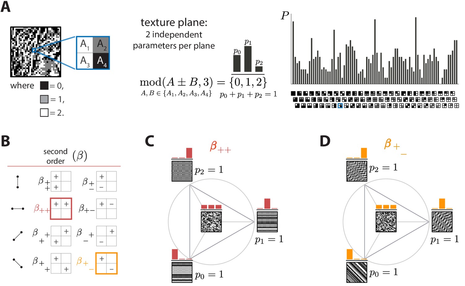
Ternary texture analysis.

(A) With three luminance levels there are $3^{4} = 81$ possible check configurations for a $2 \times 2$ block (histogram on the right). We parametrize the pairwise correlations within these blocks using modular sums or differences of luminance values at nearby locations, $m o d (A \pm B, 3)$ (see Materials and methods and Appendix 1 for details). This notation denotes the remainder after division by 3, so that for example $m o d (4, 3) = 1$ and $m o d (- 1, 3) = 2$ . The texture coordinates are defined by the probabilities $p_{0}$ , $p_{1}$ , $p_{2}$ with which $m o d (A \pm B, 3)$ equals its three possible values, 0, 1, or 2. These three probabilities must sum to 1, so there are only two independent coordinates for each triplet of probabilities. (B) The eight second-order groups (planes) of texture coordinates in the ternary case. A texture group is identified by the choice of orientation of the pair of checks for which the correlation is calculated, and by whether a sum or a difference of luminance values is used. The greek letter notation ( $β$ for the second-order planes) mirrors the notation used in Hermundstad et al., 2014. (C and D) Example texture groups (‘simple’ planes). The origin is the point $p_{0} = p_{1} = p_{2} = 1 / 3$ , representing an unbiased random texture. The interior of the triangle shows the allowed range in the plane where all the probability values are non-negative. The vertices are the points where only one of the probabilities is nonzero. An example texture patch is shown for the origin, as well as for each of the vertices of the probability space.

Figure 2

Download asset Open asset

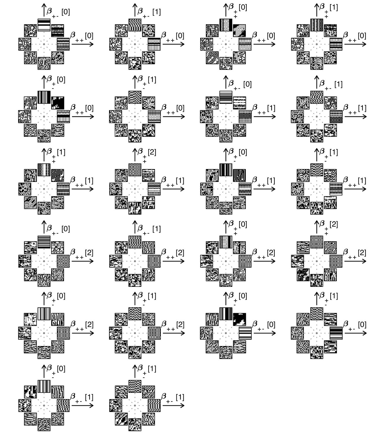
Examples of textures from all the mixed planes for which psychophysics data are available.

Each patch is obtained by choosing coordinates in two different texture groups: for instance, a point in the $(β_{+ +} [0], β_{+ -} [1])$ plane (row 1, column 2) corresponds to choosing the probabilities that $m o d (A + B, 3) = 0$ and $m o d (A - B, 3) = 1$ . Apart from these constraints, the texture is generated to maximize entropy (see Materials and methods and Appendix 2). The center of the coordinate system in all planes corresponds to an unbiased texture (i.e., the probability for each direction is 1/3), while a mixed-plane coordinate equal to one corresponds to full saturation (i.e., the probability for that direction is 1). The dashed lines indicate the directions in texture space along which the illustrated patches were generated. The patches within a given plane are drawn at a constant distance from the center, but the precise amount of texture saturation varies, according to the largest saturation that could be generated in each direction. Note that along some directions, the maximum saturation is limited by the way in which the texture coordinates are defined, or by the texture synthesis procedure (see Appendix 2).

Figure 3

Download asset Open asset

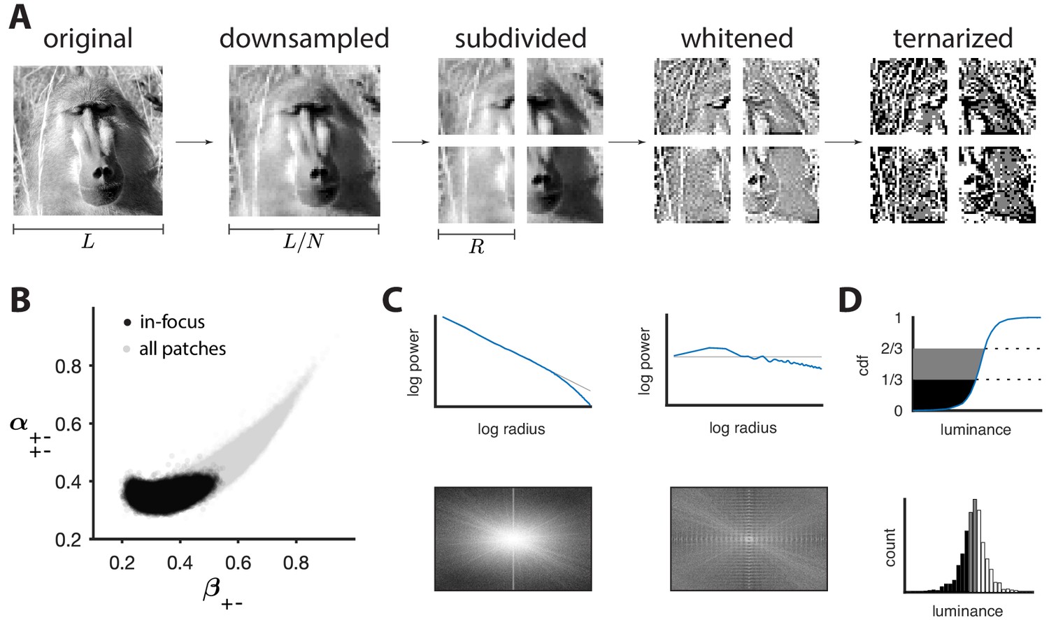
Preprocessing of natural images.

(A) Images (which use a logarithmic encoding for luminance) are first downsampled by a factor $N$ and split into square patches of size $R$ . The ensemble of patches is whitened by applying a filter that removes the average pairwise correlations (see panel C), and finally ternarized after histogram equalization (see panel D). (B) Blurry images are identified by fitting a two-component Gaussian mixture to the full distribution of image textures (shown in light gray). This is shown here in a particular projection involving a second-order direction ( $β_{+ -}$ ) and a fourth-order one $(α_{\binom{+ -}{+ -}})$ . The texture analysis is restricted to the component with higher contrast, which is shown in black on the plot. Note that a value of 1/3 on each axis corresponds to the origin of the texture space. (C) Power spectrum before and after filtering an image from the dataset. (D) Images are ternarized such that within each patch a third of the checks are converted to black, a third to gray, and a third to white. The processing pipeline illustrated here extends the analysis of Hermundstad et al., 2014 to multiple gray levels.

Figure 4

Download asset Open asset

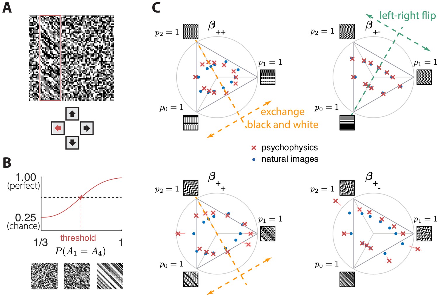
Experimental setup and results in second-order simple planes.

(A) Psychophysical trials used a four-alternative forced-choice task in which the subjects identified the location of a strip sampled from a different texture on top of a background texture. (B) The subject’s performance in terms of fraction of correct answers was fit with a Weibull function and the threshold was identified at the mid-point between chance and perfect performance. Note that if the subject’s performance never reaches the mid-point on any of the trials, this procedure may extrapolate a threshold that falls outside the valid range for the coordinate system (see, e.g., the points outside the triangles in panel C). This signifies a low-sensitivity direction of texture space. (C) Measured thresholds (red crosses with pink error bars; the error bars are in most cases smaller than the symbol sizes) and predicted thresholds (blue dots) in second-order simple planes. Thresholds were predicted to be inversely proportional to the standard deviation observed in each texture direction in natural images. The plotted results used downsampling factor $N = 2$ and patch size $R = 32$ . A single scaling factor for all planes was used to match to the psychophysics. The orange and green dashed lines show the effect of two symmetry transformations on the texture statistics (see text).

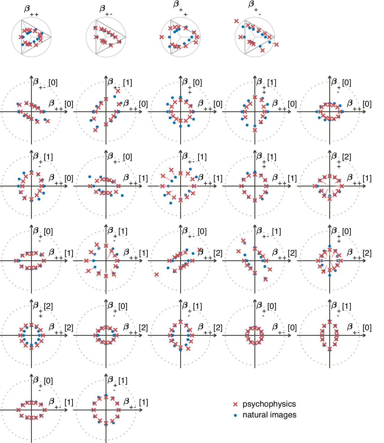
Figure 5

Download asset Open asset

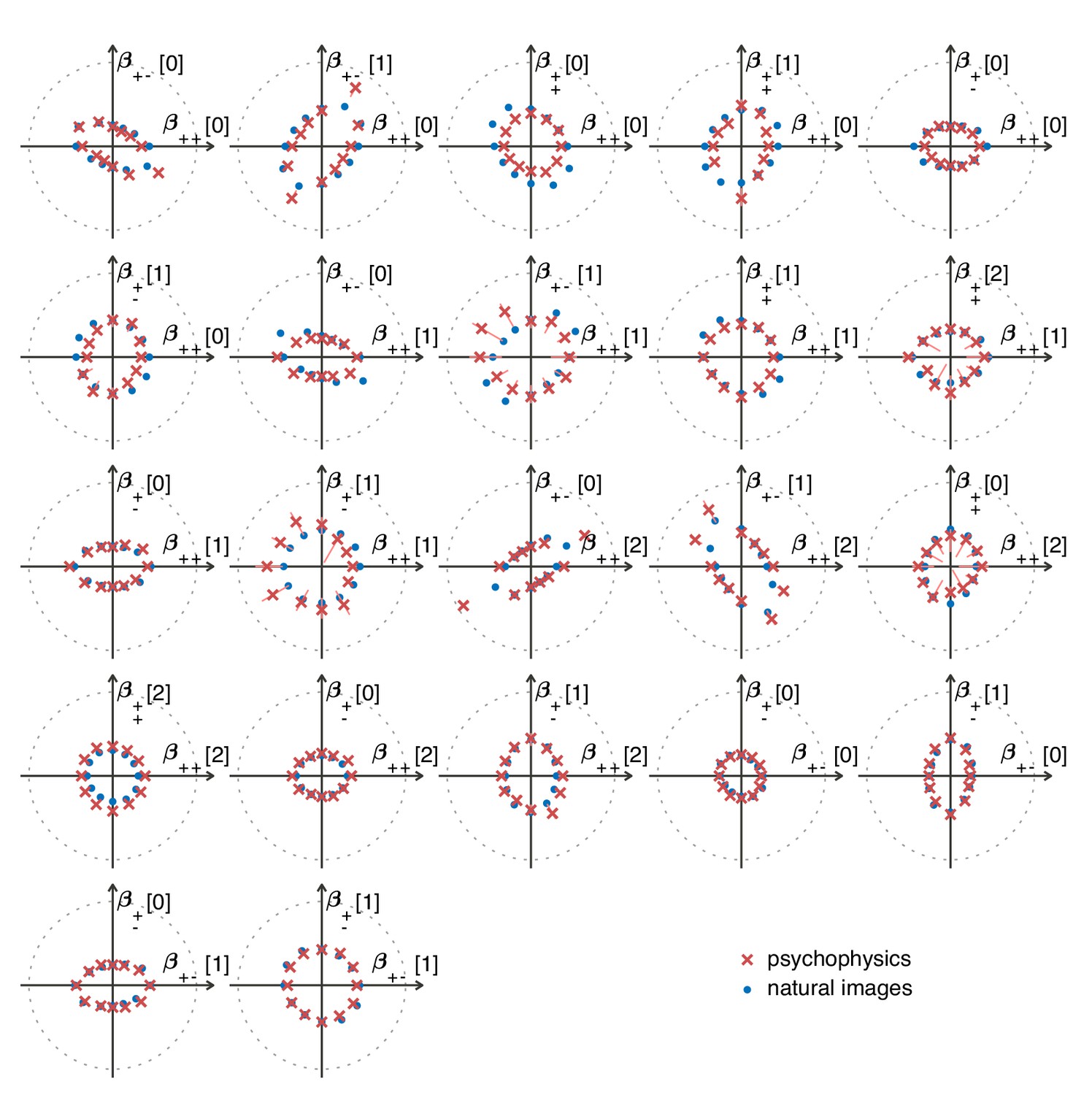
The match between measured (red crosses and error bars) and predicted (blue dots) thresholds in 22 mixed planes.

Each plot corresponds to conditions in which the coordinates in two different texture groups are specified, according to the axis labels. For instance, column two in row one is the $(β_{+ +} [0], β_{+ -} [1])$ plane; the two coordinates correspond to choosing the probabilities that $m o d (A + B, 3) = 0$ and $m o d (A - B, 3) = 1$ . As in Figure 2, the center of the coordinate system in these planes corresponds to an unbiased texture (i.e., the probability for each direction is 1/3), while a coordinate equal to 1—indicated by the gray dotted circle—corresponds to full saturation (i.e., the probability for that direction is 1).

Figure 6

Download asset Open asset

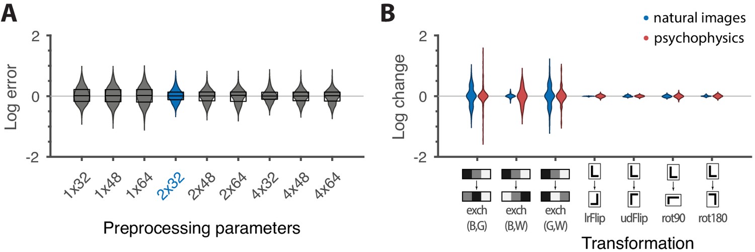
Robustness of results and effects of symmetry transformations.

(A) The difference between the natural logarithms of the measured and predicted thresholds (red crosses and blue dots, respectively, in Figures 4C and 5) is approximately independent of the downsampling ratio $N$ and patch size $R$ used in preprocessing. The labels on the x-axis are in the format $N \times R$ , with the violin plot and label in blue representing the analysis that we focused on in the rest of the paper. Each violin plot in the figure shows a kernel density estimate for the distribution of prediction errors for the 311 second-order single- and mixed-plane threshold measurements available in the psychophysics. The boxes show the 25th and 75th percentiles, and the lines indicate the medians. (B) Change in the natural logarithms of predicted (blue) or measured (red) thresholds following a symmetry transformation. Symmetry transformations that leave the natural image predictions unchanged also leave the psychophysical measurements unchanged. (See text for the special case of the exch(B,W) transformation.) The visualization style is the same as in panel A, except boxes and medians are not shown. The transformations starting with exch correspond to exchanges between gray levels; e.g., exch(B,W) exchanges black and white. lrFlip and udFlip are left-right and up-down geometric flips, respectively, while rot90 and rot180 are geometric rotations by the respective number of degrees (clockwise).

Appendix 5—figure 1

Download asset Open asset

Distribution of prediction errors across specific subsets of thresholds.

Each plot shows kernel-density estimates of the distribution of log prediction errors (defined as difference between log prediction and log measurement) after splitting the data into the subgroups indicated at the top right of each plot. Individual data points are shown on the abscissa. The median log prediction error is shown for each group in the corresponding color. (A) Predictions tend to underestimate thresholds in simple planes and overestimate thresholds in mixed planes ( $p = 0.0014$ , Kolmogorov-Smirnov (K–S) test). As a reminder, the natural-image analysis predicts thresholds only up to a multiplicative factor, which is chosen in a way that makes the mean log prediction error over all second-order thresholds be zero. (B) Predictions tend to have greater error in planes defined by modular sums (such as the simple plane $β_{+ +}$ or the mixed plane $(β_{+ +} [0], β_{\binom{+}{+}} [1])$ ) than in planes defined by modular differences (such as the simple plane $β_{+ -}$ or the mixed plane $(β_{+ -} [1], β_{\binom{+}{-}} [0])$ ) ( $p = 1.8 \cdot 10^{- 4}$ , K-S test). However, thresholds in neither subgroup are systematically over- or under-estimated. (C) There is no significant difference in predictions in on-axis directions (directions parallel to an axis in a simple or mixed coordinate plane), *vs.* all other (off-axis) directions ( $p = 0.56$ , K-S test). (D) Thresholds are more accurately predicted for ‘2-D’ correlations than ‘1-D’ correlations. A mixed plane like $(β_{+ +} [0], β_{+ -} [0])$ involves the same pair of checks in both directions, thus leading to correlations that are in a sense 1-D. In contrast, the mixed plane $(β_{+ +} [1], β_{\binom{+}{-}} [0])$ involves the three checks $A_{1}$ , $A_{2}$ , and $A_{3}$ , leading to 2-D correlations. While the medians of the errors in these two subgroups are similar (KS test $p = 0.25$ ; Wilcoxon rank-sum test $p = 0.96$ , medians 0.042 *vs.* 0.004, respectively), prediction error magnitude is lower for 2-D correlations ( $p = 0.01$ , KS-test on absolute log errors).

Appendix 5—figure 2

Download asset Open asset

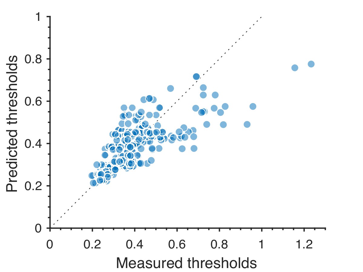
Predictions for large thresholds, corresponding to low-sensitivity directions in texture space, consistently underestimate measured thresholds.

The plot shows the 311 second-order values.

Appendix 6—figure 1

Download asset Open asset

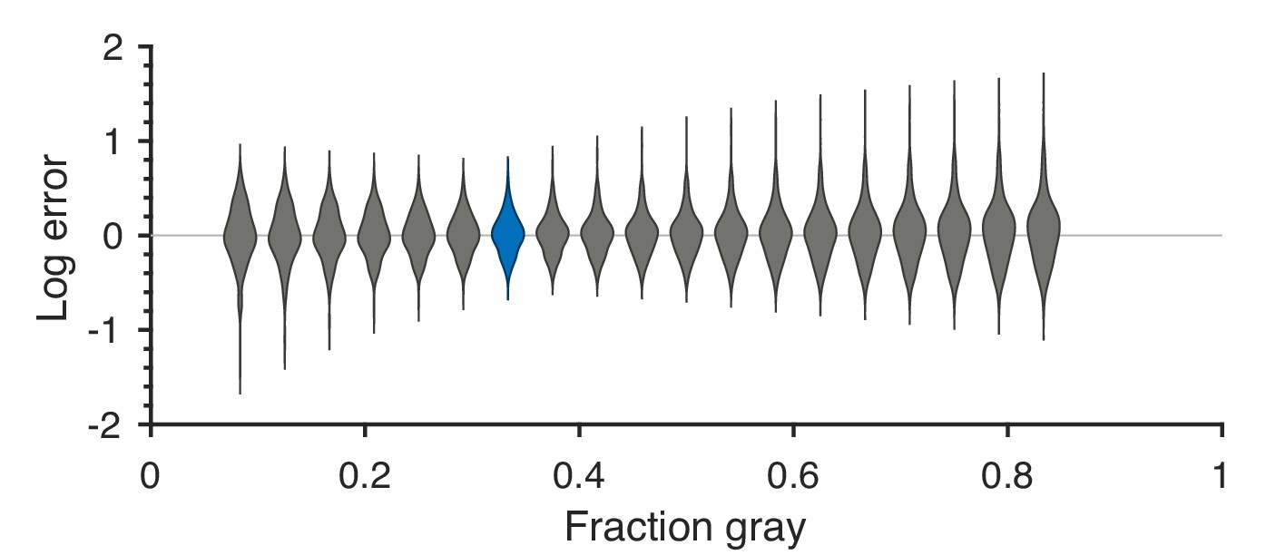
Robustness to changing ternarization thresholds.

We varied the fraction of gray checks in the ternarized natural image patches, while keeping the fractions of black and white checks equal to each other. For each value of the fraction of gray checks, we recalculated the threshold predictions and compared them to the psychophysical measurements. Each violin in the figure shows a kernel density estimate for the distribution of prediction errors (in log space) for the 311 second-order single- and mixed-plane threshold measurements available in the psychophysics. We see that the precise thresholds used for ternarization do not significantly affect the match between natural image predictions and psychophysics. The lowest error is close to the value 1/3 which corresponds to equal fractions of black, gray, and white checks, and is the one used in the main text. The corresponding violin is highlighted in blue in the figure.

Appendix 6—figure 2

Download asset Open asset

Natural image predictions (blue dots) for second-order planes when using the van Hateren image database (van Hateren and van der Schaaf, 1998).

The psychophysics measurements are also shown, in red crosses. The notations are as described in the main text (Figure 5).

Appendix 6—figure 3

Download asset Open asset

Psychophysical thresholds in the second-order planes shown for different subjects.

Depending on the plane, measurements were made in 2–5 subjects in each texture direction. The notations are as in the main text (Figure 5).

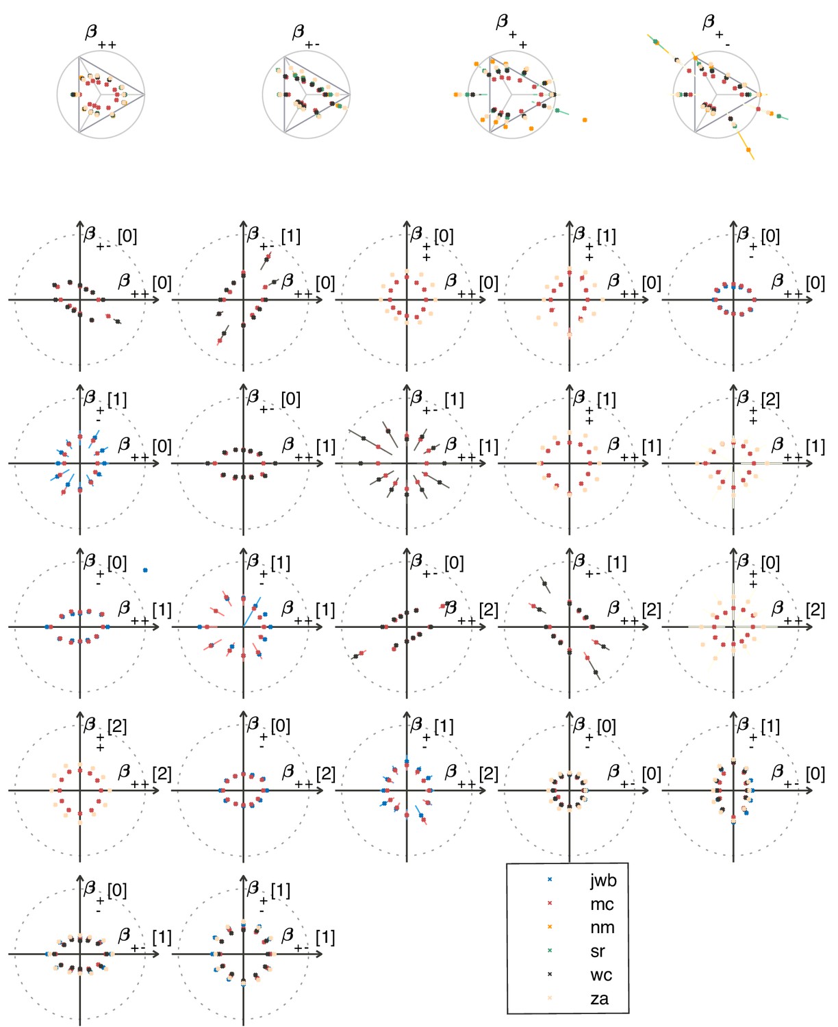
Appendix 6—figure 4

Download asset Open asset

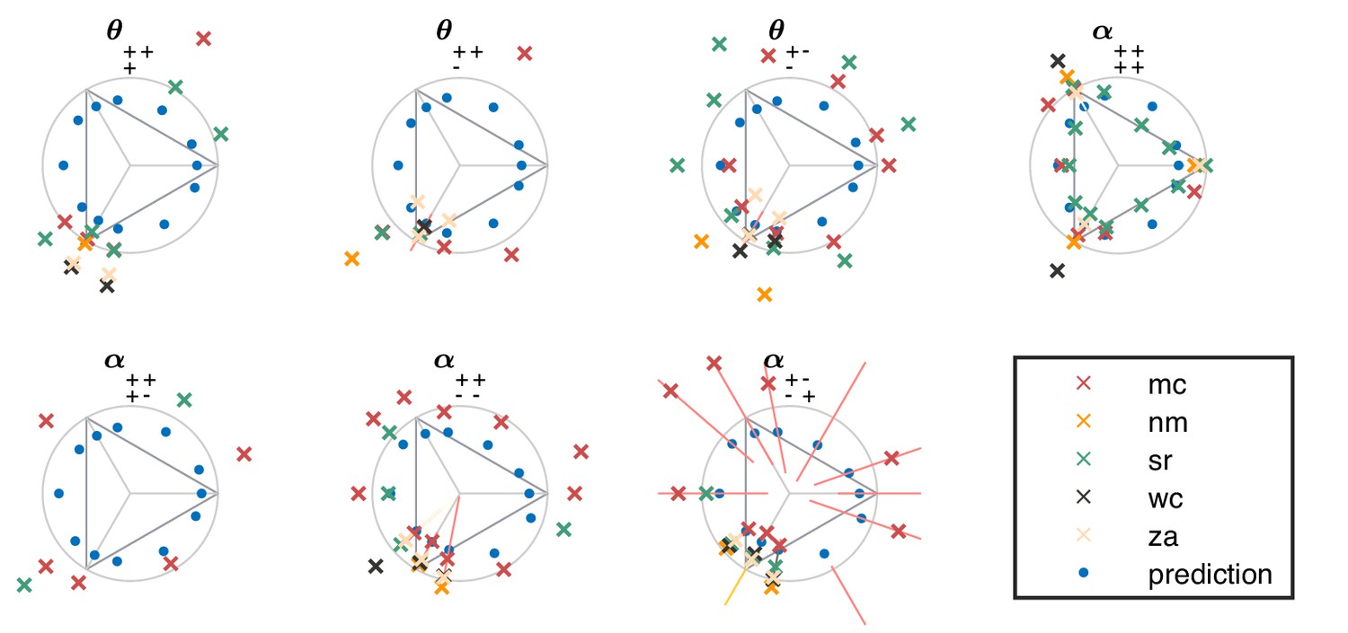
Psychophysical thresholds in higher-order planes for individual subjects (crosses).

The natural image predictions are also shown, in blue dots. The notations are as in the main text (Figure 4). in many directions, performance did not sufficiently exceed chance to allow for a reliable determination of threshold; in these cases, data points are omitted.

Tables

Appendix 4—table 1

Results from statistical tests comparing the match between measured and predicted thresholds to chance.

The left column gives the preprocessing parameters $N$ (the downsampling factor) and $R$ (the patch size) in the format $N \times R$ . For each of the permutation tests, a $p$ -value and the shortest interval containing 95% of the $D$ values obtained in 10,000 samples is given (the 95% highest-density interval, or HDI). Similarly, for the exponent estimation, we include the shortest interval containing 95% of the posterior density for each of the two model parameters (the 95% highest posterior-density interval, or HPDI).

		1. Permutation #1		2. Permutation #2		3. exponent estimation
(l)3-8			D		D	η	σ
$N \times R$	$D_{actual}$	p	[95% HDI]	p	[95% HDI]	[95% HPDI]	[95% HPDI]
$1 \times 32$	0.20	<10⁻⁴	$[0.26, 0.33]$	0.0041	$[0.21, 0.27]$	$[0.58, 0.75]$	$[0.22, 0.26]$
$1 \times 48$	0.20	<10⁻⁴	$[0.28, 0.35]$	0.0020	$[0.22, 0.29]$	$[0.52, 0.67]$	$[0.22, 0.25]$
$1 \times 64$	0.21	<10⁻⁴	$[0.29, 0.37]$	0.0010	$[0.23, 0.31]$	$[0.50, 0.63]$	$[0.21, 0.25]$
$2 \times 32$	0.13	<10⁻⁴	$[0.24, 0.31]$	<10⁻⁴	$[0.16, 0.22]$	$[0.81, 0.98]$	$[0.18, 0.22]$
$2 \times 48$	0.15	<10⁻⁴	$[0.26, 0.33]$	<10⁻⁴	$[0.18, 0.23]$	$[0.71, 0.85]$	$[0.18, 0.21]$
$2 \times 64$	0.16	<10⁻⁴	$[0.27, 0.34]$	<10⁻⁴	$[0.18, 0.24]$	$[0.66, 0.79]$	$[0.18, 0.22]$
$4 \times 32$	0.12	<10⁻⁴	$[0.24, 0.30]$	<10⁻⁴	$[0.15, 0.20]$	$[0.87, 1.04]$	$[0.18, 0.22]$
$4 \times 48$	0.14	<10⁻⁴	$[0.26, 0.33]$	0.0003	$[0.16, 0.22]$	$[0.74, 0.89]$	$[0.18, 0.21]$
$4 \times 64$	0.15	<10⁻⁴	$[0.26, 0.34]$	0.0002	$[0.16, 0.23]$	$[0.69, 0.83]$	$[0.18, 0.21]$

Appendix 6—table 1

Results from statistical tests comparing the match between measured and predicted thresholds to chance when using the van Hateren natural image database (van Hateren and van der Schaaf, 1998).

		1. Permutation #1		2. Permutation #2		3. exponent estimation
(l)3-8			D		D	η	σ
$N \times R$	$D_{actual}$	p	[95% HDI]	p	[95% HDI]	[95% HPDI]	[95% HPDI]
$1 \times 32$	0.22	<10⁻⁴	$[0.27, 0.34]$	0.0081	$[0.23, 0.31]$	$[0.45, 0.63]$	$[0.24, 0.28]$
$1 \times 48$	0.23	<10⁻⁴	$[0.30, 0.37]$	0.0013	$[0.26, 0.34]$	$[0.41, 0.57]$	$[0.24, 0.28]$
$1 \times 64$	0.24	<10⁻⁴	$[0.30, 0.38]$	0.0020	$[0.26, 0.34]$	$[0.40, 0.54]$	$[0.24, 0.27]$
$2 \times 32$	0.16	<10⁻⁴	$[0.26, 0.32]$	0.0001	$[0.19, 0.25]$	$[0.67, 0.84]$	$[0.21, 0.24]$
$2 \times 48$	0.18	<10⁻⁴	$[0.27, 0.34]$	0.0003	$[0.20, 0.27]$	$[0.58, 0.73]$	$[0.21, 0.24]$
$2 \times 64$	0.19	<10⁻⁴	$[0.28, 0.36]$	0.0002	$[0.21, 0.28]$	$[0.54, 0.67]$	$[0.21, 0.24]$
$4 \times 32$	0.14	<10⁻⁴	$[0.25, 0.32]$	0.0002	$[0.17, 0.24]$	$[0.73, 0.90]$	$[0.20, 0.23]$
$4 \times 48$	0.15	<10⁻⁴	$[0.27, 0.34]$	<10⁻⁴	$[0.18, 0.26]$	$[0.64, 0.78]$	$[0.19, 0.23]$
$4 \times 64$	0.16	<10⁻⁴	$[0.28, 0.36]$	<10⁻⁴	$[0.20, 0.26]$	$[0.59, 0.73]$	$[0.19, 0.23]$

Additional files

Transparent reporting form: https://cdn.elifesciences.org/articles/54347/elife-54347-transrepform-v2.docx
Download elife-54347-transrepform-v2.docx

Download links

A two-part list of links to download the article, or parts of the article, in various formats.

Downloads (link to download the article as PDF)

Article PDF

Open citations (links to open the citations from this article in various online reference manager services)

Mendeley

Cite this article (links to download the citations from this article in formats compatible with various reference manager tools)

Tiberiu Tesileanu
Mary M Conte
John J Briguglio
Ann M Hermundstad
Jonathan D Victor
Vijay Balasubramanian

(2020)

Efficient coding of natural scene statistics predicts discrimination thresholds for grayscale textures

eLife 9:e54347.

https://doi.org/10.7554/eLife.54347

Share this article

Cite this article

Ternary texture analysis.

Examples of textures from all the mixed planes for which psychophysics data are available.

Preprocessing of natural images.

Experimental setup and results in second-order simple planes.

The match between measured (red crosses and error bars) and predicted (blue dots) thresholds in 22 mixed planes.

Robustness of results and effects of symmetry transformations.

Distribution of prediction errors across specific subsets of thresholds.

Predictions for large thresholds, corresponding to low-sensitivity directions in texture space, consistently underestimate measured thresholds.

Robustness to changing ternarization thresholds.

Natural image predictions (blue dots) for second-order planes when using the van Hateren image database (van Hateren and van der Schaaf, 1998).

Psychophysical thresholds in the second-order planes shown for different subjects.

Psychophysical thresholds in higher-order planes for individual subjects (crosses).

Results from statistical tests comparing the match between measured and predicted thresholds to chance.

Results from statistical tests comparing the match between measured and predicted thresholds to chance when using the van Hateren natural image database (van Hateren and van der Schaaf, 1998).

Transparent reporting form

Downloads (link to download the article as PDF)

Open citations (links to open the citations from this article in various online reference manager services)

Cite this article (links to download the citations from this article in formats compatible with various reference manager tools)