A Matlab-based toolbox for characterizing behavior of rodents engaged in string-pulling
- Canadian Centre for Behavioural Neuroscience, University of Lethbridge, Canada
Figures
Figure 1
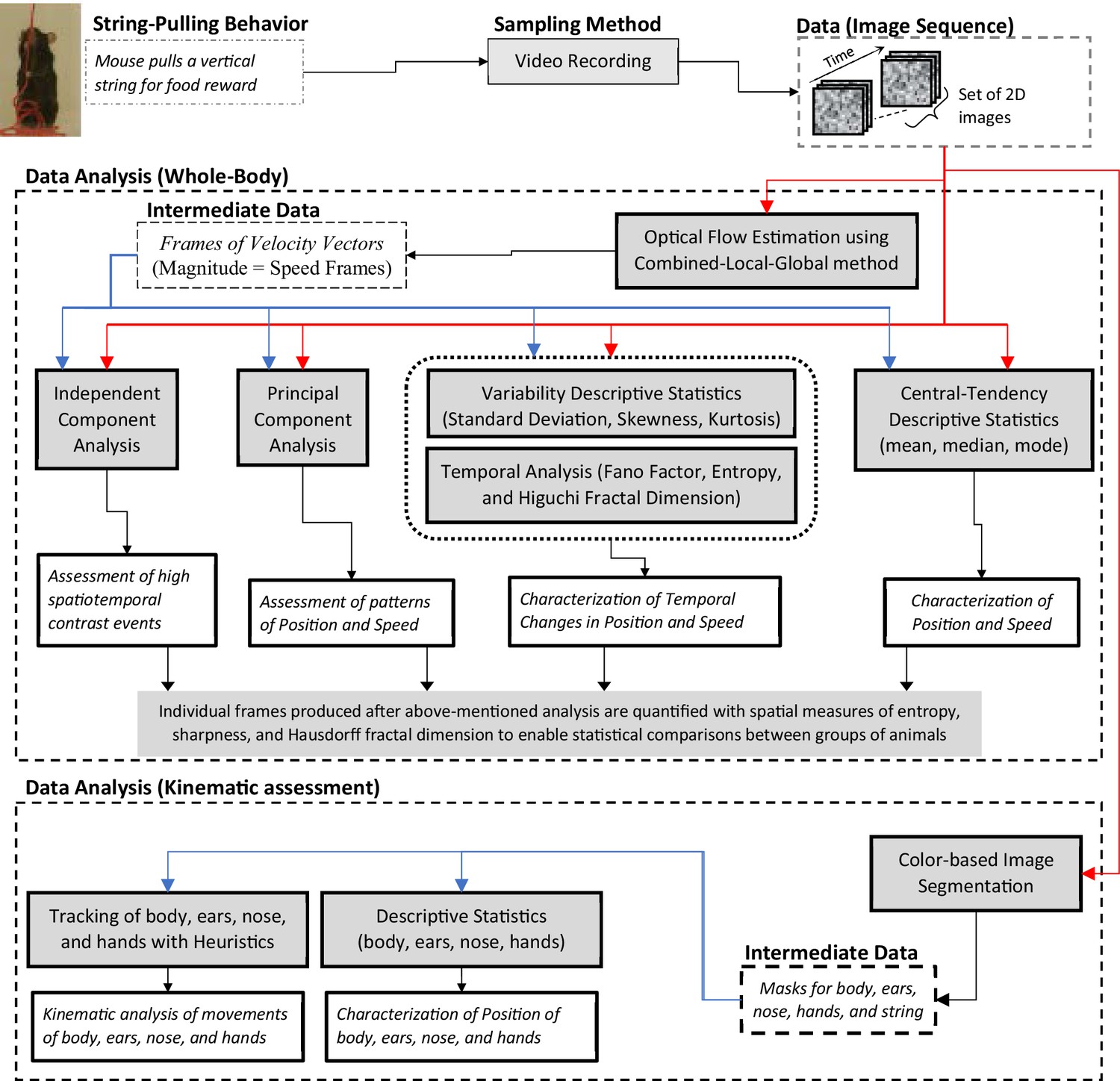
String-pulling video analysis framework.
Characterization of whole-body position and speed and their temporal variability is assessed with descriptive statistics, Fano factor, entropy, and Higuchi fractal dimension. Speed is estimated with optical flow estimation. Principal and independent component analysis of frames of image sequence and speed frames provide overall assessment of position and speed patterns. Measures of spatial entropy, sharpness, and Hausdorff fractal dimension on frames obtained in earlier steps are used to statistically compare global position and motion patterns of groups of animals. For fine kinematic assessment of the motion of body, ears, nose, and hands, they are tracked using image segmentation and heuristic algorithms. Shaded boxes represent methods.
Figure 2

Characterization of whole-body position using central-tendency descriptive statistics.
(A) Representative subset of image frames of a string-pulling epoch of a Black mouse. (B) Central-tendency descriptive statistics: mean, median, and mode of string-pulling image sequence for a Black mouse. Mean, median, and mode frames represent average to most frequent position of mouse. Shown below each frame are the respective values of measures of spatial entropy, sharpness, and Hausdorff fractal dimension separated by hyphens. The black line in the mean frame shows the boundary of a mask generated by selecting all pixels with values above the average value of the mean frame. (C) and (D) same as (A) and (B) respectively but for a White mouse. Descriptive statistics of representative Black mouse show sitting as most frequent posture while that of the White mouse is upright standing. (E) Mean ± SEM spatial entropy, sharpness, and Hausdorff fractal dimension shown for frames of descriptive statistics from 5 Black and 5 White mice.
Figure 3
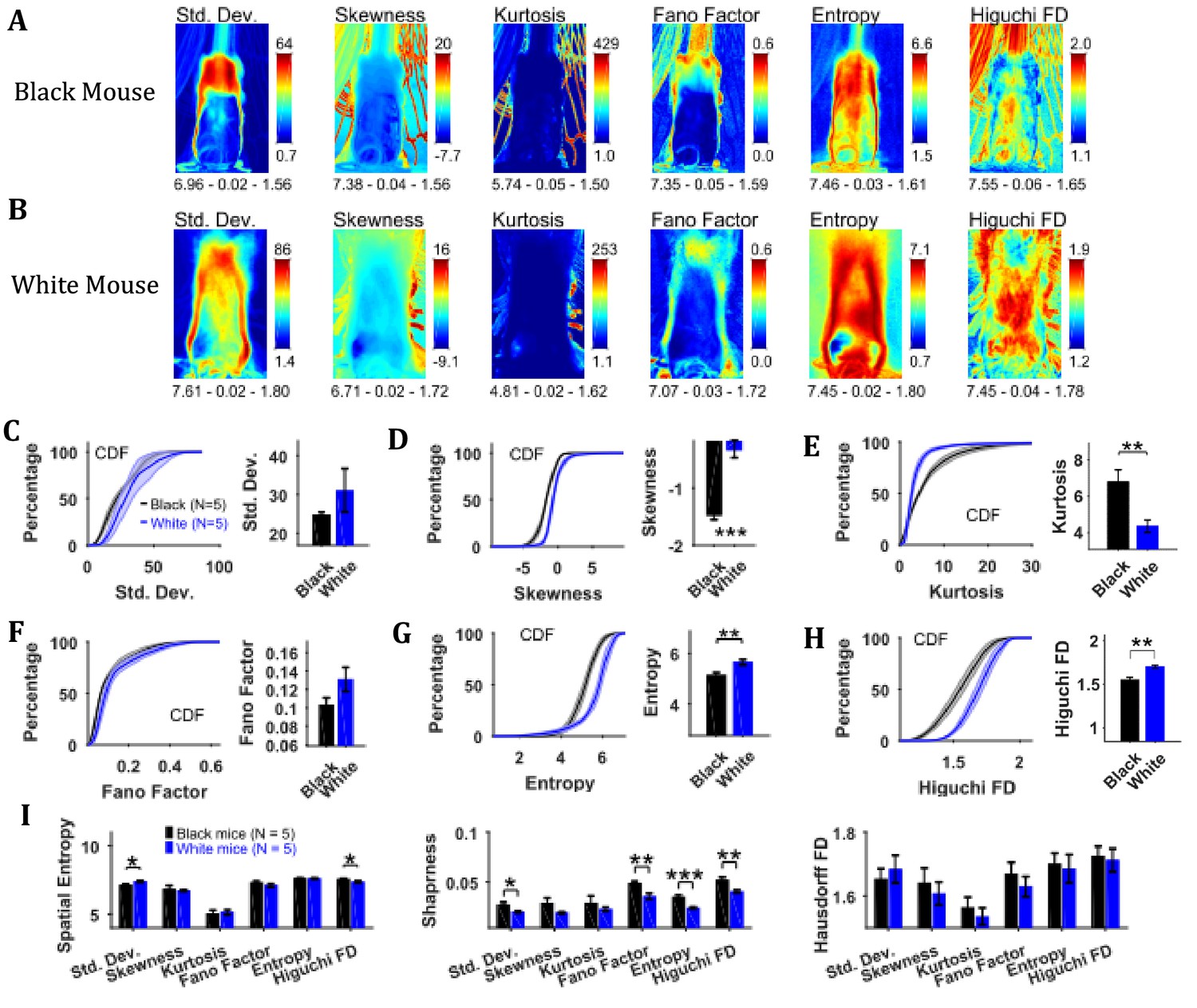
Characterization of changes in position with variability descriptive statistics, Fano factor, entropy, and Higuchi fractal dimension.
(A) Representative variability descriptive statistics – standard deviation (Std. Dev.), skewness, and kurtosis, Fano factor, Entropy, and Higuchi fractal dimension of string-pulling image sequence of a Black mouse. Standard deviation depicts summary of spatial variation over time (mouse posture from sitting to standing). Skewness and kurtosis capture regions of rare events around the mouse body such as position of string. Shown below each frame are the respective values of spatial entropy (SE), sharpness (S), and Hausdorff fractal dimension (HFD) separated with a hyphen. (B) same as (A) but for White mouse. The White mouse has greater yaw and pitch head motion as seen in the standard deviation. (C) Mean ± SEM cumulative distribution function (CDF) of the standard deviation values within a mask obtained for each individual mouse from their respective mean frames. For the representative Black and White mice, outline of these masks is shown in Figure 2B and D, respectively. (D–H) Same as (C) but for other parameters. (I) Mean ± SEM SE, S, and HFD shown for frames of parameters mentioned above.
Figure 4
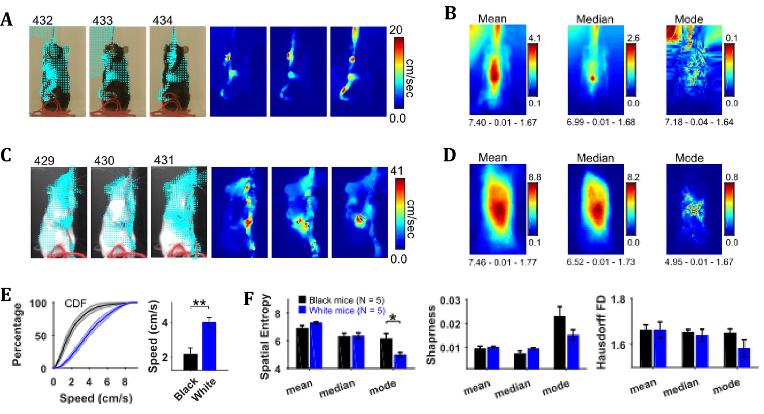
Characterization of speed with central-tendency descriptive statistics reveals White mice have larger speeds compared to Black mice.
(A) Output of the optical flow analysis overlayed on three representative image frames. Velocity vector is shown for every fifth pixel (along both dimensions). For a pixel, the magnitude of the velocity vector shows instantaneous speed (cm/s). For the same image frames, respective speed frames are shown on the right. (B) Descriptive statistics of the speed frames. Shown below each frame are the respective values of spatial entropy (SE), sharpness (S), and Hausdorff fractal dimension (HFD) separated with a hyphen. The unit of color code is cm/sec. (C) and (D) same as (A) and (B) respectively but for White mouse. (E) Average cumulative distributions of speeds from the mean speed frames of Black (N = 5) and White (N = 5) mice. Shaded regions show SEM. Bar graph show Mean ± SEM over animals of mean speeds. (F) Mean ± SEM SE, S, and HFD shown for frames of descriptive statistics from 5 Black and 5 White mice.
Figure 5
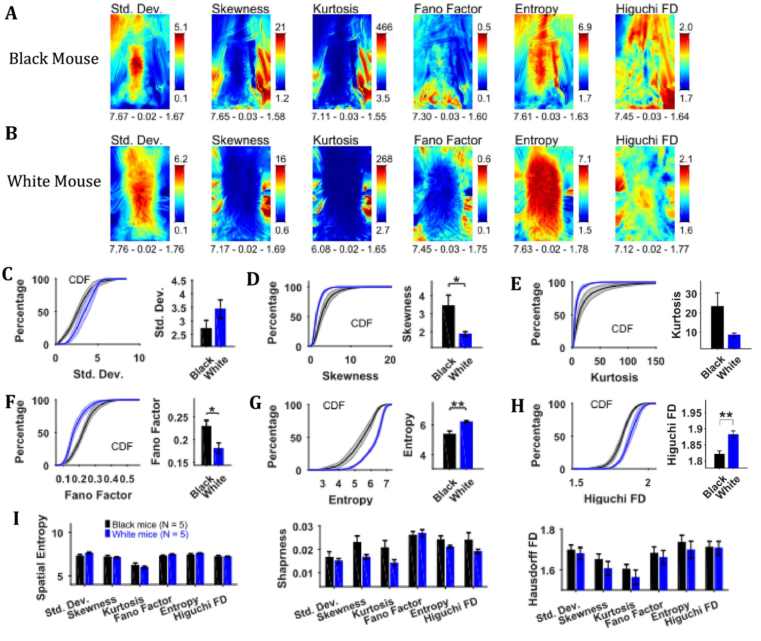
Characterization of changes in speed with variability descriptive statistics, Fano factor, entropy, and Higuchi fractal dimension.
(A) Representative variability descriptive statistics – standard deviation (Std. Dev.), skewness, and kurtosis, Fano factor, Entropy, and Higuchi fractal dimension of speed frames of a Black Mouse. Shown below each frame are the respective values of spatial entropy (SE), sharpness (S), and Hausdorff fractal dimension (HFD) separated with a hyphen. (B) Same as (A) but for a White mouse. (C) Mean ± SEM cumulative distributions (CDF) of standard deviation values within a mask obtained for each individual mouse from their respective mean frames. For the representative Black and White mice, outline of these masks is shown in Figure 2B and D, respectively. (D–H) Same as (C) but for other parameters. (I) Mean ± SEM SE, S, and HFD shown for frames of parameters mentioned above.
Figure 6

Principal component analysis of image sequence and speed frames for assessment of patterns of positions and speeds.
(A) The first four principal components (PC) of the image sequence of the representative Black mouse. The number in parentheses indicates the value of explained variance. Shown below each frame are the respective values of spatial entropy (SE), sharpness (S), and Hausdorff fractal dimension (HFD) separated with a hyphen. (B) First four PCs of speed frames for the Black mouse. (C) and (D) same as (A) and (B) respectively but for the representative White mouse. (E) Mean ± SEM values of explained variance (Var.), SE, S, and HFD for PC1 of positions and speeds.
Figure 7
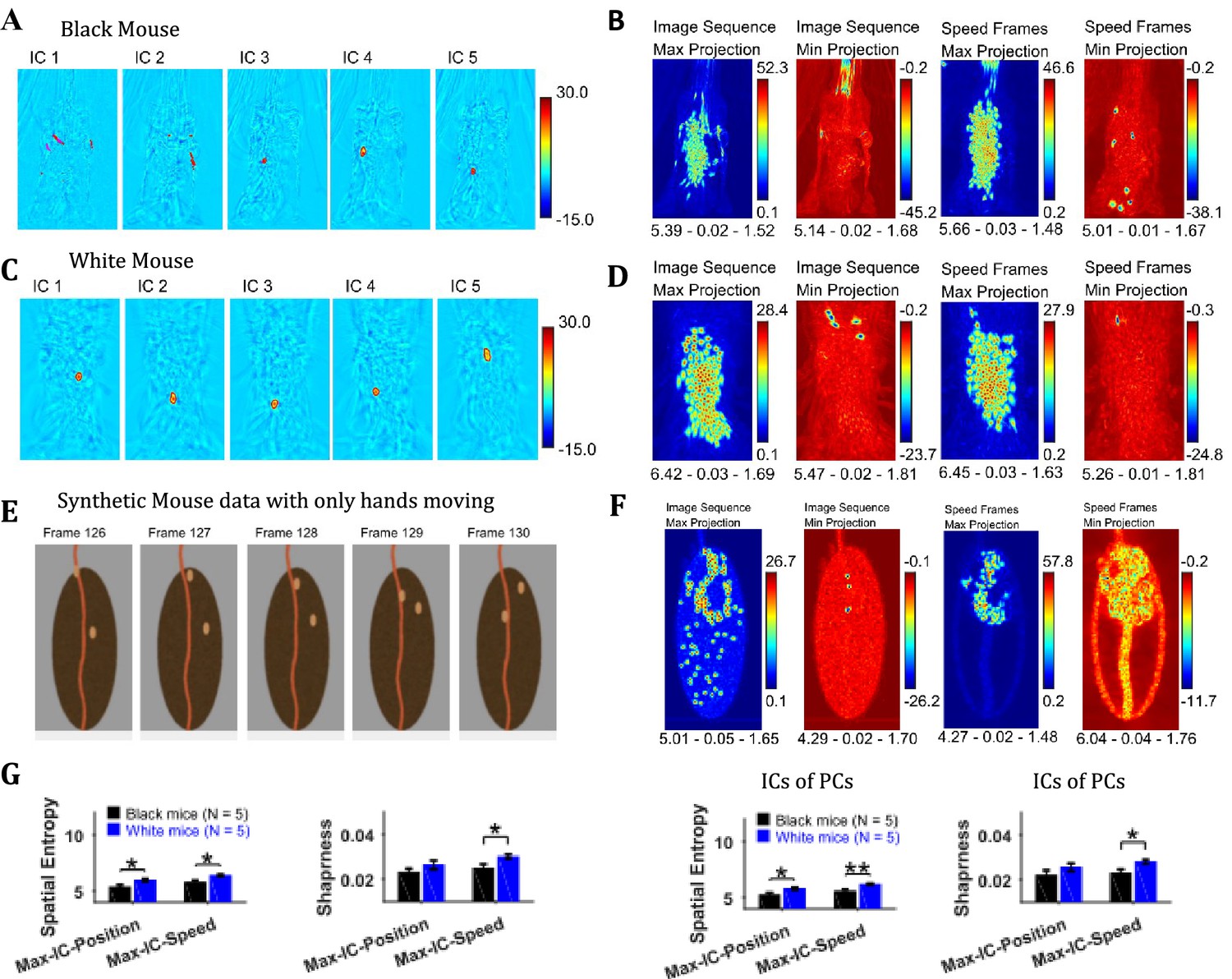
Independent component analysis captures regions with high spatiotemporal contrast.
(A) Representative independent components for Black mouse. Individual independent components mostly represent snapshots of position of the hands and strings, as they are most dynamic in the image sequence. (B) Maximum (Max) and minimum (Min) value projections of all independent components of image sequence and speed frames. Max and Min projections grossly represent locations of sudden changes happening in an image sequence for example, hand appearing or disappearing at a new location. Shown below each frame are the respective values of spatial entropy, sharpness, and Hausdorff fractal dimension separated with a hyphen. (C) and (D) similar to (A) and (B) respectively but for White mouse. (E) Representative image frames of synthetic mouse data in which only hands moved. (F) Similar to (B) but for synthetic data. (G) Mean ± SEM of spatial entropy and sharpness of Max projections of ICs for image sequence, speed frames and their respective PCs.
Figure 8
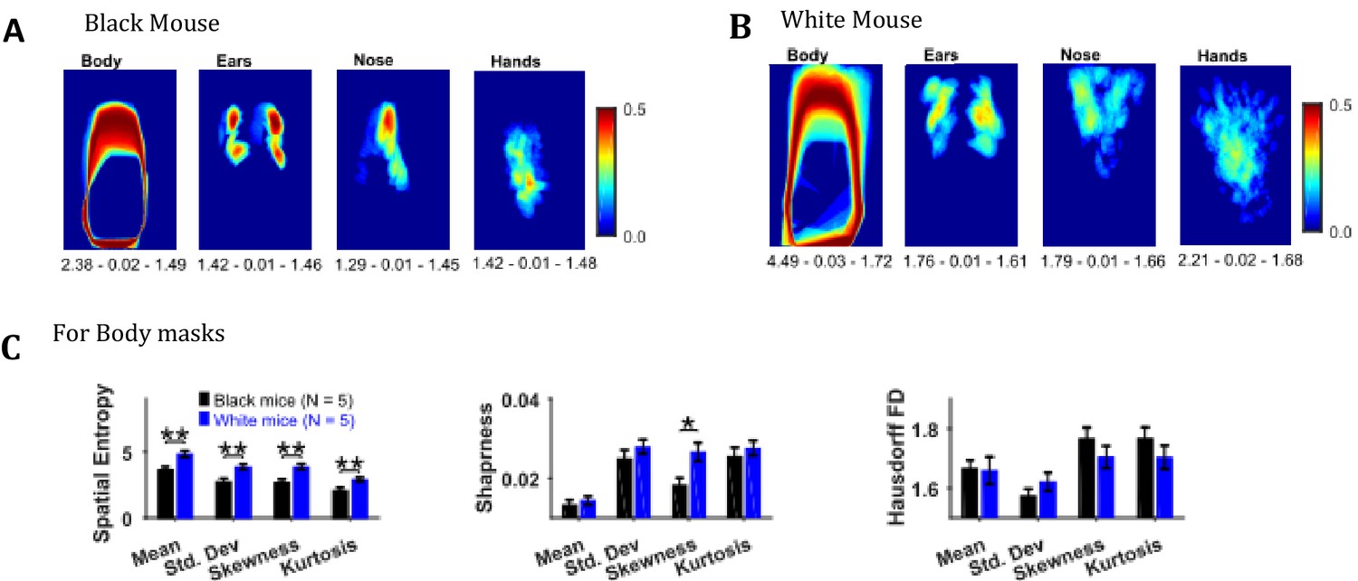
Image segmentation based on object colors for finding object masks and gross assessment from descriptive statistics of masks.
(A–B) Standard deviation of the masks image sequence of body, ears, nose, and hands for overall assessment of respective motion patterns of Black and White mice, respectively. Shown below each frame are the respective values of spatial entropy (SE), sharpness (S), and Hausdorff fractal dimension (HFD) separated with a hyphen. (C) Mean ± SEM SE, S, and HFD shown for Body masks.
Figure 9 with 1 supplement
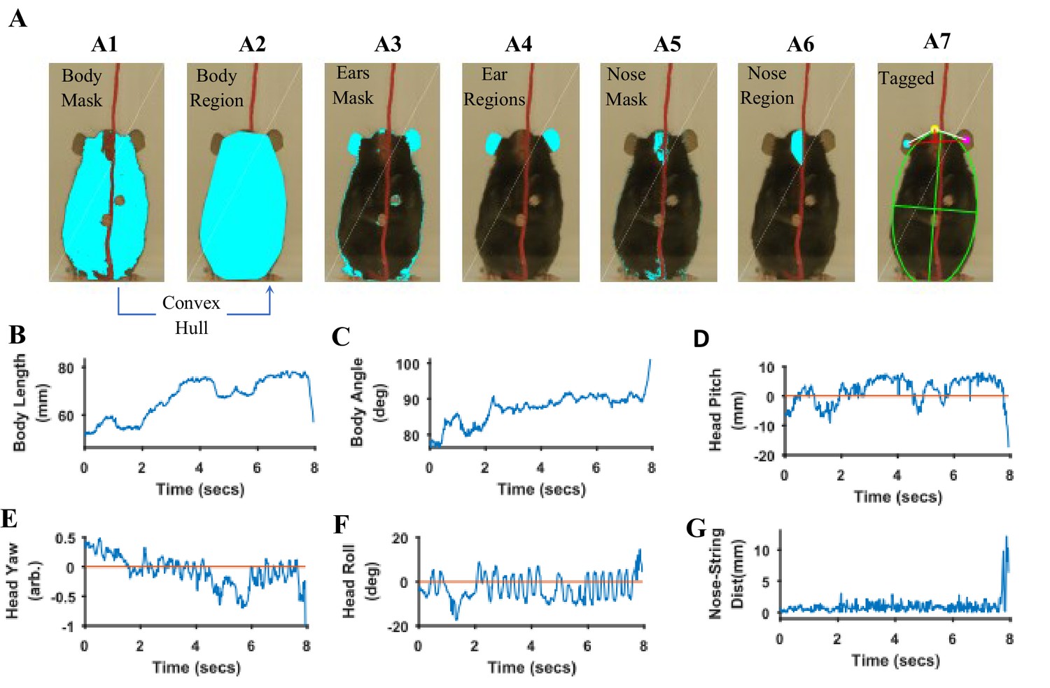
Quantification of body and head posture.
(A) Tagging of body, ears, and nose. From masks found with fur color (A1), body region (A2) is identified and fitted with an ellipse (A7, green). From the ears’ mask (A3), ear regions are identified by using body centroid position found earlier (A4, cyan and magenta dots in A7). Nose mask (A5) is used to identify the nose region (A6), which is fitted with an ellipse to identify nose position (A7, yellow dot). (B) Body length vs time. Body length is the length of major axis of the body fitted ellipse. (C) Body Angle vs time. Body angle is that of the major axis of the body fitted ellipse from horizontal. (D) Head Pitch vs time. Head pitch is estimated as the perpendicular distance between the nose and a straight line joining the ears (small red line in A7). Positive and negative values correspond to the nose above or below the line respectively. (E) Head Yaw vs time. Head yaw is estimated by finding the log of the ratio of distance of right ear from the nose to the distance of left ear from the nose (ratio of lengths of White lines in A7). A value of 0 indicates 0 yaw angle. (F) Head Roll Angle vs time. Head roll is the angle of the line joining ear centroids from horizontal using the right ear as the origin. (G). Shortest distance of the nose from the string vs time.
Figure 9—figure supplement 1
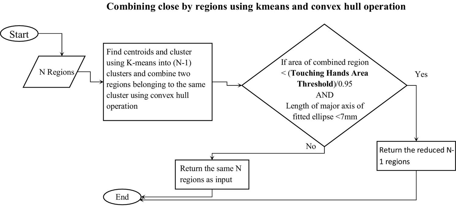
Algorithm to reduce the number of regions by spatial clustering.
Close by regions are combined provided that the combined region’s area is less than the threshold and the length of the major axis of fitted ellipse is less than 7 mm. For ears and nose, only the length of major axis of fitted ellipse should be less than 9 and 8 mm respectively.
Figure 10 with 1 supplement
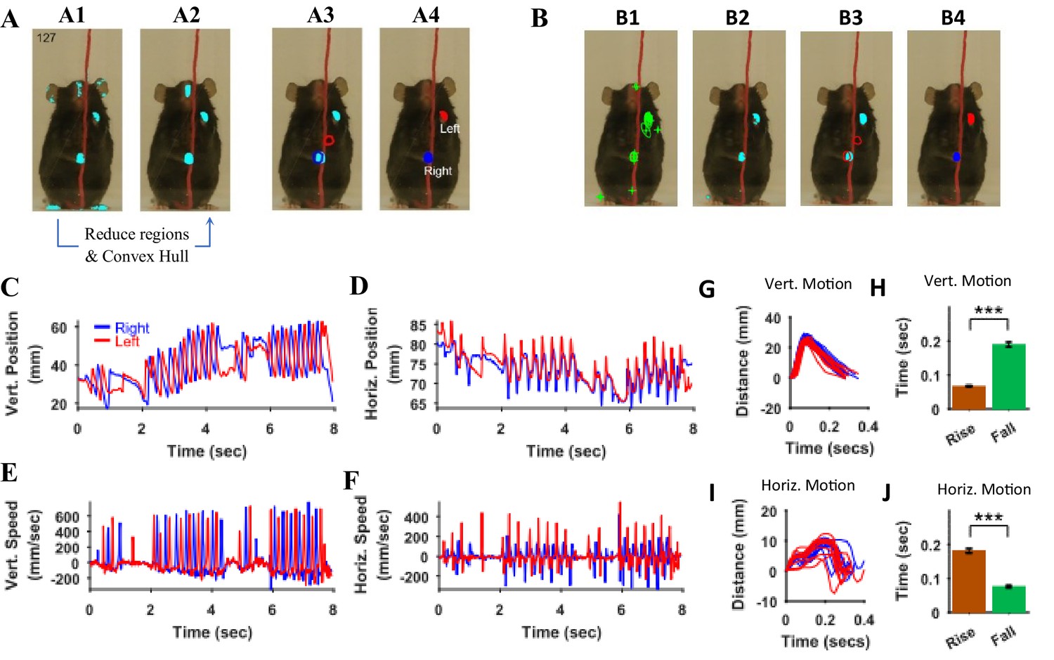
Identification of hands and kinematic measures.
(A) Representative frame (127) with overlayed regions in hand masks (A1). Regions in A1 are reduced to find regions that would most likely represent the hands (A2). Note that it includes a region in the nose area. Using the position of hands in the previous frame (blue and red outlines in A3), the hands are identified in the current frame (A4). (B) same as in A but masks are first found by identifying maximally stable extremal regions in the original image (B1). (C), (D) Vertical (Vert) and Horizontal (Horz) positions vs time of right (blue) and left (red) hands, respectively. Positions are measured from the lower left corner of frame as the origin. Where horizontal movements are synchronized, vertical movements of right and left hands are alternating. (E), (F) Vertical and horizontal speed vs time of right and left hands. Maximum vertical speed is about three times larger than maximum horizontal speed. (G) Distance vs. time for vertical motion plotted from all reach cycles (lift-advance-grasp-pull-push-release). Red for left hand and blue for right hand motion. (H) Mean ± SEM rise and fall times for vertical motion reaches. (I) and (J) similar to G) and H) respectively but for horizontal motion. Also see Video 1 and Video 2.
Figure 10—figure supplement 1
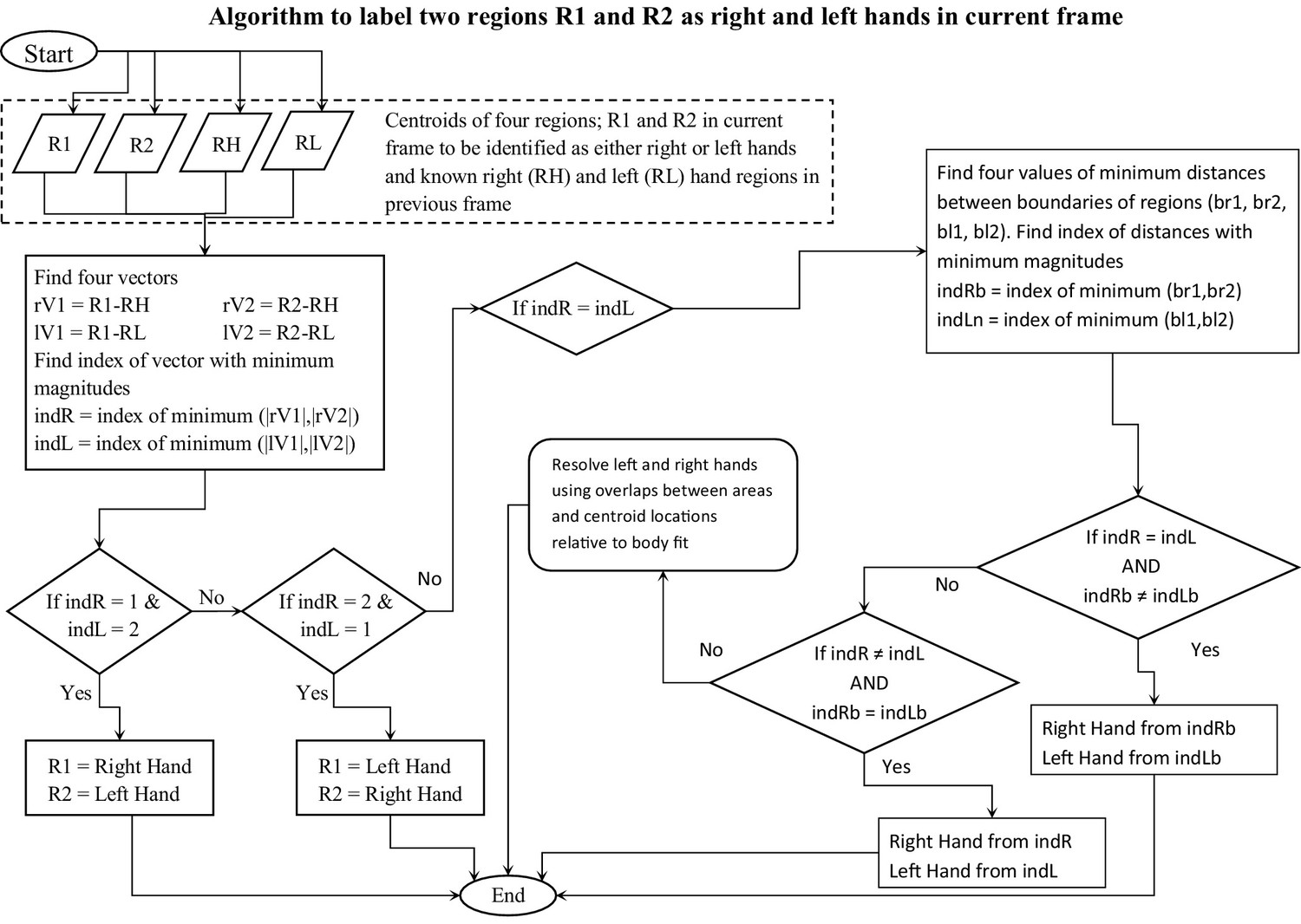
Algorithm to label right- and left-hand regions from two unlabeled regions.
The algorithm primarily uses distances of unlabelled regions from the right- and left-hand regions in the previous frame to label them as right and left hands.
Figure 11 with 1 supplement
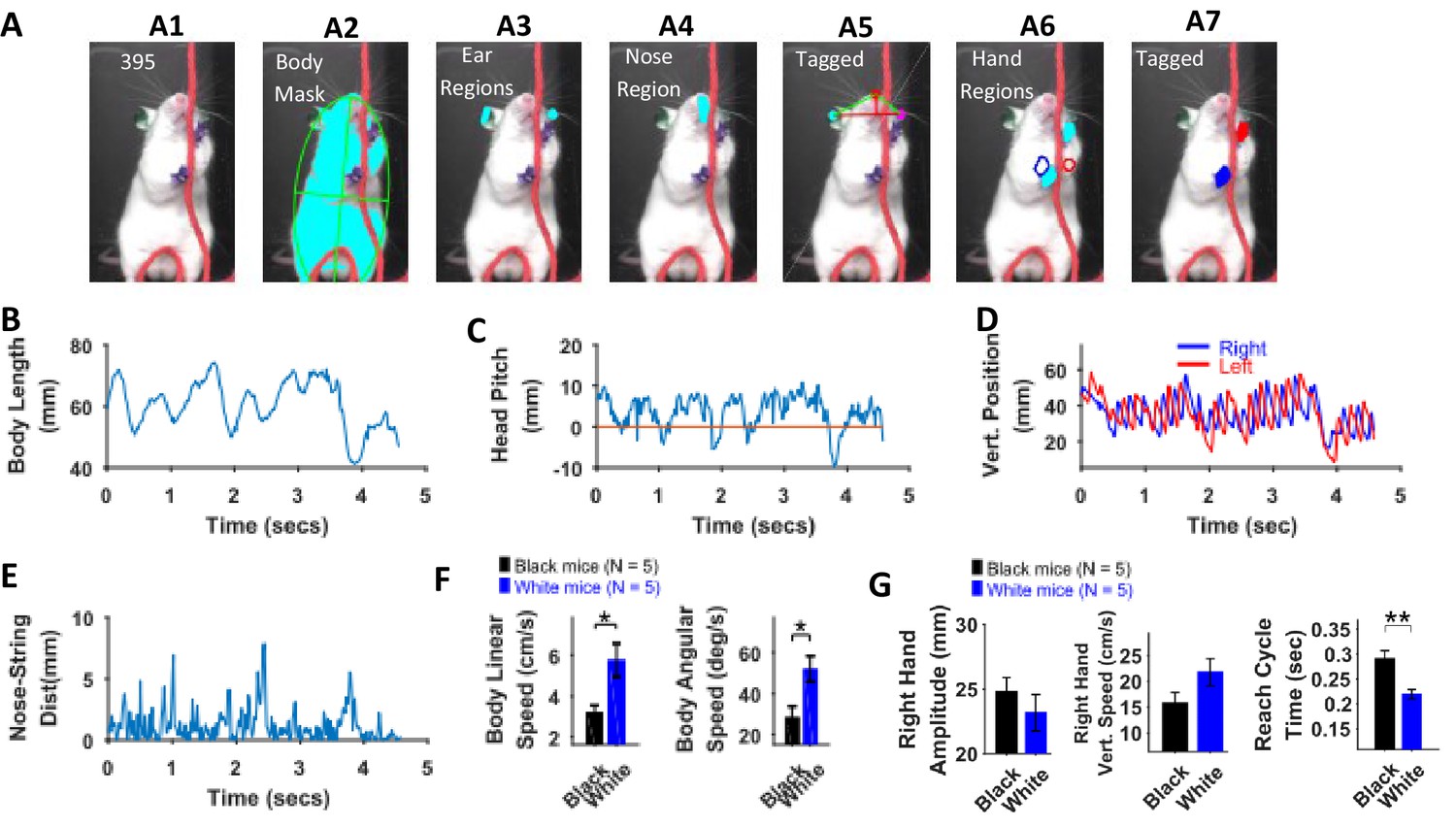
Identification of body parts and quantification of kinematic measures in White mice.
(A) Procedure for tagging of body, ears, nose, and hands was like that used for Black mice except that the ears and hands were colored green and blue respectively. From masks found using fur color (A2), the body region is identified and fitted with an ellipse. Ear and nose regions (A3 and A4, respectively) are identified and used to measure head posture (A5). Hand regions (A6) are identified based on the position of the hands in the previous frame (A6, red and blue boundaries), the position of the hands in the current frame are identified (A7). (B) Body length vs time. (C) Head Pitch vs time. In frames where both ears are not visible, y-distance between nose and ear is measured as head pitch. D) Vertical position of the hands (from bottom of frame) vs time. (E) Shortest distance of the nose from the string vs time. (F) Mean ± SEM of body linear and angular speeds from five Black and five White mice. (G) Mean ± SEM amplitude, vertical speed, and time period of reach cycle of right hand.
Figure 11—figure supplement 1
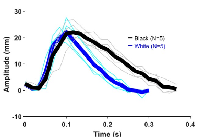
Temporal profiling of reach cycle for black and white mice with Dynamic Time Warping.
Light gray and light blue lines indicate time-warped average reach cycles for individual Black and White mice respectively. Darker lines (black and blue) indicate time-warped group average reach cycles. ‘Time-warped average reach cycle’ for each animal was found by the following steps: (1) individual reach cycles were zero padded to make their lengths equal, (2) average reach cycle was obtained from zero padded cycles, (3) time warping of original cycles was done with average reach cycle obtained in step two using Matlab’s ‘dtw’ function, (4) averaging of individually time-warped reach cycles obtained in previous step provided time-warped average reach cycle for an animal (shown by light gray and light blue lines). By following similar steps, time-warped group average reach cycle was found (darker lines, black and blue).
Figure 12
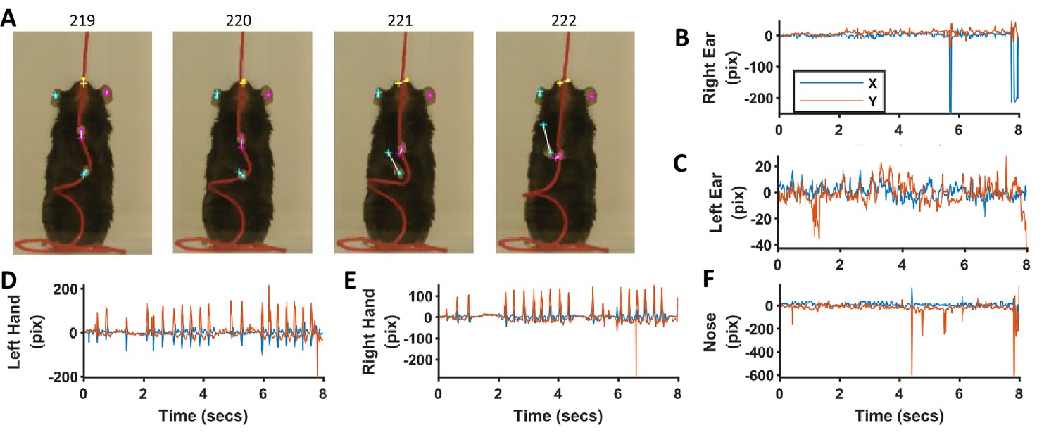
Comparison of identification of ears, nose, and hands with heuristic algorithms and machine-learning-based neural networks.
(A) Representative frames highlighting the differences in position of ears, nose, and hands identified with the two methods. Dots for heuristics and plus for neural networks. (B–F) Differences in x and y coordinates of ears, nose, and hands identified with the two methods.
Figure 13
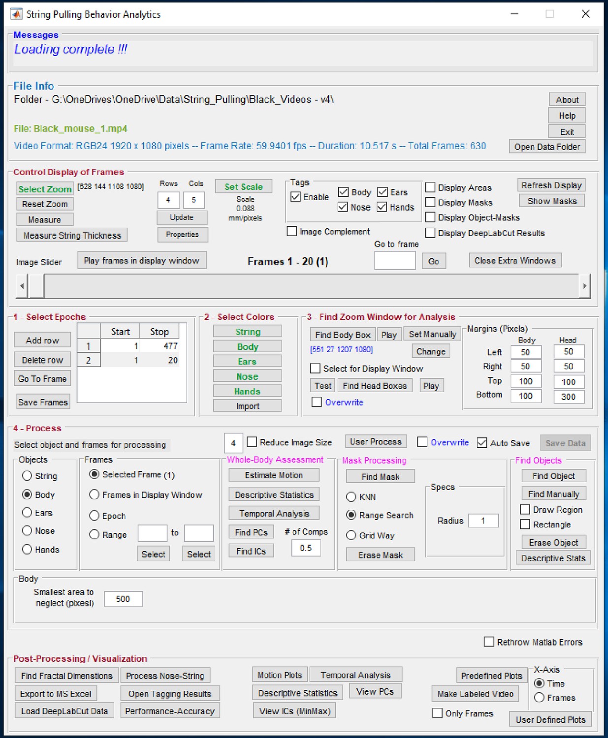
Graphical user interface of the toolbox.
Individual steps for processing data are separated into panel blocks. The video frames can be viewed in the display window using the ‘Control Display of Frames’ panel. Step 0, the user has to define a zoom window for digital magnification of the video and scale for finding pixels/mm. Step 1, the user specifies epochs in which the mouse pulls the string. Step 2, the user defines colors. Step 3, the user finds zoom window, a sub region of the frames for which masks are calculated. Step 4, the user processes the epoch for whole-body analysis through ‘Whole-Body Assessment’ panel and also finds masks and later objects of interest. Finally, the user can generate plots using the ‘Post-Processing’ panel.
Figure 14 with 1 supplement
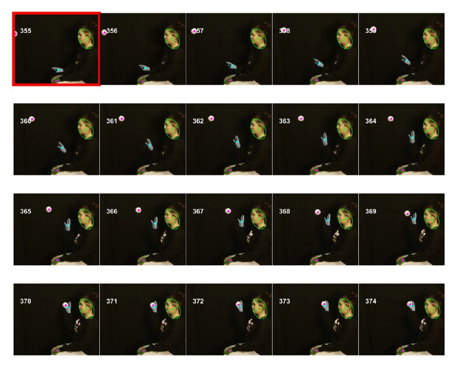
General applicability of the software for tracking objects shown in a video of a human catching and throwing a ball.
Figure 14—figure supplement 1
General applicability of the software for tracking objects shown in a video of a tail-clasped mouse where hind paws and body are tracked.
Figure 15 with 2 supplements
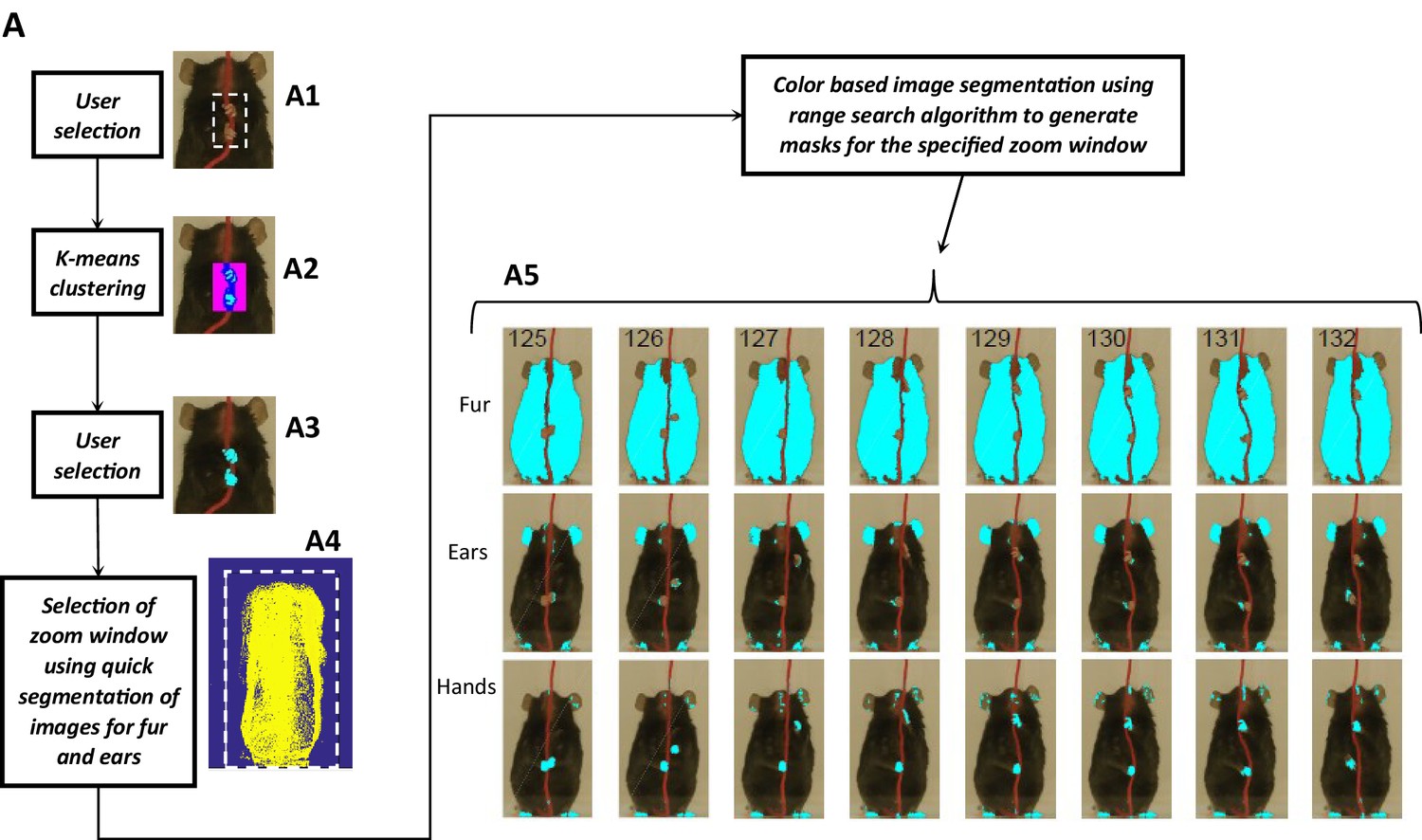
Image segmentation based on object colors for finding object masks and gross assessment from descriptive statistics of masks.
(A) Color definitions in original frames are semi-automatically made with the user’s assistance for fur, ears, nose, hands, and string. The user first selects a rectangular region around the object of interest (A1). K-means clustering is then applied to segregate different colors within the selected region (A2). The user then selects a color that corresponds to the object of interest (A3, example shown for selecting color for the hands). Using color selections for the fur and ears, quick segmentation is used to identify the fur and ears in every frame in an epoch of interest and projected onto a single frame after edge detection (A4). A rectangular window around the blob is drawn to define a sub region of frames for which masks are then found (A5, representative masks). The determination of rectangular window can also be done automatically and modified later if required. Note that masks are not always clean and include regions other than objects of interest for example, hand masks include regions identified in ears and feet because of color similarity.
Figure 15—figure supplement 1
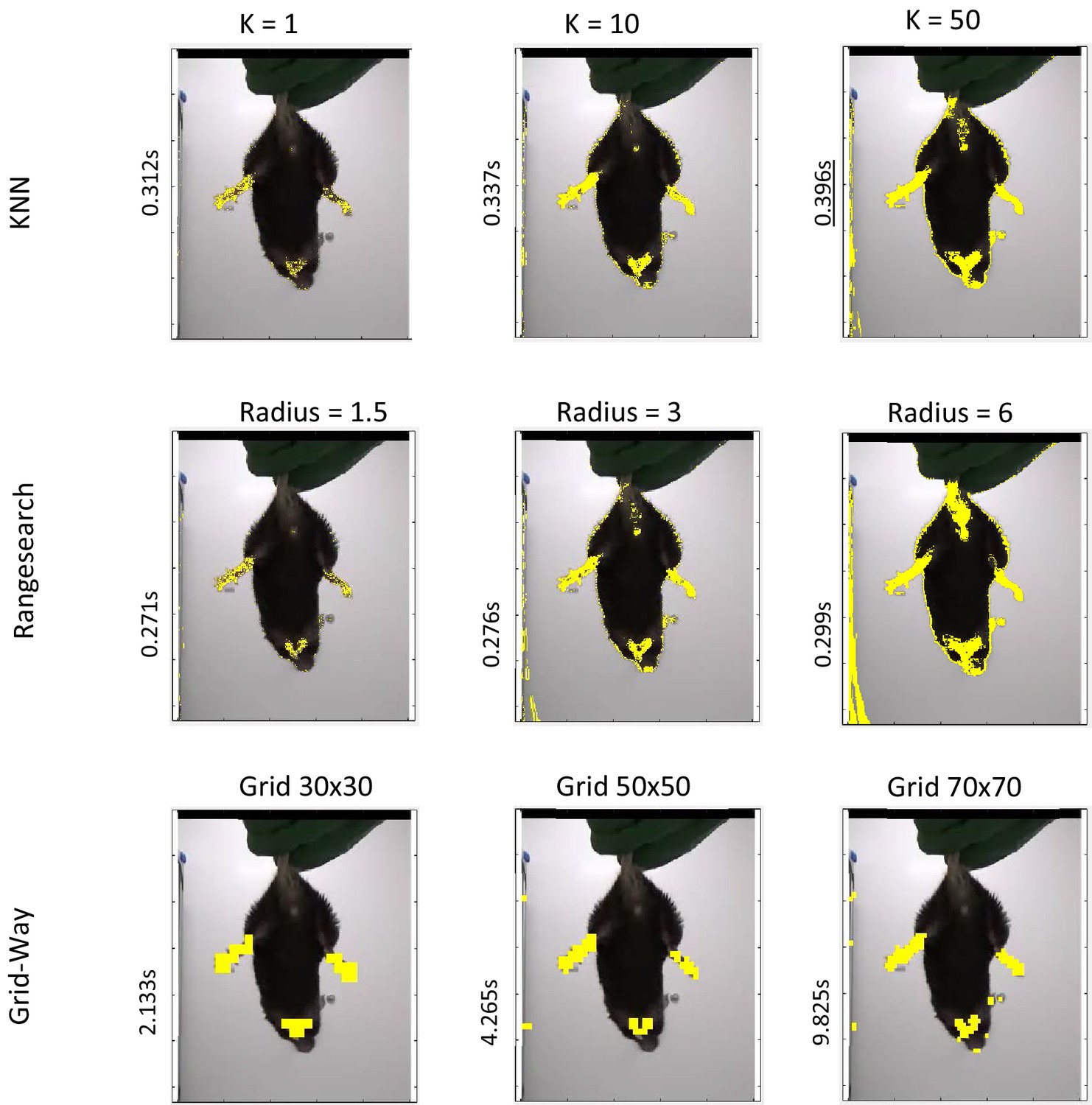
Masks found with KNN, rangesearch, and custrom (grid-way) algorithm.
The Grid-Way produces cleaner masks (eliminating noisy pixels) with sparser identified regions for more efficient subsequent automatic identification of body parts. Masks found for hind paws with three methods. Text on top of each mask shows the respective parameter value used to find the mask and text on the side indicates time taken in seconds to find the mask. Computational time is the largest for the Grid-Way method, but masks are cleaner and easier to operate for heuristic algorithms.
Figure 15—figure supplement 2
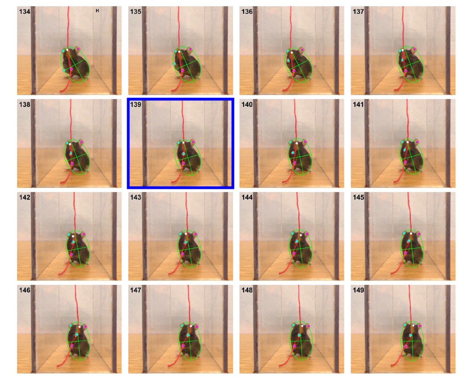
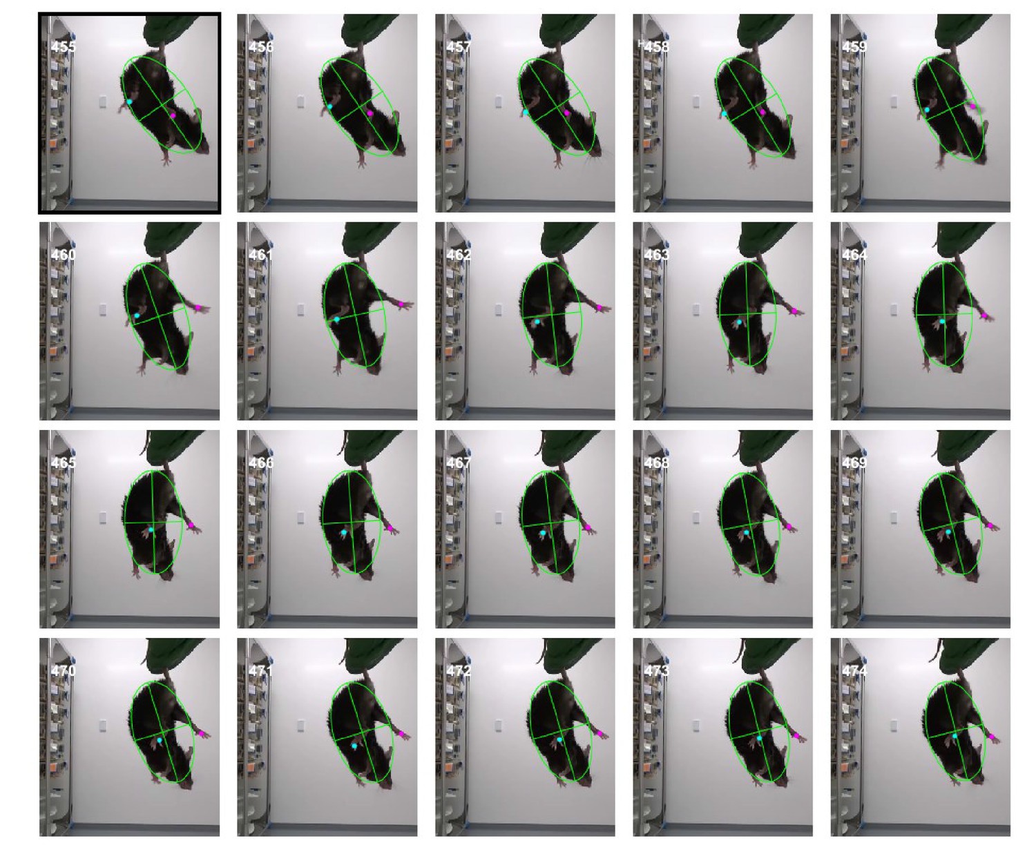
Robustness of image segmentation shown in a video with different camera angle with a mouse on a table with brown base.
Identification of body, ears, nose, and hands was done with 100, 100, 100, and 95 percent accuracy in the 40 frames analyzed for testing image segmentation and tracking algorithms.
Videos
Video 1
Video of the representative.
Black mouse pulling string overlayed with tracked body, ears, nose, and hands also showing frame number and time of frames. Temporal progression of the measured parameters, body length, body angle, head roll angle, head yaw, the X and Y positions of hands from the lower left corner (origin) in the original frames.
Video 2
Same as Video 1 but for White mouse.
Tables
Table 1
Accuracy of algorithms.
Percentage of frames in which a body part was detected automatically. N indicates the number of frames of the string-pulling epoch that was analyzed. (N/A indicates not applicable and values were not used for calculating the overall accuracy. For these situations, either color of a body part was not separable in masks or due to limitation of the camera, hands were blurry in most of the frames).
| Mouse/Body Part | Body | Ears | Nose | Hands |
|---|---|---|---|---|
| Black Mouse 1 (N = 477 of 630) | 100 | 100 | 98.32 | 98.74 |
| Black Mouse 2 (N = 132 of 245) | 100 | 100 | 96.12 | 87.12 |
| Black Mouse 3 (N = 351 of 1435) | 100 | 97.14 | 92.88 | 81.48 |
| Black Mouse 4 (N = 191 of 629) | 100 | 97.38 | 100 | 89.53 |
| Black Mouse 5 (N = 171 of 808) | 100 | 100 | 98.83 | 93.57 |
| Simulated Black Mouse (N = 300 of 477) | 100 | 100 | 100 | 99.67 |
| Mean (Black Mice) | 100 | 99.08 | 97.17 | 91.70 |
| White Mouse 1 (N = 275 of 990) | 100 | 96.36 | 82.91 | 94.91 |
| White Mouse 2 (N = 300 of 594) | 99.67 | 99 | 100 | 91 |
| White Mouse 3 (N = 251 of 453) | 100 | 94.02 | N/A | 60.16 (N/A) |
| White Mouse 4 (N = 166 of 421) | 99.40 | 90.96 | N/A | 30.12 (N/A) |
| White Mouse 5 (N = 216 of 930) | 100 | N/A | N/A | 0 (N/A) |
| Mean (White Mice) | 99.80 | 95.10 | 91.45 | 92.95 |
Additional files
Download links
A two-part list of links to download the article, or parts of the article, in various formats.
Downloads (link to download the article as PDF)
Open citations (links to open the citations from this article in various online reference manager services)
Cite this article (links to download the citations from this article in formats compatible with various reference manager tools)
A Matlab-based toolbox for characterizing behavior of rodents engaged in string-pulling
eLife 9:e54540.
https://doi.org/10.7554/eLife.54540


