Research Article

Bayesian inference for biophysical neuron models enables stimulus optimization for retinal neuroprosthetics

Institute for Ophthalmic Research, University of Tübingen, Germany
Naturwissenschaftliches und Medizinisches Institut an der Universität Tübingen, Germany
Center for Integrative Neuroscience, University of Tübingen, Germany
Bernstein Center for Computational Neuroscience, University of Tübingen, Germany
Department of Neuroscience, University of Pennsylvania, United States
Institute for Bioinformatics and Medical Informatics, University of Tübingen, Germany

Oct 27, 2020

https://doi.org/10.7554/eLife.54997

Open access
Copyright information

Figures
Tables
Additional files

10 figures, 7 tables and 1 additional file

Figures

Figure 1

Download asset Open asset

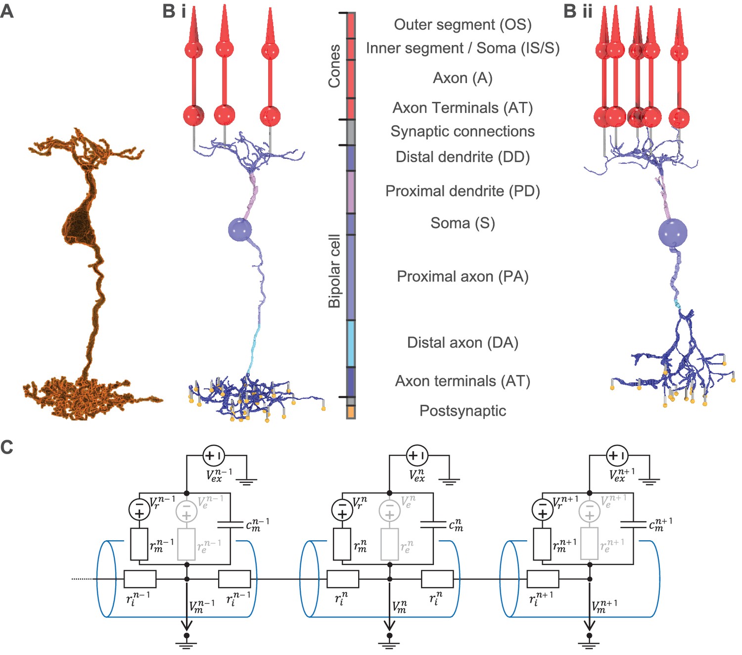
From serial block-face electron microscopy (EM) data of retinal BCs to multicompartment models.

(A) Raw morphology extracted from EM data of an ON-BC of type 5o. (Bi) Processed morphology connected to three presynaptic cones (red) and several postsynaptic dummy compartments that are generated to create the synapses in the model (yellow). The cone and BC morphologies are divided into color-coded regions with a legend shown on the right. (**Bii**) Same as (Bi) but for an OFF-BC of type 3. (C) Three cylindrical compartments of a multicompartment model. Every compartment (blue) n consists of a membrane capacitance $c_{m}^{n}$ , a membrane resistance $r_{m}^{n}$ , a leak conductance voltage source $V_{r}^{n}$ , an extracellular voltage source $V_{e x}^{n}$ and at least one axial resistor $r_{i}^{n}$ that is connected to a neighboring compartment. $V_{e x}^{n}$ is only used to simulate electrical stimulation and is otherwise replaced by a shortcut. Compartments may have one or more further voltage- or ligand-dependent resistances $r_{e}^{n}$ with respective voltage sources $r_{e}^{n}$ to simulate ion channels (indicated in gray).

Figure 2

Download asset Open asset

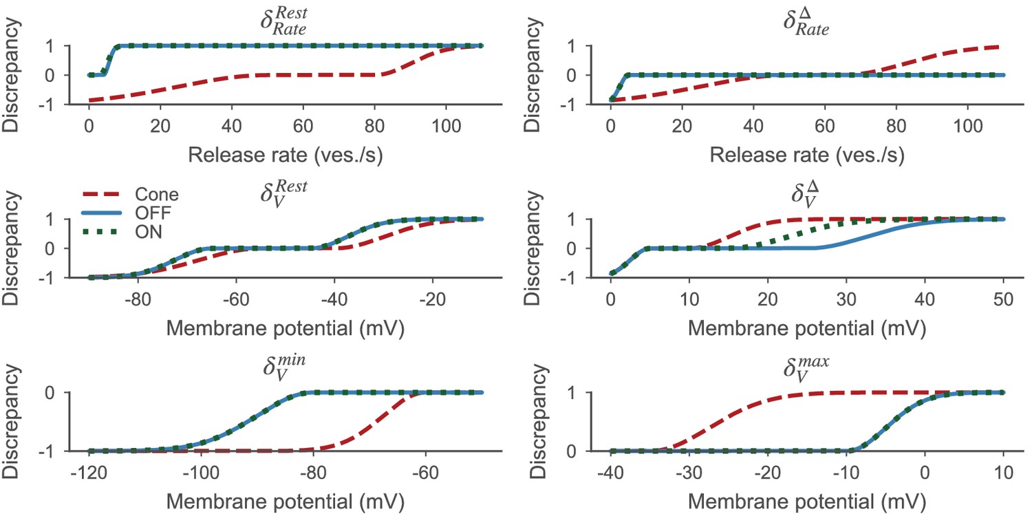
Discrepancy measures based on Equation 13 for the cone (red dashed line), the OFF- (blue solid line) and ON-BC (green dotted line).

The parameters defining the discrepancy measures are listed in Table 3. All discrepancy measures are between zero and one per definition.

Figure 3

Download asset Open asset

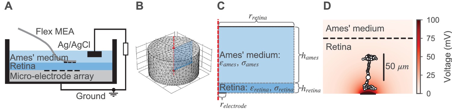
Model for the external electrical stimulation of the retina.

(A) Schematic figure of the experimental setup for subretinal stimulation of ex vivo retina combined with epiretinal recording of retinal ganglion cells. Schematic modified from Corna et al., 2018. (**B,C**) Model for simulating the electrical field potential in the retina in 3D and 2D, respectively. The retina (darker blue) and the electrolyte above (lighter blue) are modeled as cylinders. The shown 3D model is radially symmetric with respect to the central axis (red dashed line). Therefore, the 3D and 2D implementations are equivalent, except that the computational costs for the 2D model are much lower. The 2D implementation is annotated with parameters that were either taken from the literature or inferred from experimental data. (D) Electrical field potential in the retina for a constant stimulation current of 0.5 µA for a single stimulation electrode with a diameter of 30 µm. Additionally, the compartments (black circles with white filling) of the ON-BC model are shown. The stimulation is subretinal meaning that the dendrites are facing the electrode (horizontal black line on bottom).

Figure 4

Download asset Open asset

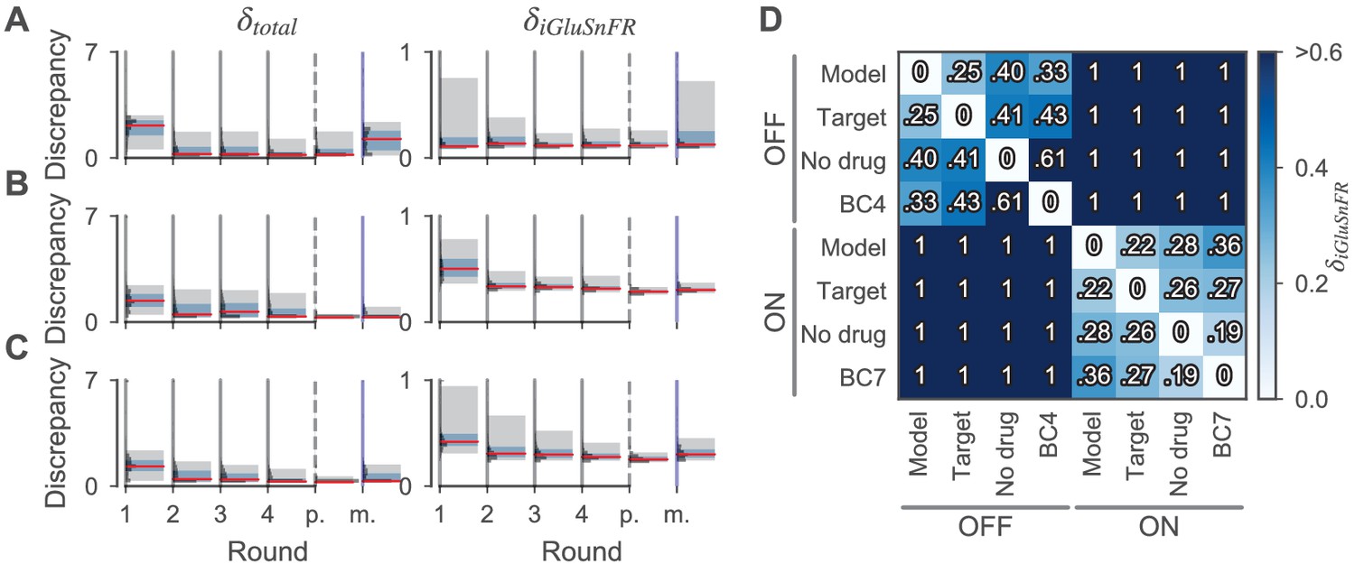
Discrepancies of samples from the cone and the BC models during and after parameter estimation.

(**A, B, C**) Sampled discrepancies for the cone (A), the OFF- (B), and ON-BC (C) respectively. For every model, the total discrepancy $δ_{tot}$ (left) and the discrepancy between the simulated and target iGluSnFR trace $δ_{iGluSnFR}$ (right) are shown. For every model, four optimization rounds with 2000 samples each were drawn (indicated by gray vertical lines). After the last round (indicated by dashed vertical lines, ‘p.’), 200 more samples were drawn from the posteriors. For the BCs, the number of compartments was increased in this last step to 139 and 152 for the OFF- and ON-BC, respectively. Additionally, 200 samples were drawn from assuming independent posterior marginals for comparison (indicated by blue vertical lines, ‘m.’). For every round, the discrepancy distribution (horizontal histograms), the median discrepancies (red vertical lines), the 25th to 75th percentile (blue shaded area) and the 5th to 95th percentile (gray-shaded area) are shown. (D) Discrepancies between different iGluSnFR traces of BCs to demonstrate the high precision of the model fit. The pairwise discrepancy computed with equation Equation 12 between eight iGluSnFR traces is depicted in a heat map. The column and row labels indicate which $𝝂_{t}$ and $𝝂_{m}$ were used in equation Equation 12 respectively. The traces consists of the optimized BC models (‘Model’), the targets used during optimization (‘Target’), experimental data from the same cell type without the application of any drug (‘No drug’) and experimental data from another retinal CBC type with the application of strychnine (‘BC4’ and ‘BC7’). Note that strychnine was also applied to record the targets.

Figure 4—source data 1 Sample discrepancies of all samples shown in (A-C).: https://cdn.elifesciences.org/articles/54997/elife-54997-fig4-data1-v2.zip
Download elife-54997-fig4-data1-v2.zip
Figure 4—source data 2 Discrepancies shown in (D), and the respective (mean) iGluSnFR traces.: https://cdn.elifesciences.org/articles/54997/elife-54997-fig4-data2-v2.zip
Download elife-54997-fig4-data2-v2.zip

Figure 5 with 2 supplements

Download asset Open asset

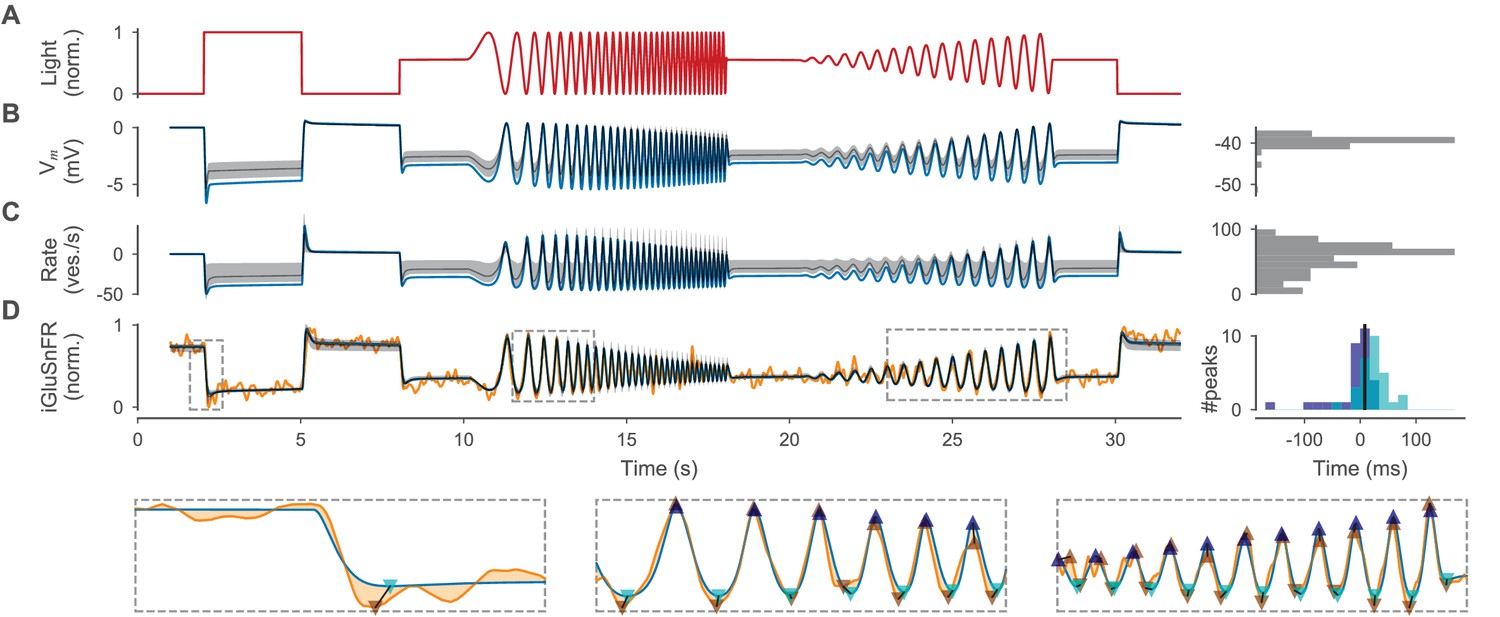
Optimized cone model.

(A) Normalized light stimulus. (B) Somatic membrane potential relative to the resting potential for the best parameters (blue line) and for 200 samples from the posterior shown as the median (gray dashed line) and 10th to 90th percentile (gray shaded area). A histogram over all resting potentials is shown on the right. (C) Release rate relative to the resting rate. Otherwise as in (B). (D) Simulated iGluSnFR trace (as in (B)) compared to target trace (orange). Three regions (indicated by gray dashed boxes) are shown in more detail below without samples from the posterior. Estimates of positive and negative peaks are highlighted (up- and downward facing triangles respectively) in the target (brown) and in the simulated trace (blue and cyan respectively). Pairwise time differences between target and simulated peaks (indicated by triangle pairs connected by a black line) are shown as histograms for positive (blue) and negative (cyan) peaks on the right. The median over all peak time differences is shown as a black vertical line.

Figure 5—source data 1 iGluSnFR traces used for constraining the cone and BC models.: https://cdn.elifesciences.org/articles/54997/elife-54997-fig5-data1-v2.zip
Download elife-54997-fig5-data1-v2.zip
Figure 5—source data 2 Stimulus, target, and cell responses, including responses with removed ion channels.: https://cdn.elifesciences.org/articles/54997/elife-54997-fig5-data2-v2.zip
Download elife-54997-fig5-data2-v2.zip

Figure 5—figure supplement 1

Download asset Open asset

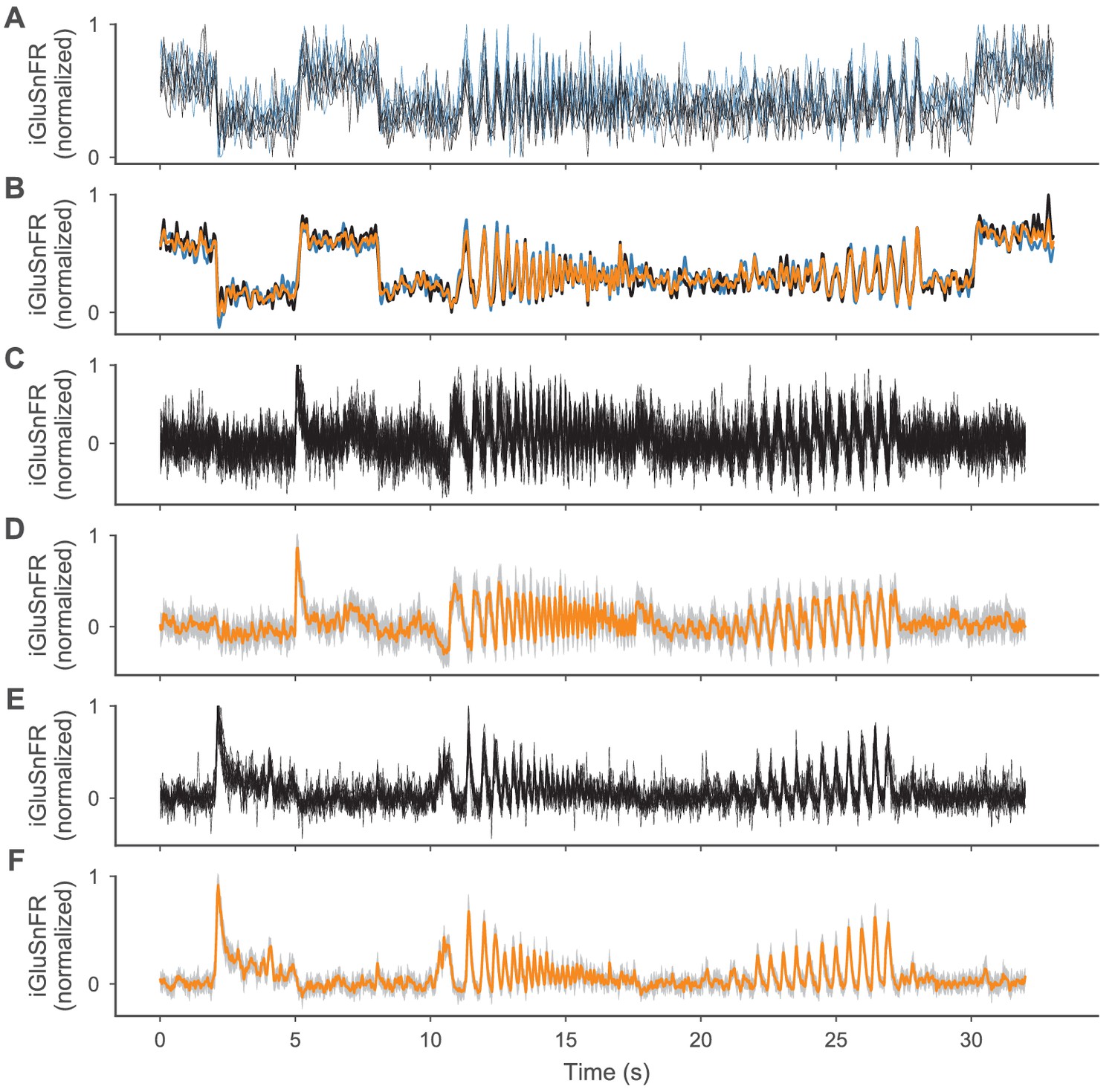
iGluSnFR traces used for constraining the cone and BC models.

iGluSnFR traces used for constraining the cone and BC models. (**A,C,E**) All single ROI traces used for the cone, OFF- and ON-BC, respectively. For the cone, the traces are shown in different colors for the two recorded axon terminals. (B) Aligned mean traces of both cone axon terminals (same colors as in (A)), and the mean of both means (orange), which was used as the target during parameter inference. (**D,F**) Mean traces (orange) plus-minus one standard deviation (gray-shaded area) across all single ROI traces for the OFF- and ON-BC, respectively.

Figure 5—figure supplement 2

Download asset Open asset

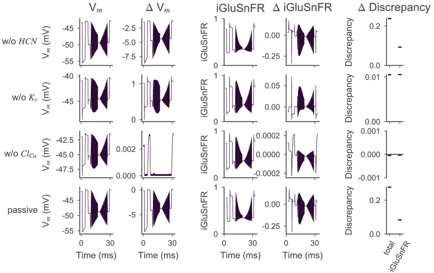
Effect of active ion conductances on the optimized cone model.

Voltage and iGluSnFR traces for the optimized cone model with different ion channels removed. In every row, a different (set of) ion channels has been removed from the model by setting the respective conductances to zero. The simulated somatic membrane voltages (first column) and iGluSnFR traces (third column) and the differences with respect to the simulation with all ion channels (second and fourth column, respectively) are shown. The fifth column shows how removing the ion channel changed the total discrepancy $δ_{tot}$ and distance to the experimental target $δ_{iGluSnFR}$ . The row titles refer to the channel that has been removed, for example in the first row, the HCN channel has been removed. In the last row (passive), all but the calcium channels in the axon terminals were removed.

Figure 6 with 6 supplements

Download asset Open asset

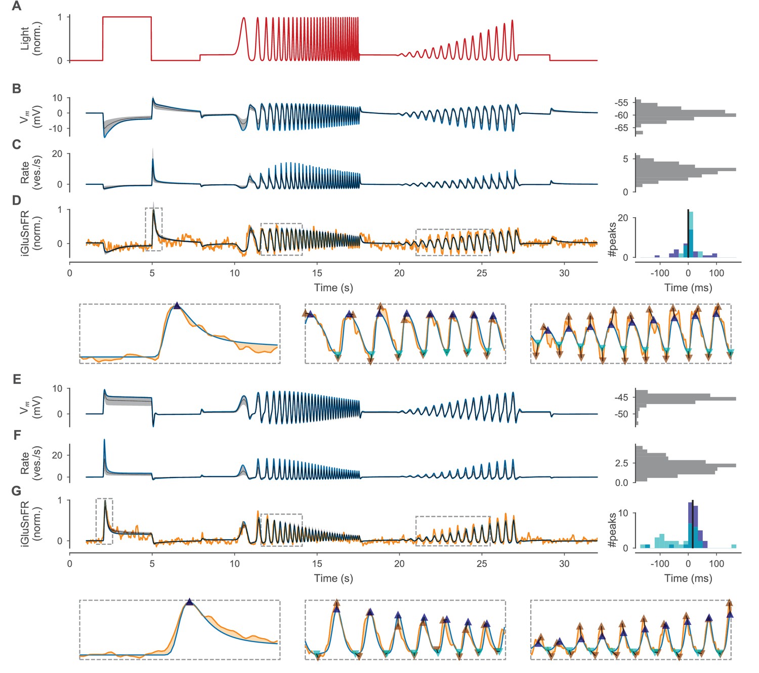
Optimized BC models.

(A) Normalized light stimulus. Responses of the OFF- and ON-BC are shown in (**B–D**) and (**E–G**), respectively. (**B, E**) Somatic membrane potential relative to the resting potential for the best parameters (blue line) and for 200 samples from the posterior shown as the median (gray dashed line) and 10th to 90th percentile (gray-shaded area). A histogram over all resting potentials is shown on the right. (**C, F**) Mean release rate over all synapses relative to the mean resting rate. Otherwise as in (B). (**D, G**) Simulated iGluSnFR trace (as in (B)) compared to respective target trace (orange). Three regions (indicated by gray dashed boxes) are shown in more detail below without samples from the posterior. Estimates of positive and negative peaks are highlighted (up- and downward facing triangles, respectively) in the target (brown) and in the simulated trace (blue and cyan, respectively). Pairwise time differences between target and simulated peaks (indicated by triangle pairs connected by a black line) are shown as histograms for positive (blue) and negative (cyan) peaks on the right. The median over all peak time differences is shown as a black vertical line.

Figure 6—source data 1 Stimulus, target, and cell responses, including responses with removed ion channels.: https://cdn.elifesciences.org/articles/54997/elife-54997-fig6-data1-v2.zip
Download elife-54997-fig6-data1-v2.zip

Figure 6—figure supplement 1

Download asset Open asset

Heatmaps of the OFF-BC.

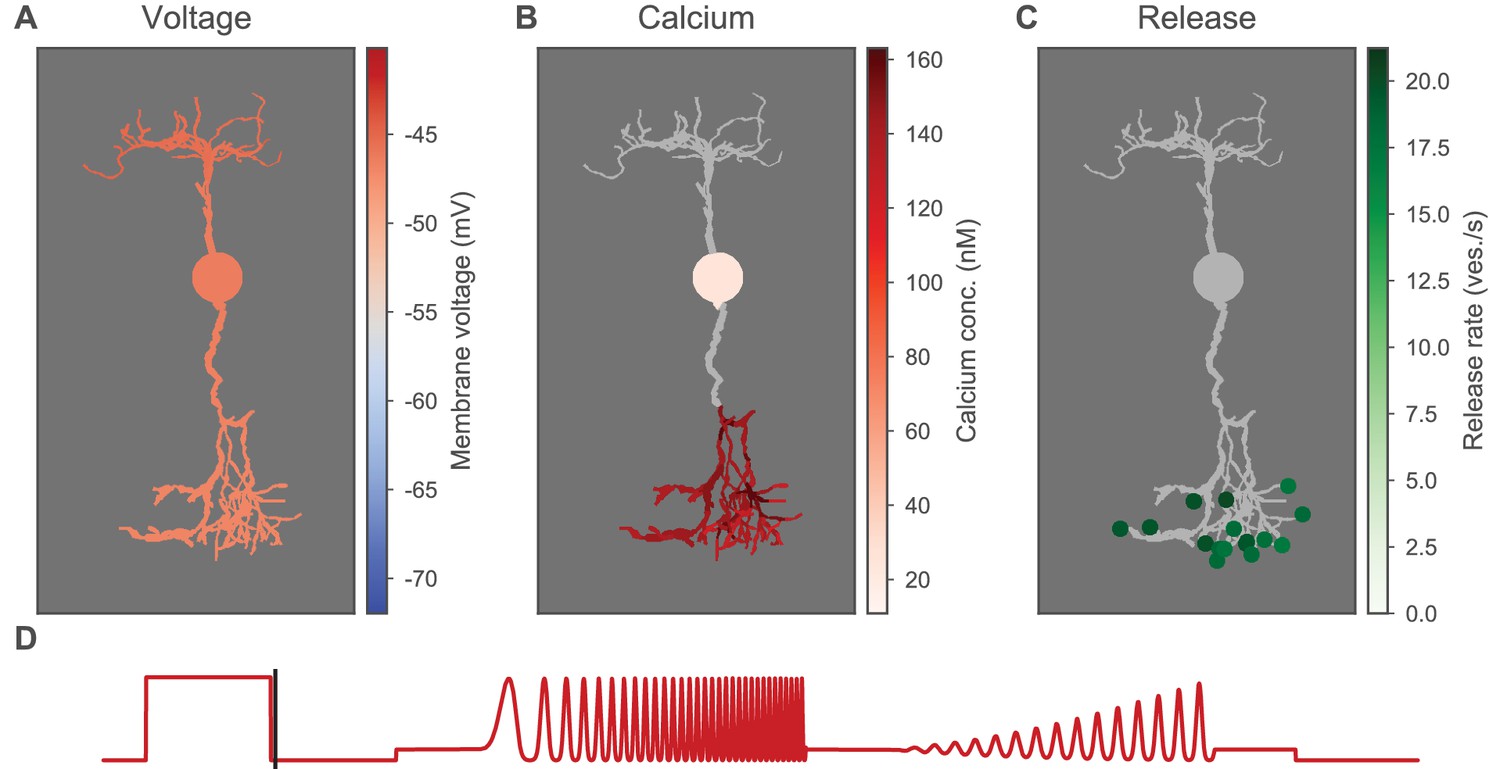
Heatmaps of the OFF-BC in response to the OFF-step of the light stimulus. A video for the full stimulus is available in the supplementary material. (A) Membrane voltage (color-coded) of all compartments mapped on fully detailed morphology. (B) Calcium concentration (color-coded) in BC for all compartments for which calcium is simulated. Other compartments are shown in gray. (C) Release sites with color-coded release rates (green dots). Compartments are shown in gray. (D) Light stimulus. The time for which the heatmaps are shown is indicated by the black vertical line.

Figure 6—figure supplement 2

Download asset Open asset

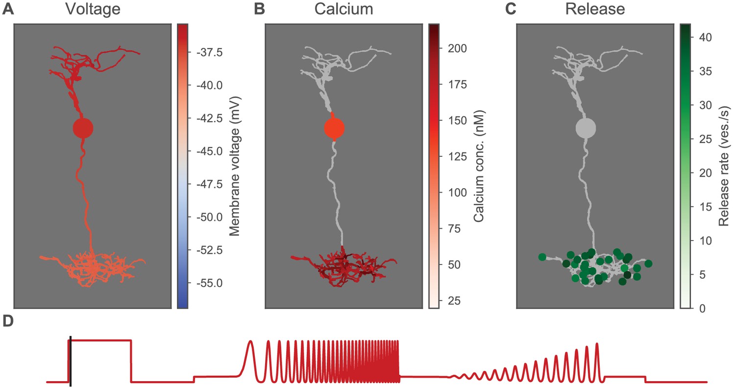
Heatmaps of the ON-BC.

Heatmaps of the ON-BC in response to the ON-step of the light stimulus; otherwise as in Figure 6—figure supplement 1.

Figure 6—figure supplement 3

Download asset Open asset

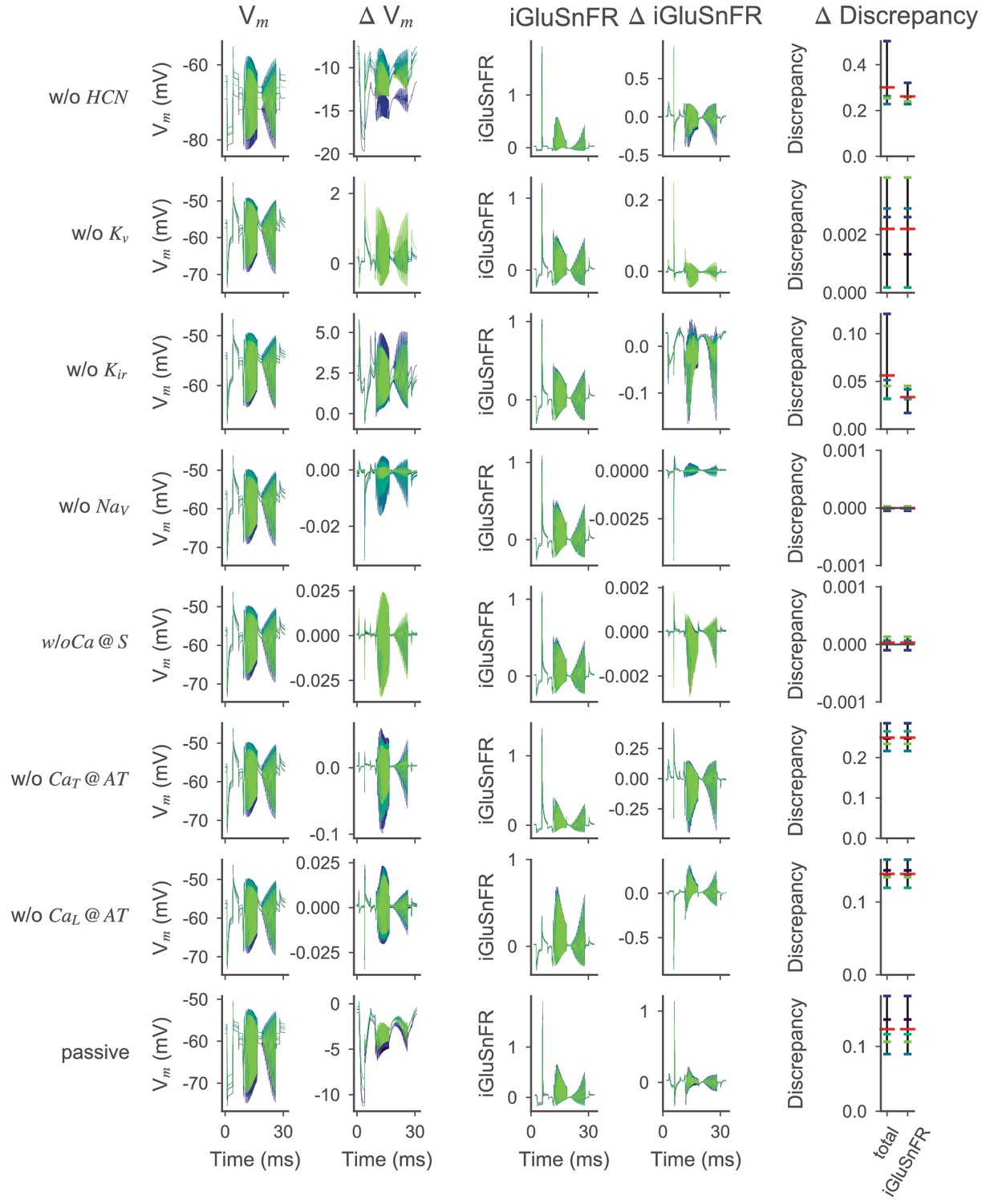
Effect of active ion conductances on the optimized OFF-BC model.

Voltage and iGluSnFR traces for the OFF-BC with different ion channels removed. Models were simulated for the five posterior samples (out of 200) with the lowest total discrepancy $δ_{tot}$ under different conditions. The samples are color-coded across all panels. In every row, a different (set of) ion channels has been removed from the posterior samples by setting the respective conductances to zero. The simulated somatic membrane voltages (first column) and iGluSnFR traces (third column) and the differences with respect to the simulation with all ion channels (second and fourth column, respectively) are shown. The fifth column shows how removing the ion channel changed the total discrepancy $δ_{tot}$ and distance to the experimental target $δ_{iGluSnFR}$ for all samples individually (small vertical lines) and as a mean over all samples (red vertical line). The row titles refer to the channel that has been removed, for example in the first row, the HCN channel has been removed. Ca @ S means, that all somatic calcium channels were removed. In the last row (passive), all but the calcium channels in the axon terminals were removed.

Figure 6—figure supplement 4

Download asset Open asset

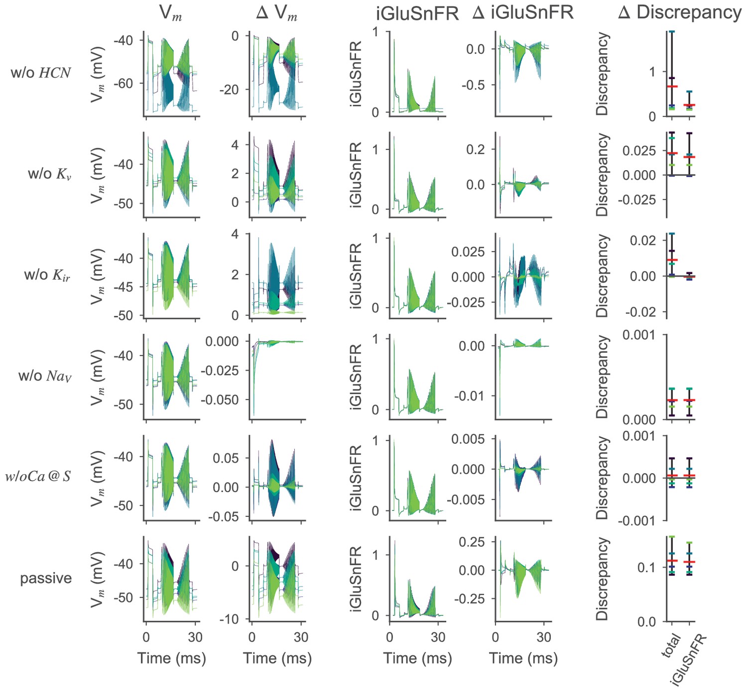
Effect of active ion conductances on the optimized ON-BC model.

Voltage and iGluSnFR traces for the ON-BC with different ion channels removed; otherwise as in Figure 6—figure supplement 3.

Figure 6—video 1

Download asset

posterframe for video — Animated heatmaps of the OFF-BC.

Figure 6—video 2

Download asset

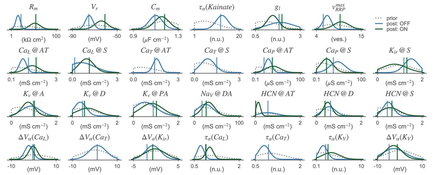
Figure 7 with 2 supplements

Download asset Open asset

Parameter distributions of the BC models.

1D-marginal prior (dashed gray line) and posterior distributions (solid lines) are shown for the OFF- (blue) and ON-BC (green). The parameters of the posterior samples with the lowest total discrepancy are shown as dashed vertical lines in the respective color. $X_{Y} @ Z$ refers to the channel density of channel $X_{Y}$ at location $Z$ . Locations are abbreviated; S: soma, A: axon, D: dendrite and AT: axon terminals (see Figure 1 and main text for details). Note that although these 1D-marginal distributions seem relatively wide in some cases, the full high-dimensional posterior has much more structure than a posterior distribution obtained from assuming independent marginals (see Figure 4). Not all parameter distributions are shown.

Figure 7—source data 1 Prior and posterior parameters for the OFF- and ON-BC.: https://cdn.elifesciences.org/articles/54997/elife-54997-fig7-data1-v2.zip
Download elife-54997-fig7-data1-v2.zip

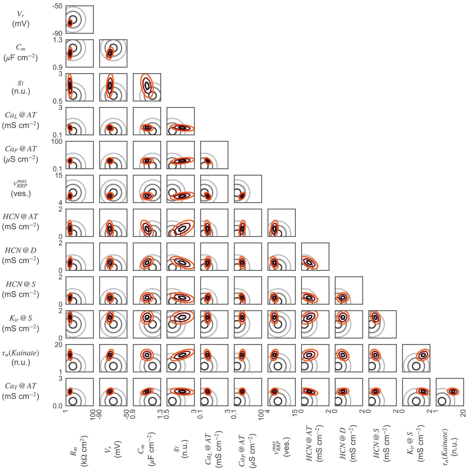
Figure 7—figure supplement 1

Download asset Open asset

2D-marginals for the OFF-BC.

Parameter distributions of the OFF-BC model. 2D-marginal prior (gray) and posterior distributions (red). Distributions are shown as contour lines at 30, 60 and 90% of the maximum of the respective probability density functions. Not all parameter distributions are shown.

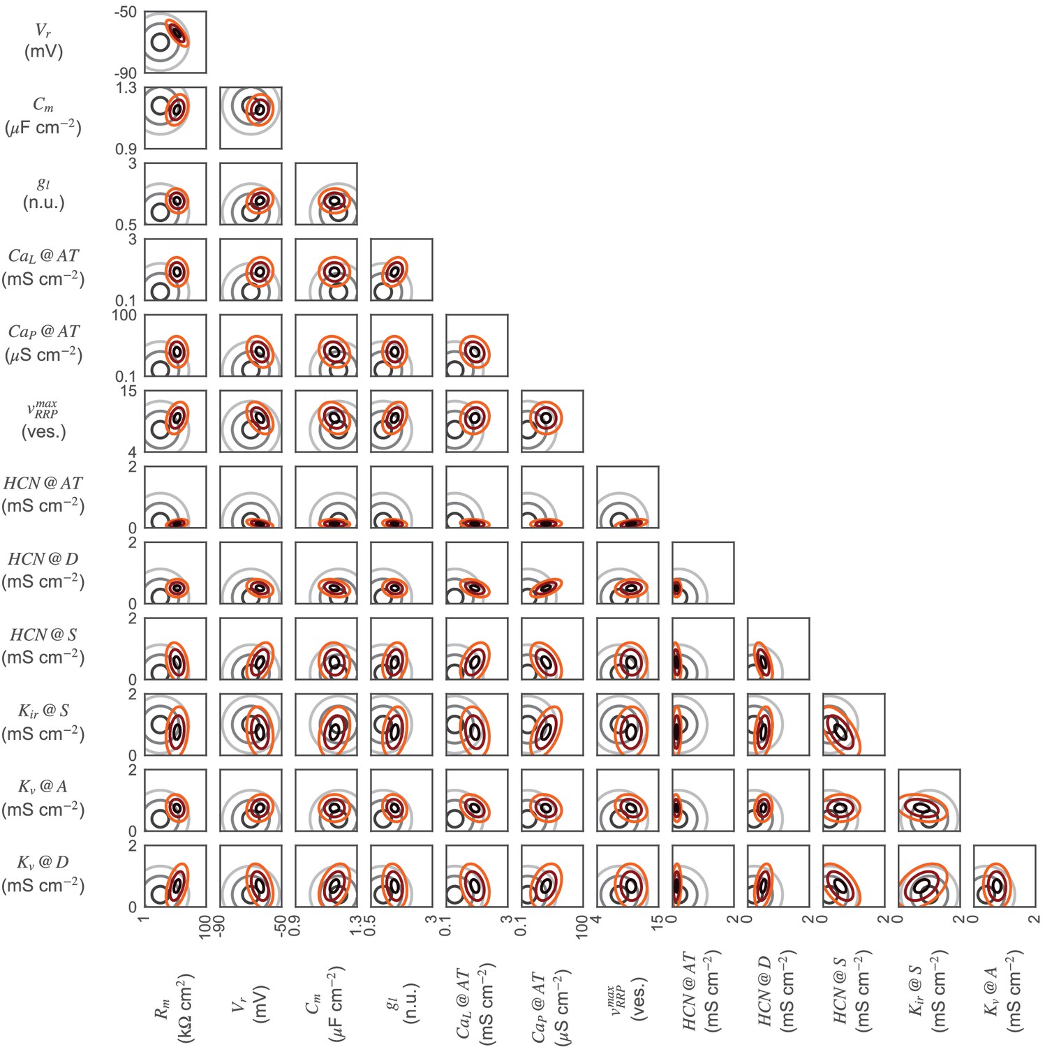
Figure 7—figure supplement 2

Download asset Open asset

2D-marginals for the ON-BC.

Parameter distributions of the ON-BC model. 2D-marginal prior (gray) and posterior distributions (red). Distributions are shown as contour lines at 30, 60, and 90% of the maximum of the respective probability density functions. Not all parameter distributions are shown.

Figure 8

Download asset Open asset

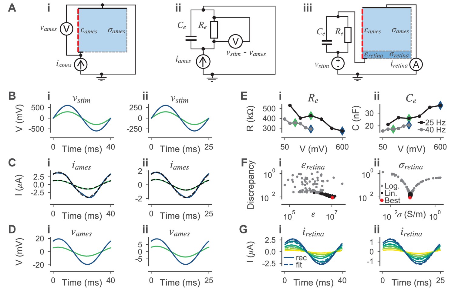
Estimation of the conductivity $σ_{retina}$ and the relative permittivity $ε_{retina}$ of the retina for simulating electrical stimulation.

(A) Electrical circuits used during parameter estimation. (B) Stimulation voltages $v_{stim}$ at 25 (left) and 40 Hz (right). From the six experimentally applied amplitudes, only the amplitudes used for parameter inference are shown. (C) Experimentally measured currents $i_{ames}$ through electrolyte (Ames’ solution) without retinal tissue for the stimulus voltages $v_{stim}$ in (B). The mean traces over all (but the first two) repetitions are shown (black dashed lines). Sine waves were fitted to the mean traces (solid lines) with colors referring to the voltages in (B). (D) Simulated voltages over the electrolyte $v_{ames}$ using the fitted currents in (C) as stimuli applied to the circuit in (Ai). (Aii) Electrical circuit used to model the electrode plus interface. (E) Stimulus frequency and amplitude dependent estimates of $R_{e}$ (i) and $C_{e}$ (ii) based on the electrical circuit shown in (Aii) for 25 (black) and 40 Hz (gray). Note that the values were derived analytically (see main text). The values corresponding to the stimulus voltages shown in (B) are highlighted with respective color. (Aiii) Electrical circuit used to estimate $σ_{retina}$ and $ε_{retina}$ . The respective values for $R_{e}$ and $C_{e}$ are shown in (E) and are dependent on $v_{stim}$ . The current $i_{retina}$ through the model is measured for a given stimulus voltage $v_{stim}$ . (F) Sampled parameters of $ε_{retina}$ and $σ_{retina}$ and the respective sample losses. First, samples were drawn in a wide logarithmic space (gray dots) and then in a narrower linear parameter space. The best sample (lowest discrepancy) is highlighted in red. (G) Simulated currents $i_{retina}$ (solid lines) through the circuit in (Aiii) with optimized parameters (red dot in (F)) and respective experimentally measured currents (broken lines). Here, results for all six stimulus amplitudes are shown for both frequencies.

Figure 8—source data 1 Currents, voltages, and samples from optimization.: https://cdn.elifesciences.org/articles/54997/elife-54997-fig8-data1-v2.zip
Download elife-54997-fig8-data1-v2.zip

Figure 9

Download asset Open asset

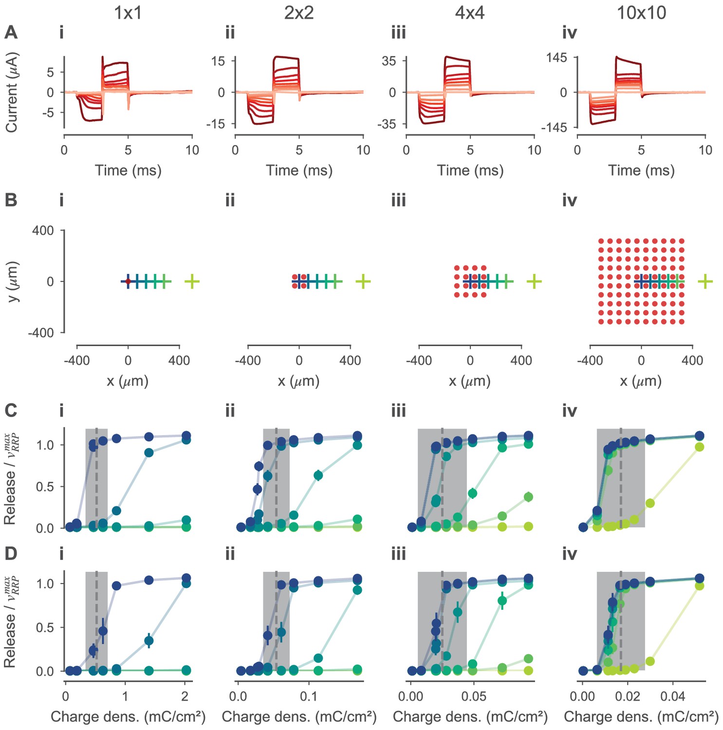
Threshold of electrical stimulation for experimentally measured RGCs and simulated BCs of photoreceptor degenerated mouse retina.

(A) Stimulation currents measured experimentally and used as stimuli in the simulations. (B) xy-positions of BCs (crosses) and electrodes (red dots) for 1×1, 2×2, 4×4, 10×10 stimulation electrodes, respectively. Every electrode is modeled as a disc with a 30 µm diameter. Except for the electrode configuration, the models were as in Figure 8. (**C, D**) Mean synaptic glutamate release relative to the size of the readily releasable pool $v_{RRP}^{max}$ of simulated OFF- and ON-BCs, respectively. Values can be greater than 1, because the pool is replenished during simulation. Errorbars indicate the standard deviation between simulations of BCs with different parametrizations; for both BCs, the five best posterior samples were simulated. Glutamate release is shown for different charge densities (x-axis) and cell positions (colors correspond to xy-positions in (A); for example the darkest blue corresponds to the central BC). Experimentally measured RGC thresholds (gray dashed lines) plus-minus one standard deviation (gray-shaded ares) are shown in the same plots.

Figure 9—source data 1 Current traces and vesicle release for all simulations.: https://cdn.elifesciences.org/articles/54997/elife-54997-fig9-data1-v2.zip
Download elife-54997-fig9-data1-v2.zip

Figure 10 with 1 supplement

Download asset Open asset

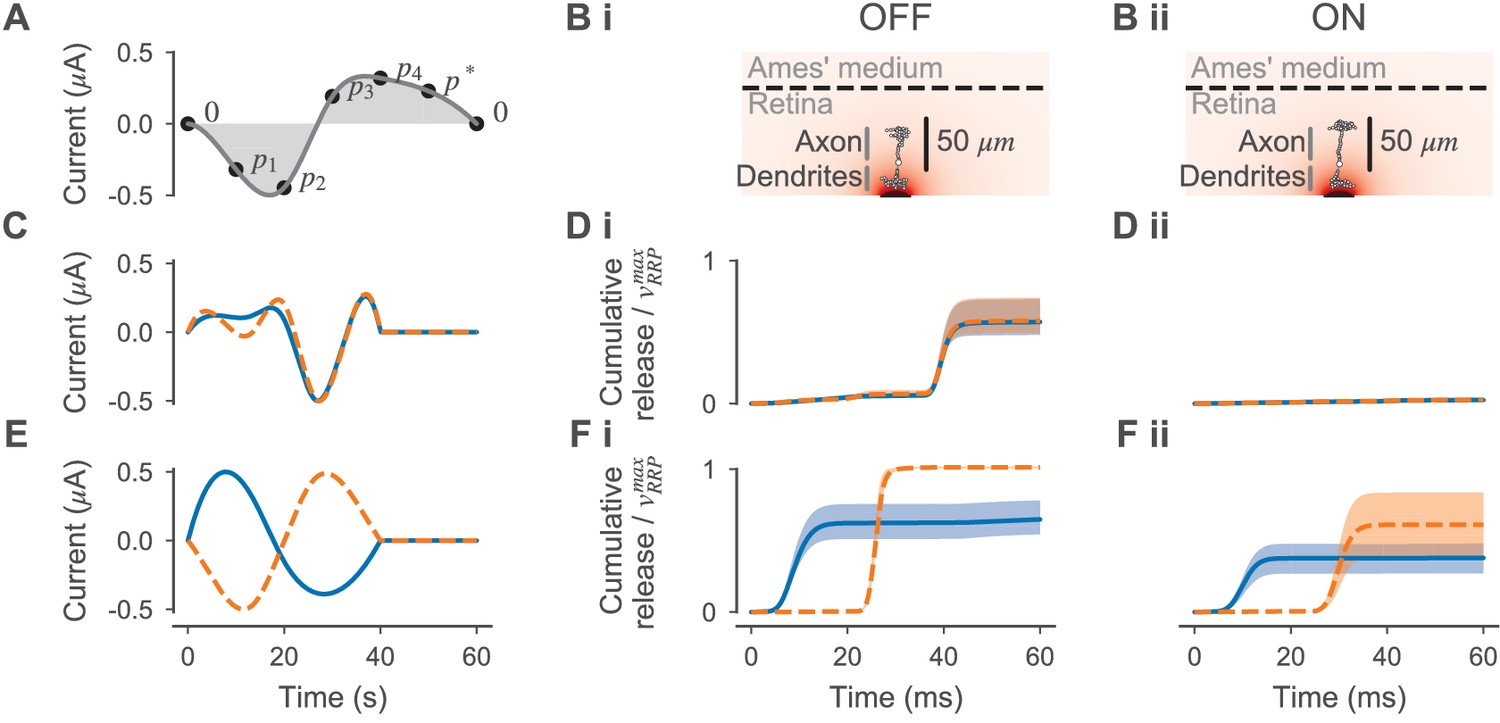
Electrical currents optimized for selective ON- and OFF-BC stimulation.

(A) Illustration of the stimulus parametrization. A stimulation current was computed by fitting a cubic spline through points defined by $p_{1} \dots p_{4}$ and $p^{*}$ (black dots) that were placed equidistantly in time. $p_{1} \dots p_{4}$ were free parameters and $p^{*}$ was chosen such that the stimulus was charge neutral, that is the integral over the current (gray-shaded area) was zero. Currents were normalized such that the maximum amplitude was always 0.5 µA. (B) Illustration of the electrical stimulation of an OFF- (i) and ON-BC (ii) multicompartment model. (**C, E**) Stimuli optimized for selective OFF- and ON-BC stimulation, respectively. The two best stimuli observed during optimization are shown. (**D, F**) Cumulative vesicle release (as a mean over all synapses) relative to the size of the readily releasable pool $v_{RRP}^{max}$ in response to the electrical stimuli shown in (C) and (E), respectively. Stimuli and responses are shown in matching colors. Release is shown for the five best posterior cell parametrizations for the OFF- (i) and ON-BC (ii) as a mean (line) plus-minus one standard deviation (shaded area).

Figure 10—source data 1 Optimized stimuli and BC responses, including responses with removed ion channels.: https://cdn.elifesciences.org/articles/54997/elife-54997-fig10-data1-v2.zip
Download elife-54997-fig10-data1-v2.zip

Figure 10—figure supplement 1

Download asset Open asset

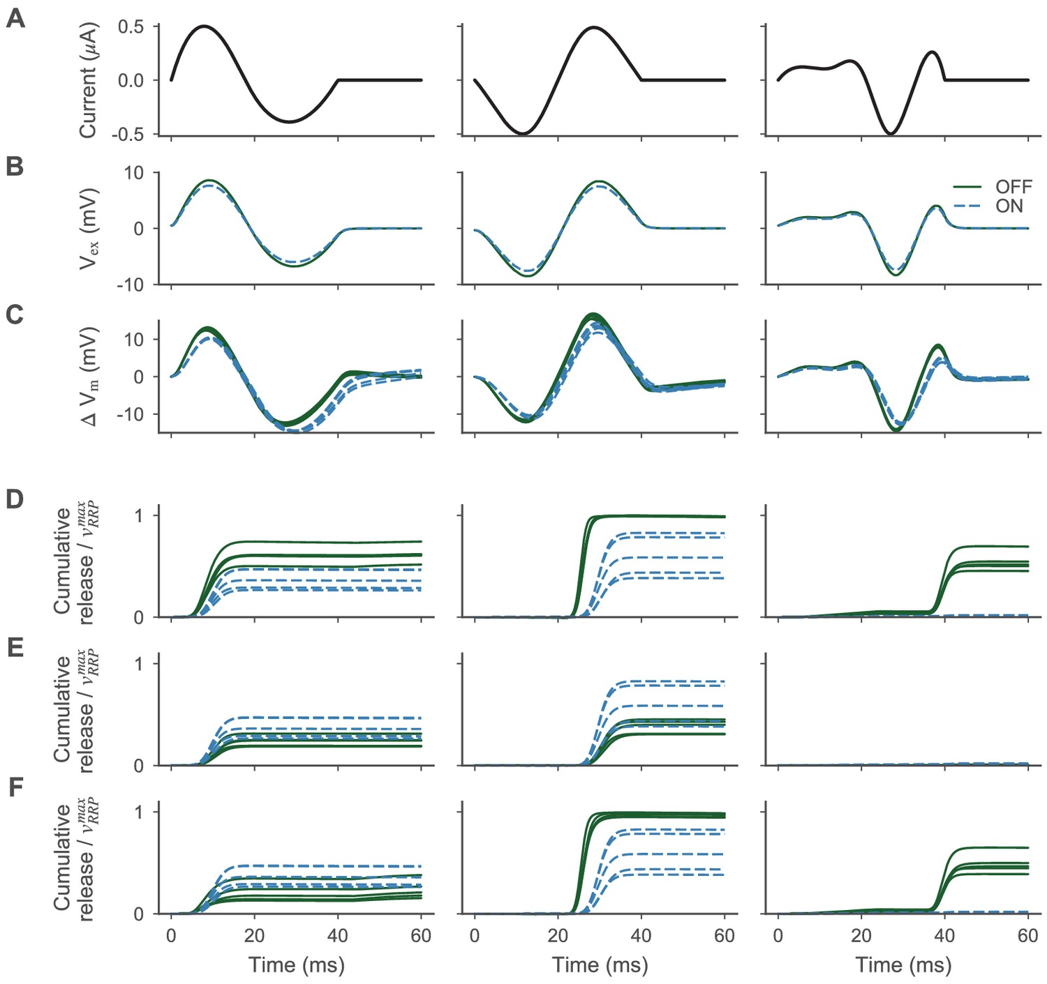
Electrical stimulation with optimized stimuli and removed ion channels.

Electrical stimulation with optimized stimuli and selectively removed ion channels. (A) Stimulation currents optimized to selectively stimulate the ON- (left and middle) and OFF-BC (right). (B) Evoked extracellular voltage at the presynaptic BC compartments (as a mean over all synapses) for the OFF- (blue) and ON-BC (green), respectively. (C) Change of the membrane voltage during stimulation at the presynaptic BC compartments for the five best posterior BC parametrizations. Otherwise as in (B). (D) Cumulative vesicle release (as a mean over all synapses) relative to the size of the readily releasable pool $v_{RRP}^{max}$ for the same BC parametrizations. (E) As in (D), but the ${Ca}_{T}$ channels at the axon terminals of the OFF-BC were removed. (F) As in (D), but the ${Ca}_{L}$ channels at the axon terminals of the OFF-BC were removed.

Tables

Key resources table

Reagent type (species) or resource	Designation	Source or reference	Identifiers	Additional information
Genetic reagent (mouse)	B6;129S6-Chat^{tm2(cre)LowlJ}	Jackson laboratory JAX 006410	RRID:IMSR_JAX:006410
Genetic reagent (mouse)	Gt(ROSA)26Sor ^{tm9(CAG-tdTomato)Hze}	Jackson laboratory JAX 007905	RRID:IMSR_JAX:007905
Strain (mouse, female)	B6.CXB1-Pde6b^rd10	Jackson laboratory JAX 004297	RRID:IMSR_JAX:004297
Strain (Adeno-associated virus)	AAV2.7m8.hSyn.iGluSnFR	Virus facility, Institute de la Vision, Paris
Software, algorithm	NeuronC	https://retina.anatomy.upenn. edu/rob/neuronc.html	RRID:SCR_014148	Version 6.3.14
Software, algorithm	SNPE	https://github.com/mackelab/delfi		See Inference algorithm
Software, algorithm	COMSOL Multiphysics	COMSOL Multiphysics	RRID:SCR_014767

Table 1

Ion channels of biophysical models.

Channel	Cone	OFF-BC (type 3a)	ON-BC (type 5)	Cone references	BC references
${C a}_{L}$	AT	S, AT	S, AT	Morgans et al., 2005; Mansergh et al., 2005	Van Hook et al., 2019
${C a}_{T}$		S, AT			Van Hook et al., 2019
${C a}_{P}$	AT	S, AT	S, AT	Morgans et al., 1998	Morgans et al., 1998
${H C N}_{1}$	All		D, S, AT	Knop et al., 2008; Van Hook et al., 2019	Knop et al., 2008; Hellmer et al., 2016
${H C N}_{4}$		D, S, AT			Hellmer et al., 2016; Knop et al., 2008
$K_{V}$	IS/S	DD, PA, DA	DD, PA, DA	Knop et al., 2008; Van Hook et al., 2019	Ma et al., 2005
$K_{i r}$		S	S		Cui and Pan, 2008; Knop et al., 2008
${C l}_{C a}$	AT			Yang et al., 2008; Caputo et al., 2015
${N a}_{V}$		DA	DA		Hellmer et al., 2016

Regions of ion channels and the respective abbreviations as in Figure 1.

D refers to the combination of DD and PD. All refers to the combination of IS/S, A, and AT.
If multiple regions are stated for a neuron, the ion channel density differs between them.

Table 2

Ion channel implementation details and optimized channel parameters.

Channel	NeuronC	Type	States	Parameters	Channel remarks and references
Kainate rec.	AMPA1	MS	7	$S T C$ , $τ_{γ}$	Based on Jonas et al., 1993.
mGluR6	mGluR			$S T C$	See NeuronC documenation.
${C a}_{L}$	CA0	HH	(4)	$Δ V_{α}$ , $τ_{α}$	Based on Karschin and Lipton, 1989.
${C a}_{T}$	CA7	MS	12	$Δ V_{α}$ , $τ_{α}$	Modification of Lee et al., 2003.
${C a}_{P}$				${C a}_{P K}$	See NeuronC documenation.
${H C N}_{1 / 2 / 4}$	K4	MS	10		Based on Altomare et al., 2001.
$K_{V}$	K0	HH	(5)	$Δ V_{α}$ , $τ_{α}$	Based on Hodgkin and Huxley, 1952.
$K_{i r}$	K5	MS	3	$Δ V_{α}$	Modification of Dong and Werblin, 1995.
${C l}_{C a}$	CLCA1	MS	12		Modification of Hirschberg et al., 1998.
${N a}_{V}$	NA5	MS	9	$Δ V_{α}$ , $Δ V_{γ}$ , $τ_{all}$	Based on Clancy and Kass, 2004.

Table 3

Parameters of discrepancy measures.

$δ_{∙}^{∙}$	Cone				BC (3a \| 5o)				References
	$p_{l}$	$t_{l}$	$t_{u}$	$p_{u}$	$p_{l}$	$t_{l}$	$t_{u}$	$p_{u}$
$δ_{Rate}^{Rest}$	0	50	80	100	0	0	3 \| 4	7	Choi et al., 2005; Sheng et al., 2007; Berntson and Taylor, 2003; Singer and Diamond, 2006
$δ_{V}^{Rest}$	−80	−55	−40	−20	−80	−65	−45	−30	Cangiano et al., 2012; Ichinose et al., 2014; Ichinose and Hellmer, 2016; Ma et al., 2005
$δ_{Rate}^{Δ}$	0	50	65	100	0	5	∞	∞
$δ_{V}^{Δ}$	0	5	10	20	0	5	15 \| 25	40	Ichinose et al., 2014; Ichinose and Hellmer, 2016
$δ_{V}^{m i n}$	−75	60	∞	∞	−100	−80	∞	∞	Cangiano et al., 2012; Ma et al., 2005; Saszik and DeVries, 2012
$δ_{V}^{m a x}$	$- \infty$	$- \infty$	−35	−20	$- \infty$	$- \infty$	−10	0	Cangiano et al., 2012; Ma et al., 2005; Saszik and DeVries, 2012

Appendix 1—table 1

Cone model parameter priors.

Parameter	Unit	a_i	µ_i	b_i	References: direct and additional
$C_{m}$	$μ F {c m}^{- 2}$	0.9	1	1.3	Oltedal et al., 2009
$R_{m}$	$k Ω {c m}^{2}$	1	5	100	Oltedal et al., 2009
$V_{r}$	$mV$	-90	-70	-50
${C a}_{L}$	$m S {c m}^{- 2}$	0.1	2	10	Morgans et al., 2005; Mansergh et al., 2005; Cui et al., 2012
$K_{V}$	$m S {c m}^{- 2}$	0	0.1	3	Van Hook et al., 2019
$H C N @ S$	$m S {c m}^{- 2}$	0	3	10	Knop et al., 2008; Hellmer et al., 2016; Van Hook et al., 2019
$H C N @ A$	$m S {c m}^{- 2}$	0	1	10	Knop et al., 2008; Hellmer et al., 2016; Van Hook et al., 2019
$H C N @ A T$	$m S {c m}^{- 2}$	0	0.1	10	Knop et al., 2008; Hellmer et al., 2016; Van Hook et al., 2019
${C l}_{C a}$	$m S {c m}^{- 2}$	0	0.1	10	Yang et al., 2008; Caputo et al., 2015
${C a}_{P}$	$μ S {c m}^{- 2}$	0.1	10	100	Morgans et al., 1998
$τ_{α} ({C a}_{L})$		0.75	1	1.5
$τ_{α} (K_{V})$		0.1	1	10
$Δ V_{α} ({C a}_{L})$	$mV$	−5	0	5
$Δ V_{α} (K_{V})$	$mV$	−10	0	10
${C a}_{P K}$	$μ m o l$	0.01	5	100
$v_{RRP}^{\max}$	$v e s i c l e s$	10	20	30	Thoreson et al., 2016; Bartoletti et al., 2010
$g_{l}$		0.3	1	3

Appendix 1—table 2

BC model parameter priors.

Parameter	Unit	a_i (3a\|5)	µ_i (3a\|5)	b_i (3a \| 5)	References: direct and additional
$C_{m}$	$μ F {c m}^{- 2}$	0.9	1.18	1.3	Oltedal et al., 2009
$R_{m}$	$k Ω {c m}^{2}$	1	26	100	Oltedal et al., 2009
$V_{r}$	$mV$	−90	−70	−50
${C a}_{L} @ S$	$m S {c m}^{- 2}$	0	0.5	3	Cui et al., 2012, Van Hook et al., 2019
${C a}_{L} @ A T$	$m S {c m}^{- 2}$	0.1	0.5	3	Cui et al., 2012, Van Hook et al., 2019
${C a}_{T} @ S$	$m S {c m}^{- 2}$	0\|n/a	0.5\|n/a	3\|n/a	Cui et al., 2012, Van Hook et al., 2019; Hu et al., 2009; Satoh et al., 1998
${C a}_{T} @ A T$	$m S {c m}^{- 2}$	0\|n/a	0.5\|n/a	3\|n/a	Cui et al., 2012, Van Hook et al., 2019; Hu et al., 2009; Satoh et al., 1998
$K_{V} @ D$	$m S {c m}^{- 2}$	0	0.4	2	Ma et al., 2005
$K_{V} @ P A$	$m S {c m}^{- 2}$	0	0.4	2	Ma et al., 2005
$K_{V} @ A$	$m S {c m}^{- 2}$	0	0.4	2	Ma et al., 2005
$K_{i r} @ S$	$m S {c m}^{- 2}$	0	1	2	Cui and Pan, 2008, Knop et al., 2008
$H C N @ D$	$m S {c m}^{- 2}$	0	0.2	2	Hellmer et al., 2016, Knop et al., 2008
$H C N @ S$	$m S {c m}^{- 2}$	0	0.2	2	Hellmer et al., 2016, Knop et al., 2008
$H C N @ A T$	$m S {c m}^{- 2}$	0	0.2	2	Hellmer et al., 2016, Knop et al., 2008
${N a}_{V} @ D A$	$m S {c m}^{- 2}$	0	20	100	Hellmer et al., 2016
${C a}_{P} @ S$	$μ S {c m}^{- 2}$	0.1	10	100	Morgans et al., 1998
${C a}_{P} @ A T$	$μ S {c m}^{- 2}$	0.1	10	100	Morgans et al., 1998
$τ_{γ} (K a i n a t e)$		1\|n/a	5\|n/a	20\|n/a
$τ_{α} ({C a}_{L})$		0.5	1	2
$τ_{α} ({C a}_{T})$		0.5\|n/a	1\|n/a	2\|n/a
$τ_{α} (K_{V})$		0.1	1	10
$τ_{a l l} ({N a}_{V})$		0.5	1	2
$Δ V_{α} ({C a}_{L})$	$mV$	−10	0	10
$Δ V_{α} ({C a}_{T})$	$mV$	−10\|n/a	0\|n/a	10\|n/a
$Δ V_{α} (K_{V})$	$mV$	−10	0	10
$Δ V_{α} (K_{i r})$	$mV$	−5	0	5
$Δ V_{α} ({N a}_{V})$	$mV$	−5	0	5
$Δ V_{γ} ({N a}_{V})$	$mV$	−5	0	5
${Ca}_{PK}$	$μ m o l$	0.1\|0.01	20	100
$S T C$	$mmol$	0.05\|1	0.5\|1.5	1\|3
$v_{RRP}^{max}$	$v e s i c l e s$	4	8	15	Singer and Diamond, 2006
$g_{l}$		0.5	1	3

Appendix 1—table 3

Other NeuronC parameters.

Parameter	Unit	Value	Remarks
vna	$mV$	65	Reversal potential sodium
vk	$mV$	−89	Reversal potential potassium
vcl	$mV$	−70	Reversal potential chloride
dnao	$mmol$	151.5	Extracellular sodium concentration
dko	$mmol$	2.5	Extracellular potassium concentration
dclo	$mmol$	133.5	Extracellular chloride concentration
dcao	$mmol$	2	Extracellular calcium concentration
dicafrac		1	Fraction of calcium pump current that is added to total current
use_ghki		1	Use Goldman-Hodgkin-Katz equation
cone_timec		0.2	Time constant of cone phototransduction
cone_loopg		0.0	Gain of calcium feedback loop in cones
cone_maxcond	$n S$	0.2	Max. conductance of of outer segment
timinc	$m s$	0.001 \| 0.01	Simulation time step (Figure 9)
ploti	$m s$	0.01 \| 1	Recording time step (Figure 9 and Figure 10 \| otherwise)
stiminc	$m s$	0.01 \| 0.1	Synaptic time step (Figure 9 and Figure 10 \| otherwise)
srtimestep	$m s$	0.001 \| 0.01 \| 0.1	Stimulus update time step (Figure 9 \| Figure 10 \| otherwise)
predur	$s$	5 \| ≥10	Simulation time to reach equilibrium potential (Cone \| BCs)