Revealing architectural order with quantitative label-free imaging and deep learning
Figures
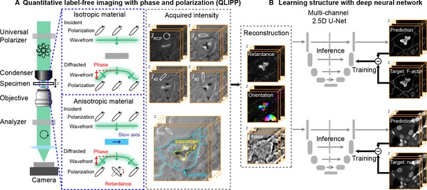
Measurements with QLIPP and analysis of structures with 2.5D U-Net.
(A) Light path of the microscope. Volumes of polarization-resolved images are acquired by illuminating the specimen with light of diverse polarization states. Polarization states are controlled using a liquid-crystal universal polarizer. Isotropic material’s optical path length variations cause changes in the wavefront (i.e., phase) of light that is measurable through defocused intensity stack. Anisotropic material not only changes the wavefront, but also changes the polarization of light depending on the degree of optical anisotropy (retardance) and orientation of anisotropy. Intensity Z-stacks of an example specimen, mouse kidney tissue, under five illumination polarization states ( are shown. The intensity variations that encode the reconstructed physical properties of isotropic and anisotropic material are illustrated in the stack I135. These polarization-resolved stacks are used to reconstruct (Materials and methods) the specimen’s retardance, slow-axis orientation, and phase. Slow-axis orientation at given voxel reports the axis in the focal plane along which the material is the densest and is represent by a color according to the half-wheel shown in inset. (B) Multi-channel, 2.5D U-Net model is trained to predict fluorescent structures from label-free measurements. In this example 3D distribution of F-actin and nuclei are predicted. During training, pairs of label-free images and fluorescence images are supplied as inputs and targets, respectively, to the U-Net model. The model is optimized by minimizing the difference between the model prediction and the target. During inference, only label-free images are used as input to the trained model to predict fluorescence images.
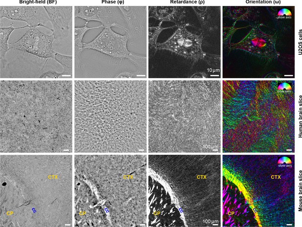
Complementary measurements of phase, retardance, and slow-axis orientation distinguish biological structures.
Brightfield (BF), phase (Φ), retardance (ρ), and slow-axis orientation (ω) images of U2OS cells, human brain tissue, and adult mouse brain tissue are shown. In orientation images, slow axis and retardance of the specimen are represented by color (hue) and brightness, respectively. In U2OS cells, chromatin, lipid droplets, membranous organelles, and cell boundaries are visible in phase image due to variations in density, while microtubule spindle, lipid droplets, and cell boundaries are visible due to their anisotropy. In the adult mouse brain slices, axon tracts are more visible in phase, retardance, and orientation images compared to brightfield images, with slow axis perpendicular to the direction of the bundles (cc: corpus callosum, CP: caudoputamen, CTX: cortex). Similar label-free contrast variations are observed in developing human brain tissue slice, but with less ordered tracts compared to the adult mouse brain due to the early age of the brain. The 3D stack of live U2OS cell was acquired with 63 × 1.47 NA oil objective and 0.9 NA illumination, whereas images of mouse and human brain tissue were acquired with 10 × 0.3 NA air objective and 0.2 NA of illumination.
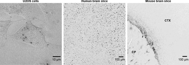
Degree of polarization (DOP) images for three specimens shown in Figure 2.
When the specimen does not exhibit multiple scattering or diattenuation, . The DOP decreases when the specimen exhibits multiple scattering and increases when the specimen exhibits diattenutation, that is, polarization-dependent absorption. The anatomical labels for the mouse brain slice are, cc: corpus callosum, CP: caudoputamen, CTX: cortex.
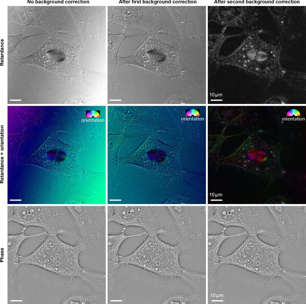
Effect of background correction methods on reconstructed retardance and phase of the U2OS cell.
When the specimen has intrinsically low retardance, background correction methods have a large impact on the reconstructed retardance and slow axis orientation. However, the background correction has no significant impact on phase reconstruction. (Left column) Reconstructions without background correction. (Middle column) Background-corrected reconstruction using an experimental images of empty region next to the cells (Right column) Background-corrected reconstruction using images estimated by fitting a very smooth surface to specimen image.
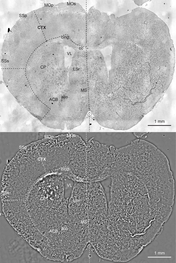
Comparison of brightfield image (top) with quantitative phase image (bottom) of a mouse brain slice.
The phase image reports density variations at higher contrast. These images are stitches of 48 fields of view and are substantially downsampled to reduce the size. This mouse brain section is a coronal section at around bregma 0.945 mm and is labeled according to Allen brain reference atlas (level 45) (Lein et al., 2007). ACB: nucleus accumbens, aco: anterior commissure, olfactory limb, cc: corpus callosum, cing: cingulum bundle, CTX: cortex, CP: caudoputamen, LSr: lateral septal nucleus, rostral part, MOp: primary motor cortex, MOs: secondary motor cortex, MS: medial septal nucleus, SSp: primary somatosensory area, SSs: supplemental somatosensory area, VL: lateral ventricle.
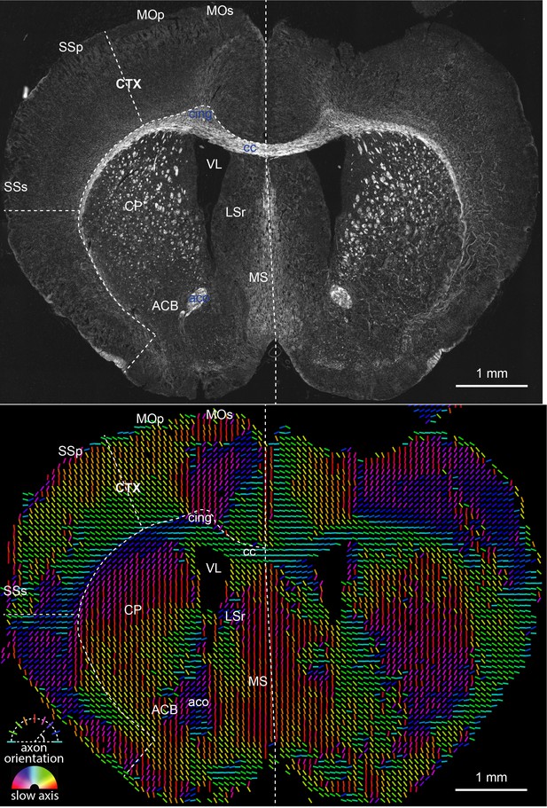
Retardance (top) and orientation (bottom) measurements of a mouse brain slice, which report structural anisotropy and axon orientation (in physical line orientation), respectively.
The color of the orientation line reports the slow axis orientation of the pixel. We needed to compress the measured dynamic range of retardance by using gamma correction (0.5) to visualize less anisotropic gray matter in the presence of highly anisotropic white matter. These images are stitches of 48 fields of view and are substantially downsampled to reduce size. The peak retardance is 50 nm.
Z-stacks of brightfield and phase images of U2OS cells.
The same field of view is shown in Figure 2.
Time-lapse of phase, retardance, and slow axis orientation in a dividing U2OS cell shows differences in density and anisotropy of organelles.
The same field of view is shown in Figure 2.
3D rendering of the time-lapse showing diverse structures color coded by their retardance and phase in U2OS cells shown in Figure 2.
Phase values from low to high are color-coded with magenta, cyan, and green, respectively. Retardance values are color-coded with yellow. With this pseudo-color scheme, cytoplasm appears in magenta, chromatin appears in magenta and changes to blue as it condenses to chromosomes, nucleoli appear in blue, lipid vesicles appear in green surrounded by yellow rings, and spindles appear in yellow .
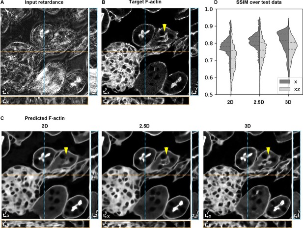
Accuracy of 3D prediction with 2D, 2.5D, and 3D U-Nets.
Orthogonal sections (XY - top, XZ - bottom, YZ - right) of a glomerulus and its surrounding tissue from the test set are shown depicting (A) retardance (input image), (B) experimental fluorescence of F-actin stain (target image), and (C) Predictions of F-actin (output images) using the retardance image as input with different U-Net architectures. (D) Violin plots of structral-similarty metric (SSIM) between images of predicted and target stain in XY and XZ planes. The horizontal dashed lines in the violin plots indicate 25th quartile, median, and 75th quartile of SSIM. The yellow triangle in C highlights a tubule structure, whose prediction can be seen to improve as the model has access to more information along Z. The same field of view is shown in Figure 3—video 1, Figure 3—video 2, and Figure 4—video 1.
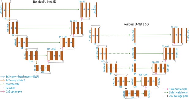
Schematic illustrating U-Net architectures.
Schematic of 2D U-Net model used for translating slice→slice and 2.5D U-Net model used for translating stack→slice. The 3D U-Net model used for translating stack→stack is similar to the 2D U-Net, but uses 3D convolutions instead of 2D and is four layers deep instead of 5 layers deep.
Z-stacks of brightfield, phase, retardance, and orientation images of mouse kidney tissue.
Through focus series showing 3D F-actin distribution in the test field of view shown in Figure 3.
We show F-actin distribution (labeled with phalloidin-AF568) acquired on a confocal microscope (target), as well as predicted from 2D, 2.5D, and 3D models trained to translate retardance distribution into fluorescence distributions.
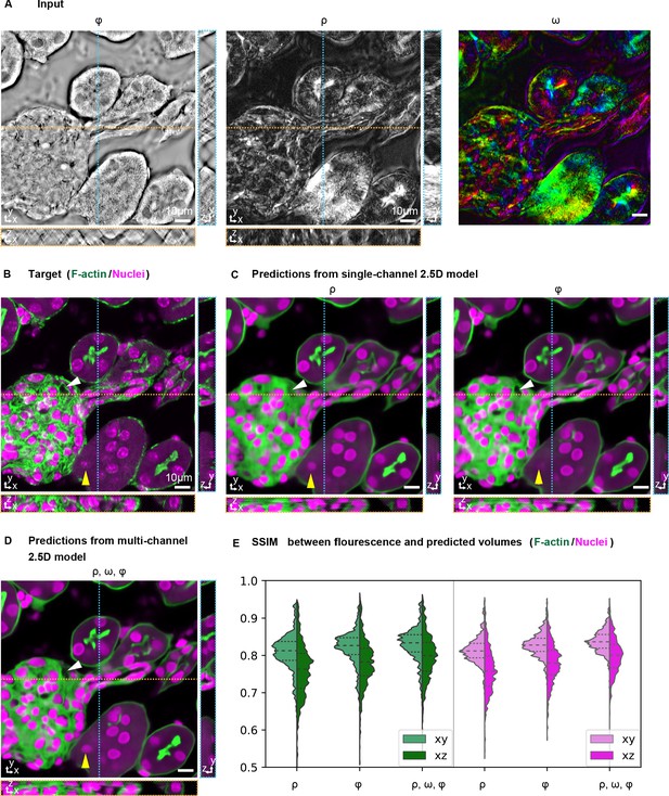
Prediction accuracy improves with multiple label-free contrasts as inputs.
3D predictions of ordered F-actin and nuclei from different combinations of label-free contrasts using the 2.5D U-Net model. (A) Label-free measurements used as inputs for model training: retardance (ρ), phase (Φ), and slow axis orientation (ω). (B) The corresponding 3D volume showing the target fluorescent stains. Phalloidin-labeled F-actin in shown green and DAPI labeled nuclei is shown in magenta. (C) F-actin and nuclei predicted with single channel models trained on retardance (ρ) and phase (Φ) alone are shown. (D) F-actin and nuclei predicted with multi-channel models trained with the combined input of retardance, orientation, and phase. The yellow triangle and white triangle point out structures missing in predicted F-actin and nuclei distributions when only one channel is used as an input, but predicted when all channels are used. (E) Violin plots of structral-similarty metric (SSIM) between images of predicted and experimental stain in XY and XZ planes. The horizontal dashed lines indicate 25th quartile, median, and 75th quartile of SSIM. The 3D label-free inputs used for prediction are shown in Figure 3—video 1.
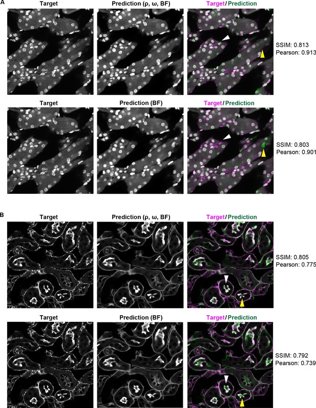
Pearson correlation and SSIM are insensitive to small structural differences in the images.
(A) DAPI labeled nuclei predicted by the model trained with combined input of retardance (ρ), orientation (ω), and brightfield and with brihgtfield alone (B) F-actin predicted by the model trained with combined input of retardance (ρ), orientation (ω), and brightfield and with brihgtfield alone. The differences in prediction SSIM and Pearson correlation between the multi-contrast and single contrast models are relatively small (∼0.01) despite the perceivable structural differences shown in the images (indicated by the yellow triangle and white triangle). These structural differences such as missing/spurious nuclei and separate/connected F-actin structures may affect the interpretation of the experimental results depending on the context.
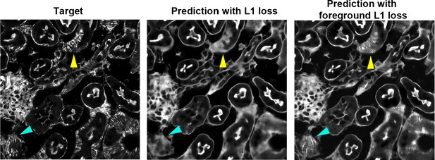
Fine structural features are better predicted with foreground loss.
F-actin in the mouse kidney slice predicted by the model trained with regular L1 loss (middle) and foreground only L1 loss (right). F-actin was predicted from combined input of retardance (ρ), orientation (ω), and brightfield. Fine F-actin bundles are not visible in prediction with regular L1 loss but visible in prediction with foreground L1 loss.
Through focus series showing 3D F-actin and nuclei distribution in the test field of view shown in Figure 4.
We show overlays of F-actin (phalloidin-AF568) distribution in green and nuclei (DAPI) distribution in magenta DAPI as acquired on confocal (target) and as predicted from models. Predictions were obtained from 2.5D models trained on retardance alone, phase alone, and on combination of retardance, orientation, phase
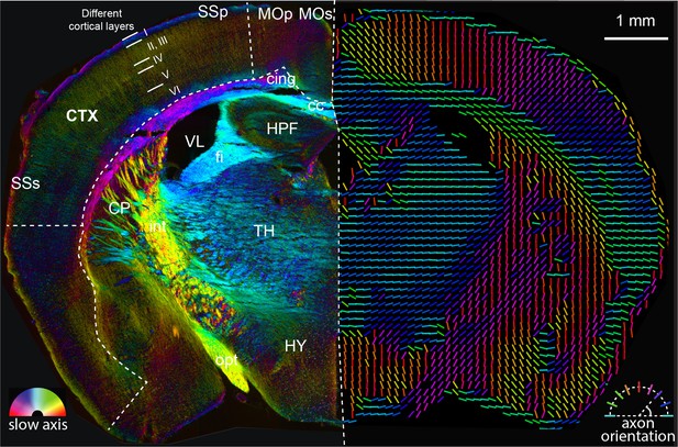
Analysis of anatomy and axon orientation of an adult mouse brain tissue with QLIPP.
The retardance and orientation measurements are rendered with two approaches in opposing hemispheres of the mouse brain, respectively. In the left panel, the slow-axis orientation is displayed with color (hue) and the retardance is displayed with brightness as shown by the color legend in bottom-left. In the right panel, the colored lines represent fast axis and the direction of the axon bundles in the brain. The color of the line still represents the slow-axis orientation as shown by color legend in bottom-right. Different cortical layers and anatomical structures are visible through this measurements. This mouse brain section is a coronal section at around bregma −1.355 mm and is labeled according to Allen brain reference atlas (level 68) (Lein et al., 2007). cc: corpus callosum, cing: cingulum bundle, CTX: cortex, CP: caudoputamen, fi: fimbria, HPF: hippocampal formation, HY: hypothalamus, int: internal capsule, MOp: primary motor cortex, MOs: secondary motor cortex, opt: optic tract, SSp: primary somatosensory area, SSs: supplemental somatosensory area, TH: thalamus, VL: lateral ventricle.
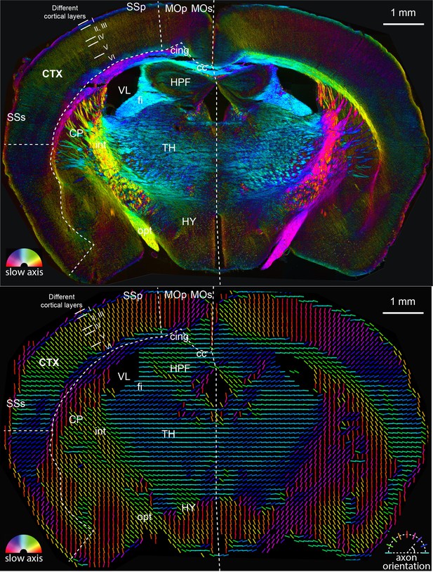
The full-size mouse brain images of two rendering approaches shown in Figure 5.
In the top panel, the slow-axis orientation is displayed with color (hue) and the retardance is displayed with brightness as shown by the color legend in bottom-left. In the bottom panel, the colored lines represent fast axis and the direction of the axon bundles in the brain. The color of the line still represents the slow-axis orientation as shown by color legend in bottom-right.
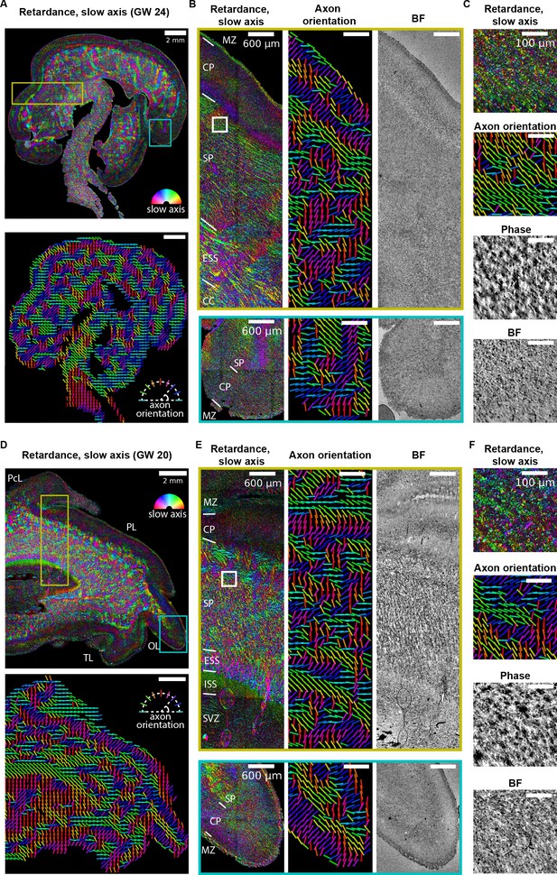
Label-free mapping of axon tracts in developing human brain tissue section.
(A) (top) Stitched image of retardance and slow axis orientation of a gestational week 24 (GW24) brain section from the test set. The slow axis orientation is encoded by color as shown by the legend. (Bottom) Axon orientation indicated by the lines. (B) Zoom-ins of retardace + slow axis, axon orientation, and brightfield at brain regions indicated by the yellow and cyan boxes in (A). (C) Zoom-ins of label-free images at brain regions indicated by the white box in (B) (D–F) Same as (A–C), but for GW20 sample. MZ: marginal zone; CP: cortical plate; SP: subplate; ESS: external sagittal stratum; ISS: internal sagittal stratum; CC: corpus callosum; SVZ: subventricular zone; PcL: paracentral lobule PL: parietal lobe; OL: occipital lobe; TL: temporal lobe. Anatomical regions in (B, D, and E) are identified by referencing to developing human brain atlas (Bayer and Altman, 2003).
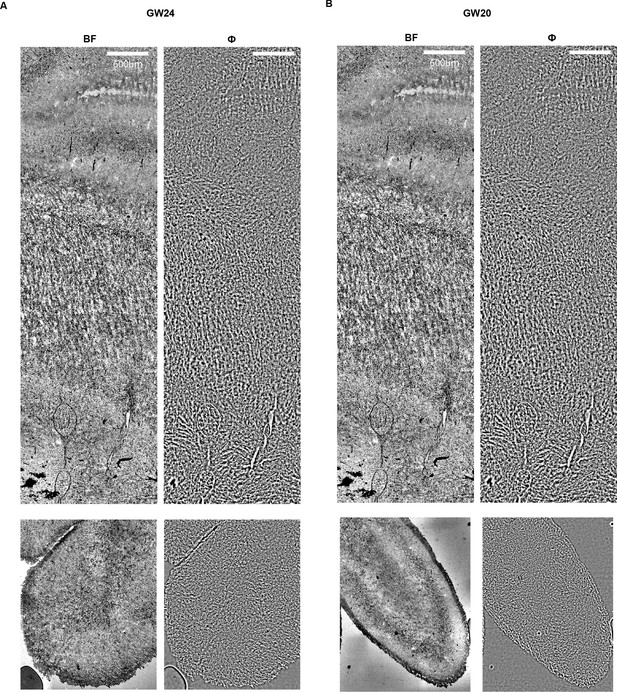
Brightfield and phase images of human brain sections.
Images from the same field of view shown in Figure 4 for (A) GW24 and (B) GW20. Scale bars: (A–C) .
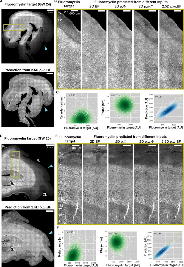
Prediction of myelination in developing human brain from QLIPP data and rescue of inconsistent labeling.
(A) Stitched image of experimental FluoroMyelin stain of the same (GW24) brain section from the test set (top) and FluoroMyelin stain predicted from retardance, slow axis orientation, brightfield by the 2.5D model (bottom). The cyan arrow head indicates large staining artifacts in the experimental FluoroMyelin stain but rescued in model prediction. (B) Zoom-ins of experimental and predicted FluoroMyelin stain using different models at brain regions indicated by the yellow box in (A) rotated by 90 degrees. From left to right: experimental FluoroMyelin stain; prediction from brightfield using 2D model; prediction from retardance and phase using 2D model; prediction from retardance, phase, and orientation using 2D model; prediction from retardance, brightfield, and orientation using 2.5D model. (C) From region shown in (B) we show scatter plot and Pearson correlation of target FluoroMyelin intensity v.s. retardace (left), phase (middle), FluoroMyelin intensity predicted from retardance, brightfield, and orientation using 2.5D model (right). Yellow dashed line indicates the function y = x. (D–F) Same as (A–C), but for GW20 sample. MZ: marginal zone; CP: cortical plate; SP: subplate; ESS: external sagittal stratum; ISS: internal sagittal stratum; CC: corpus callosum; SVZ: subventricular zone; PcL: paracentral lobule PL: parietal lobe; OL: occipital lobe; TL: temporal lobe.
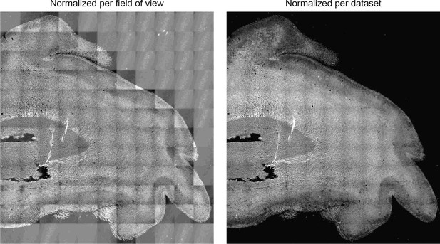
Normalizing training data per dataset yields prediction with correct dynamic range of intensity.
Predictions of FluoroMyelin in GW20 human brain tissue slice with training data normalized per field of view (left) and across dataset (right).
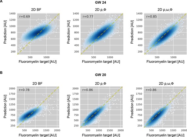
Model predicted FluoroMyelin intensity becomes more accurate as more label-free channels are included as input.
Scatter plot and Pearson correlation of target FluoroMyelin intensity v.s. model predicted FluoroMyelin intensity for region shown in Figure 5B. for (A) GW24 and (B) GW20. We show prediction from brightfield using 2D model (left); prediction from retardance and phase using 2D model (middle); prediction from retardance, phase, and orientation using 2D model (right).
Tables
Accuracy of 3D prediction of F-actin from retardance stack using different neural networks.
Above table lists median values of the Pearson correlation (r) and structural similarity index (SSIM) between prediction and target F-actin volumes. We report accuracy metrics for Slice→Slice (2D) ,Stack→Slice (2.5D), and Stack→Stack (3D) models trained to predict F-actin from retardance using Mean Absolute Error (MAE or L1) loss. We segmented target images with a Rosin threshold to discard tiles that mostly contained background pixels. To dissect the differences in prediction accuracy along and perpendicular to the focal plane, we computed (Materials and methods) test metrics separately over XY slices (rxy, SSIMxy) and XZ slices (rxy, SSIMxz) of the test volumes, as well as over entire test volumes (rxyz, SSIMxyz). Best performing model according to each metric is displayed in bold.
| Translation model | Input(s) | rxy | rxz | rxyz | SSIMxy | SSIMxz | SSIMxyz |
|---|---|---|---|---|---|---|---|
| Slice→Slice (2D) | ρ | 0.82 | 0.79 | 0.83 | 0.78 | 0.71 | 0.78 |
| Stack→Slice (2.5D, ) | ρ | 0.85 | 0.83 | 0.86 | 0.80 | 0.75 | 0.81 |
| Stack→Slice (2.5D, ) | ρ | 0.86 | 0.84 | 0.87 | 0.81 | 0.76 | 0.82 |
| Stack→Slice (2.5D, ) | ρ | 0.87 | 0.85 | 0.87 | 0.82 | 0.77 | 0.83 |
| Stack→Stack (3D, ) | ρ | 0.86 | 0.84 | 0.86 | 0.82 | 0.76 | 0.85 |
Accuracy of prediction of F-actin in mouse kidney tissue as a function of input channels.
Median values of the Pearson correlation (r) and structural similarity index (SSIM) between predicted and target volumes of F-actin. We evaluated combinations of brightfield (BF), phase (Φ), retardance (ρ), orientation x (ωx), and orientation y (ωy), as input. Model training conditions and computation of test metrics is described in Table 1.
| Translation model | Input(s) | rxy | rxz | rxyz | SSIMxy | SSIMxz | SSIMxyz |
|---|---|---|---|---|---|---|---|
| Stack→Slice (2.5D, ) | ρ | 0.86 | 0.84 | 0.87 | 0.81 | 0.76 | 0.82 |
| BF | 0.86 | 0.84 | 0.86 | 0.82 | 0.77 | 0.83 | |
| Φ | 0.87 | 0.85 | 0.88 | 0.83 | 0.78 | 0.84 | |
| Φ, ρ, ωx, ωy | 0.88 | 0.87 | 0.89 | 0.83 | 0.80 | 0.85 | |
| BF, ρ, ωx, ωy | 0.88 | 0.87 | 0.89 | 0.83 | 0.79 | 0.85 |
Accuracy of prediction of nuclei in mouse kidney tissue.
Median values of the Pearson correlation (r) and structural similarity index (SSIM) between predicted and target volumes of nuclei. See Table 2 for description.
| Translation model | Input(s) | rxy | rxz | rxyz | SSIMxy | SSIMxz | SSIMxyz |
|---|---|---|---|---|---|---|---|
| Stack→Slice (2.5D, ) | ρ | 0.84 | 0.85 | 0.85 | 0.81 | 0.76 | 0.82 |
| BF | 0.87 | 0.88 | 0.87 | 0.82 | 0.77 | 0.84 | |
| Φ | 0.88 | 0.88 | 0.88 | 0.83 | 0.78 | 0.85 | |
| Φ, ρ, ωx, ωy | 0.89 | 0.89 | 0.89 | 0.84 | 0.80 | 0.86 | |
| BF, ρ, ωx, ωy | 0.89 | 0.90 | 0.89 | 0.84 | 0.80 | 0.86 |
Accuracy of prediction of FluoroMyelin in human brain tissue slices across two developmental points (GW20 and GW24).
Median values of the Pearson correlation (r) and structural similarity index (SSIM) between predictions of image translation models and target fluorescence. We evaluated combinations of retardance (ρ), orientation x (ωx), orientation y (ωy), phase (Φ), and brightfield (BF) as inputs. These metrics are computed over 15% of the fields of view from two GW20 datasets and two GW24 test datasets. The 2D models take ∼ 4 hours to converge, whereas 2.5D models take ∼ 64 hours to converge.
| Translation model | Input(s) | rxy | SSIMxy |
|---|---|---|---|
| Slice→Slice (2D) | BF | 0.72 | 0.71 |
| ρ, Φ | 0.82 | 0.82 | |
| ρ, ωx, ωy, Φ | 0.86 | 0.85 | |
| Stack→Slice (2.5D, ) | BF, ρ, ωx, ωy | 0.87 | 0.85 |
| Reagent type (species) or resource | Designation | Source or reference | Identifiers | Additional information |
|---|---|---|---|---|
| biological sample (M. musculus) | mouse kidney tissue section | Thermo-Fisher Scientific | Cat. # F24630 | |
| biological sample (M. musculus) | mouse brain tissue section | this paper | mouse line maintained in M. Han lab, see Specimen preparation in Materials and methods | |
| biological sample (H. sapiens) | developing human brain tissue section | this paper | archival tissue stored in T. Nowakowski lab, see Specimen preparation in Materials and methods | |
| chemical compound, drug | FluoroMyelin | Thermo-Fisher Scientific | Cat. # F34652 | |
| software, algorithm | reconstruction algorithms | https://github.com/mehta-lab/reconstruct-order | ||
| software, algorithm | 2.5 U-Net | https://github.com/czbiohub/microDL | ||
| software, algorithm | Micro-Manager 1.4.22 | https://micro-manager.org/ | RRID:SCR_016865 | |
| software, algorithm | OpenPolScope | https://openpolscope.org/ |


