A taxonomy of seizure dynamotypes
- Aix Marseille Univ, Inserm, INS, Institut de Neurosciences des Systèmes, Marseille, France, France
- Department of Biomedical Engineering, BioInterfaces Institute, University of Michigan, United States
- Graeme Clark Institute, The University of Melbourne, Australia
- Department of Medicine, St. Vincent's Hospital, The University of Melbourne, Australia
- Faculty of Information Technology, Monash University, Australia
- Department of Epilepsy, Movement Disorders and Physiology, Kyoto University Graduate School of Medicine, Japan
- Epilepsy Center, Medical Center – University of Freiburg, Germany
- Faculty of Medicine, University of Freiburg, Germany
- Center for Basics in NeuroModulation (NeuroModul Basics), Epilepsy Center, Medical Center - University of Freiburg, Germany
- Department of Neurology, University of Michigan, United States
Figures
Figure 1
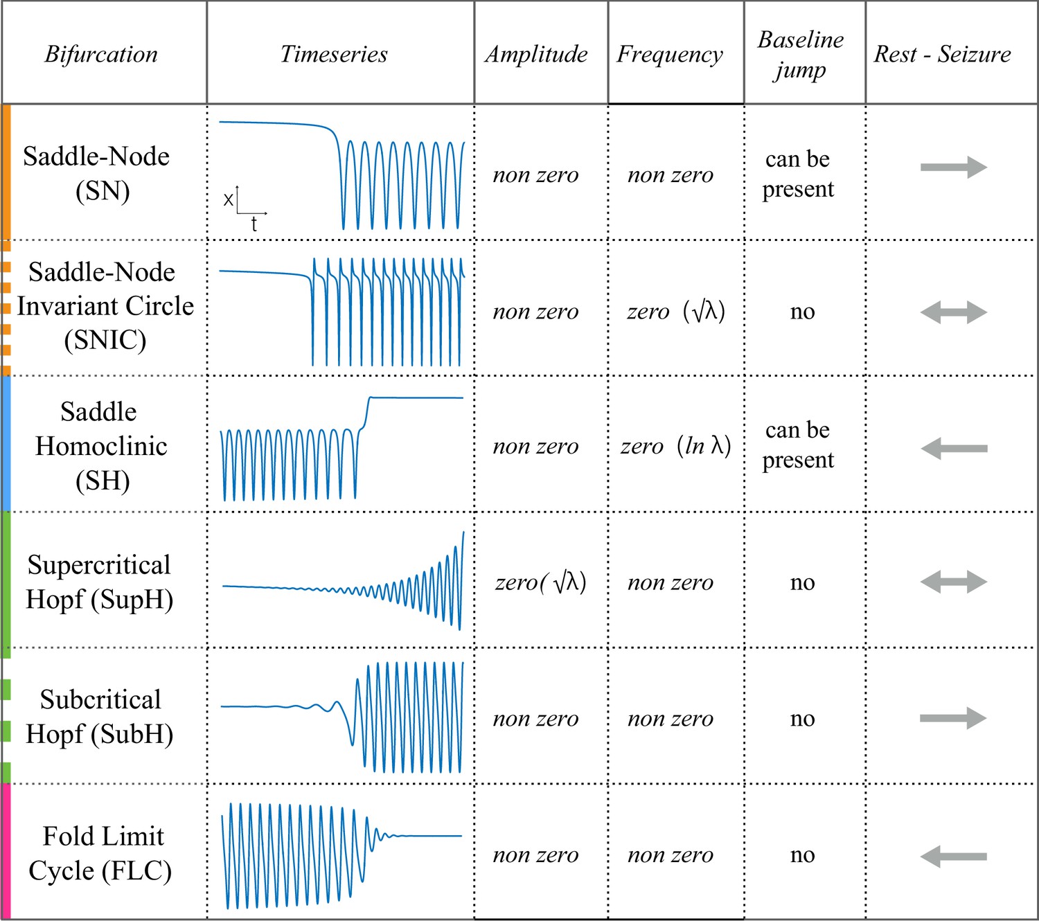
Scaling-laws of bifurcations.
Six bifurcations are responsible for the transition from rest to seizure and vice-versa. For each bifurcation we report: name and abbreviation; an example of timeseries; whether the amplitude or frequency of the oscillations goes to zero at the bifurcation point, and if they do how they change as a function of the distance to the bifurcation point (λ); whether the baseline of the signal shows a baseline shift; and if the bifurcation can be used to start (→) or stop (←) a seizure or both (←→).
Figure 2
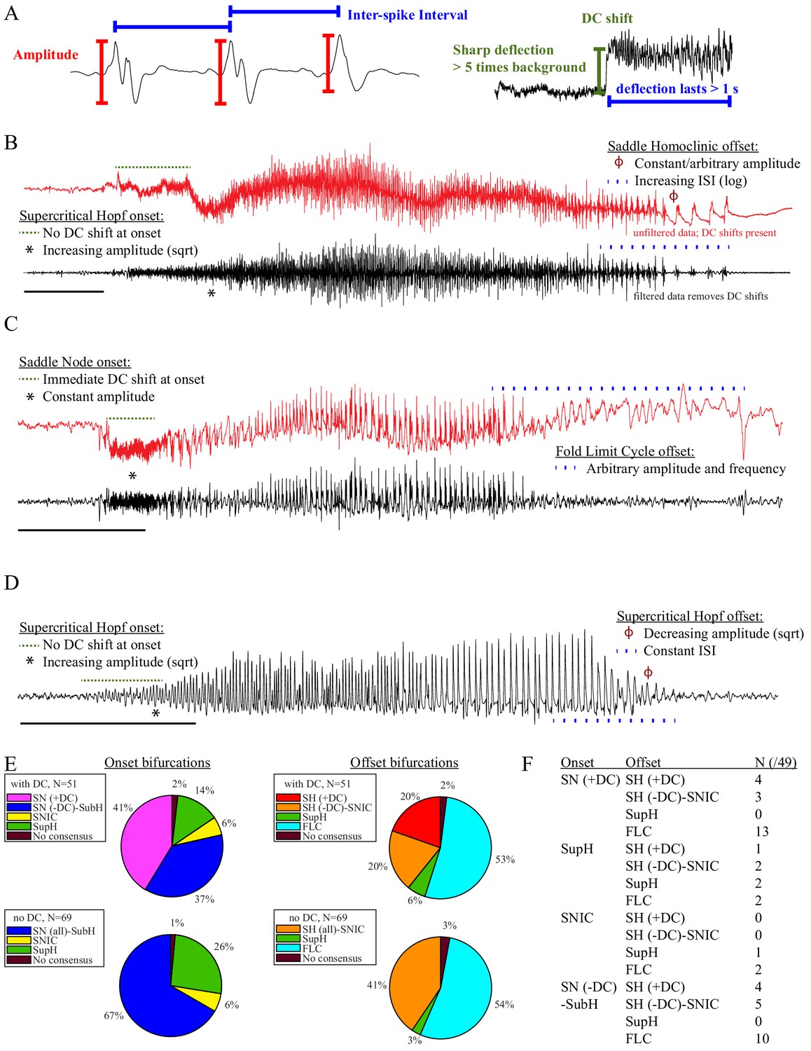
Seizure dynamics taxonomy.
(A) Interspike intervals (ISI) and peak-to-peak amplitude were measured for every spike during seizures. DC shift was defined as sharp (<0.5 s) deflections that rise >5 times the background variance and persist for at least 1 s. (B) DC-coupled (red) and high-pass filtered (black) data of a seizure shows SupH onset and SH offset. (C) SN onset characterized by DC shift at onset. Ambiguous seizure offsets were included in the analysis as FLC. (D) SupH onset and offset. Although this patient did not have DC-coupled recordings, the amplitude scaling is clearly most consistent with SupH. Scale bars: 10 s. (E) Final results for all onset and offset bifurcations tested. All four bifurcation types were present. (F) Final taxonomy of the 39 patients with onset+offset classifications. In patients with DC recordings, SH offset was sometimes distinguishable from SNIC.
Figure 3
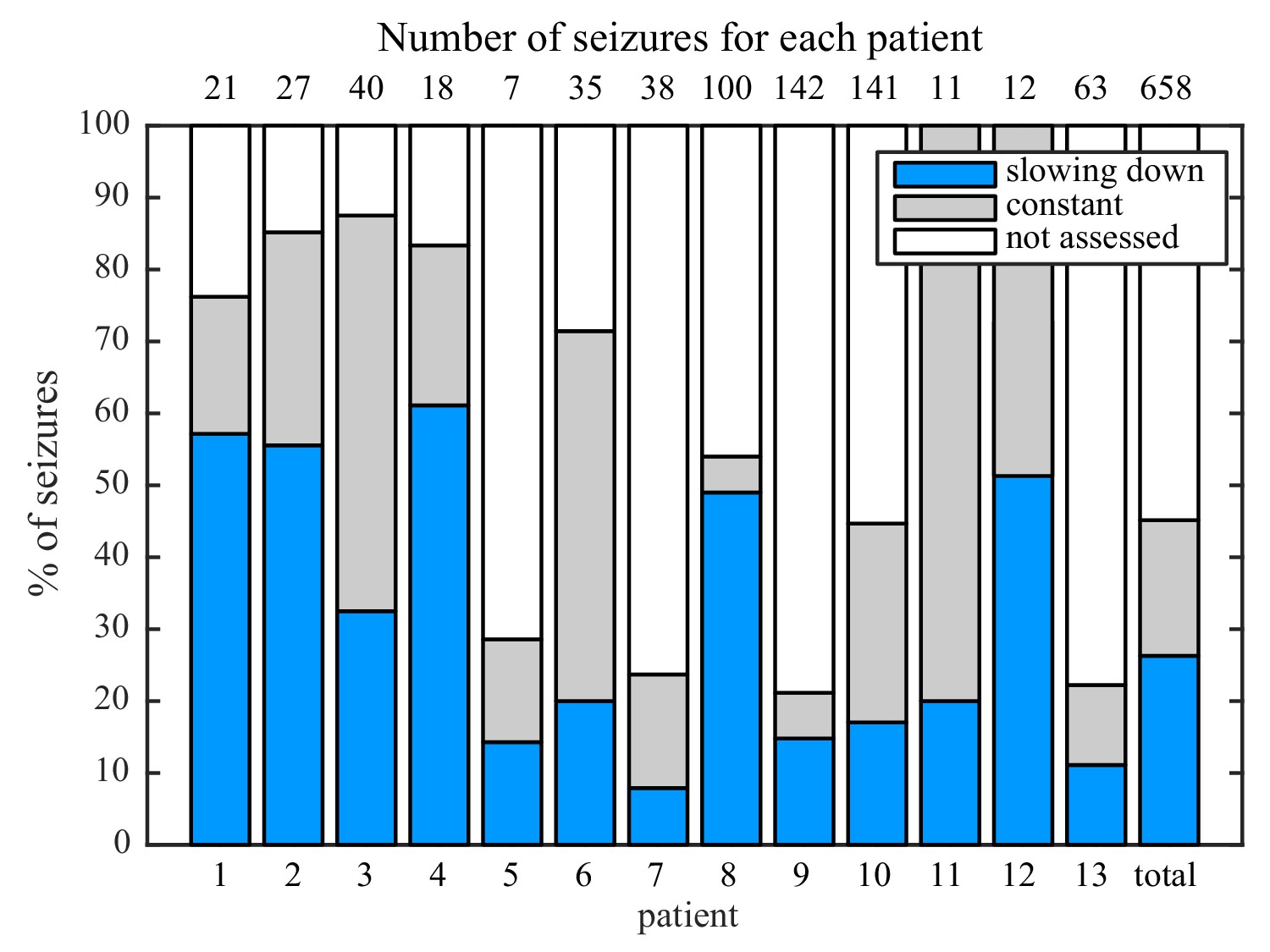
Manual classification of seizures from long-term intracranial recordings.
As a conservative analysis, colored bars show seizures with unequivocal slowing-down (blue) or constant (grey) scaling, demonstrating that all 13 patients had both types of seizure offset. Additional seizures that had more difficult classification (white) were not needed for this analysis, as each patient had already demonstrated both offset types.
Figure 4
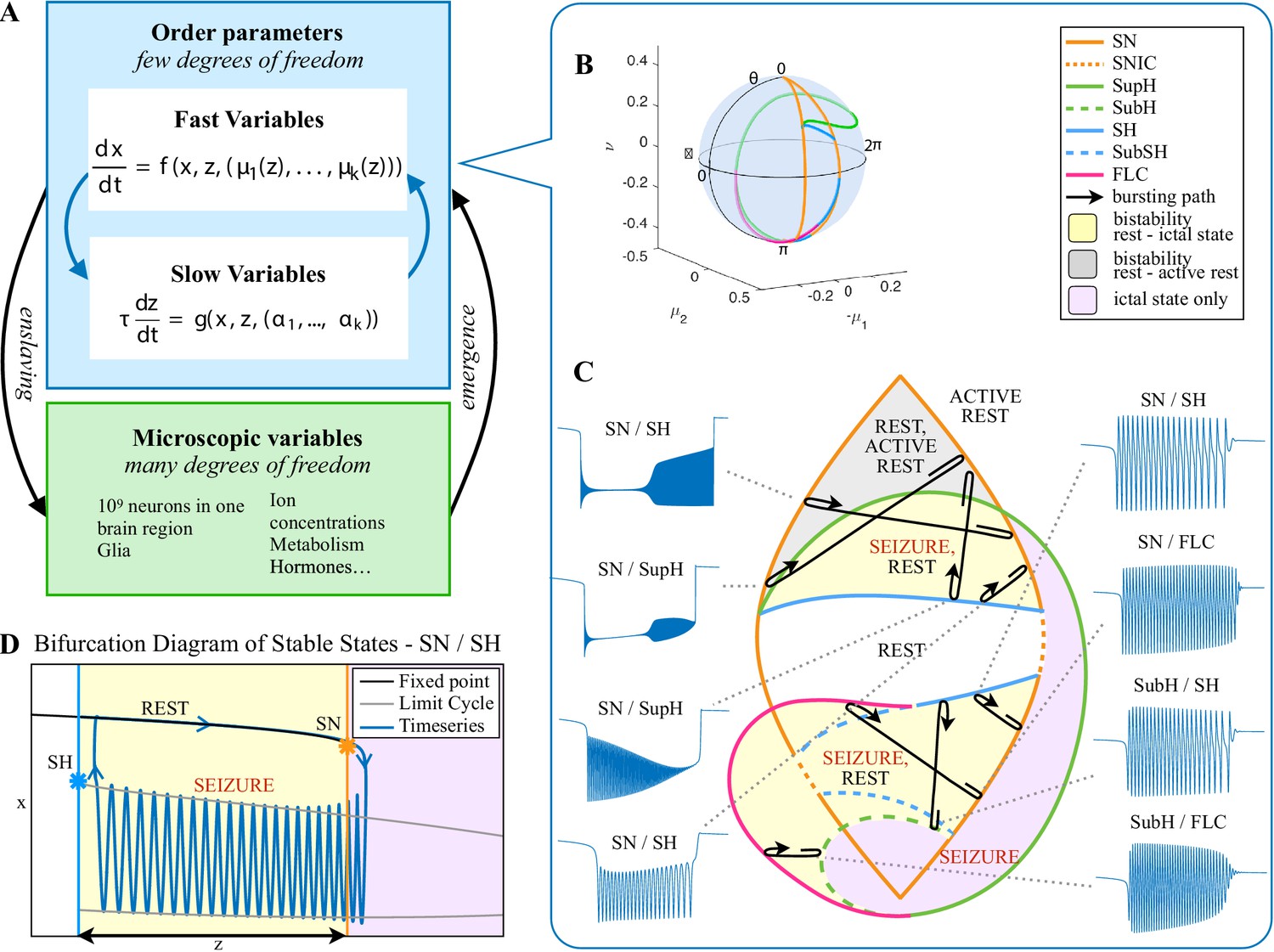
Modeling seizures.
(A) During a seizure the microscopic variables, which compose a brain region, organize so that the emergent global activity can be described by a few collective variables. These collective variables, on the other hand, act on the microscopic variables, ‘enslaving’ them. (B) The fast variables can be in different states depending on the values of the parameters. In our model, we have three parameters ; however, the relevant dynamics occurs on a sphere with fixed radius. We thus consider the two-parameter spherical surface that can be sketched with a flat map as shown in C. (C) Bifurcation curves divide the map in regions where different states are possible: healthy state (white), ictal state (violet), coexistence between healthy and ictal states (yellow), coexistence between healthy and ‘active’ rest (a non-oscillatory state with a different baseline than the healthy state (gray)). When a seizure starts because the system crosses an onset bifurcation, the slow variable enables movement along the black arrow (a path in the map) to bring the system back to rest. Note that in this model, the system alternates between the resting and seizing states within the bistability regions. The shape of the arrow is meant to better show the trajectory followed by the system, however movement in the model occurs back and forth along the same curve. Insets show example of timeseries for different paths. SubSH: Subcritical Saddle Homoclinic, an unstable limit cycle that occupies a small portion of the map but is incapable of starting/stopping seizures, and thus is not included in Figure 1 nor the rest of the analysis. (D) An expanded view of one trajectory followed in C. The path (double arrow) represents movement from resting to seizure state and back by crossing the bifurcations, which in this case are SN and SH. This activity forms a seizure in the time series. The resting state is represented by a black line (fixed point), the minimum and maximum of the amplitude of the seizure (limit cycle) by gray lines.
Figure 5
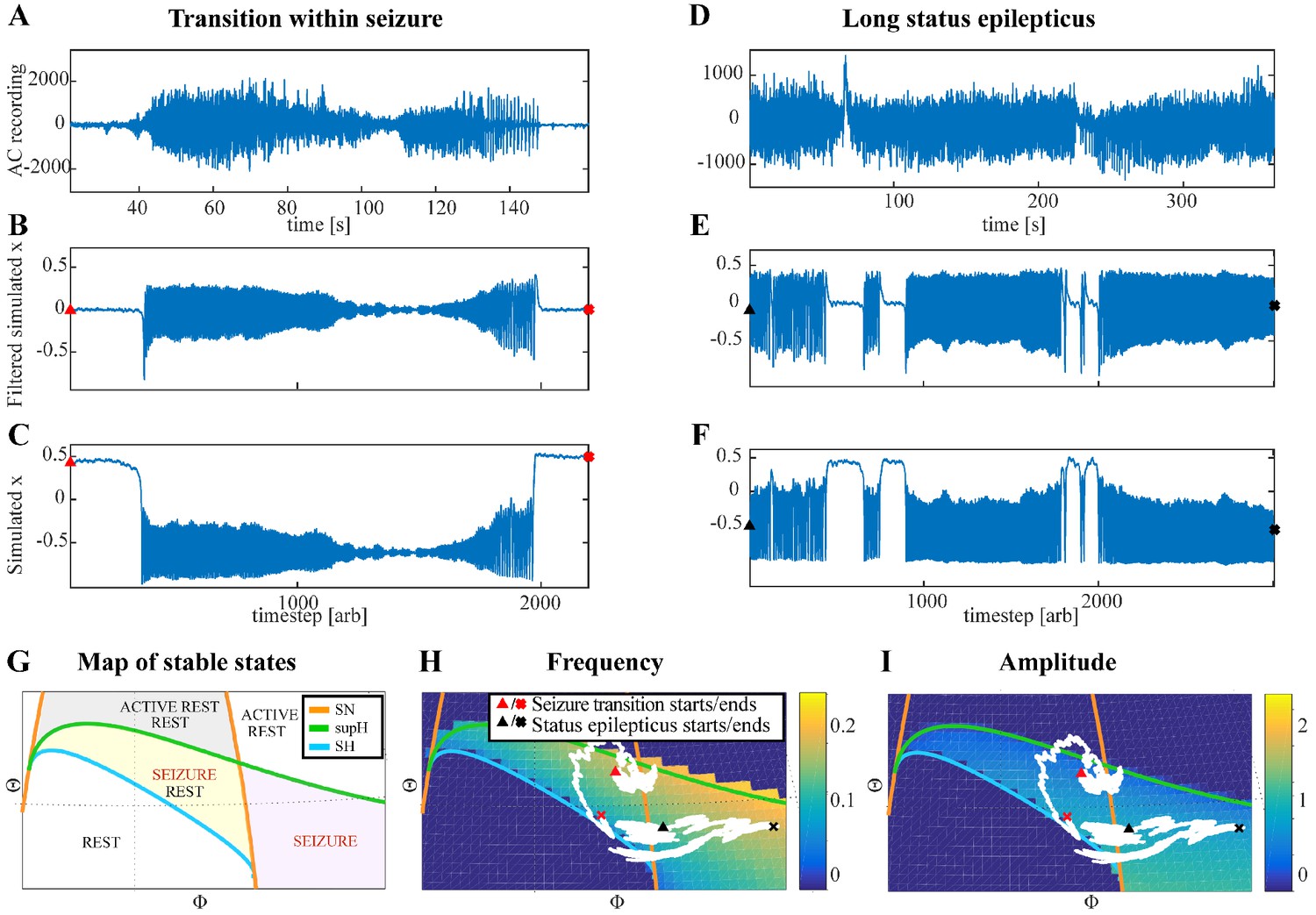
Fluctuations in the ultra-slow modulation of the path causes changes in the dynamics of the seizure.
(A) A recording in which the seizure begins to go toward a SupH offset (square-root decreasing amplitude), but the amplitude increases again and the final offset is SH. (B) A portion of the simulation of the model in Saggio et al., 2017 done to reproduce the dynamics observed in the recording. This timeseries is high pass filtered to simulate the effect of AC recordings. The non-filtered simulation is shown in (C). (D) A portion of a long status epilepticus recorded in one patient. The status epilepticus was characterized by transitions in the dynamics (such as at 70 s and 230 s). (E) High-pass filtered, and (F) unfiltered portion of model data simulating the behavior in D. (G) A zoomed, flattened projection of the map in Figure 4B (see Appendix II, IV), for reference in H-I. (H,I) Amplitude and frequency maps showing trajectories (white) of the modelled seizures in C,F. The seizure from C begins (red triangle) and naturally moves upwards toward the supH bifurcation, but a change in the ultraslow drift prior to termination pushes the system downward, changing the offset from SupH to SH. Conversely, the seizure from F begins (black triangle) and repeatedly moves towards the SH termination due to the ultraslow drift, but is pushed back into the seizure regime repeatedly by high levels of noise, which overrides the role of the slow variable in terminating the seizure.
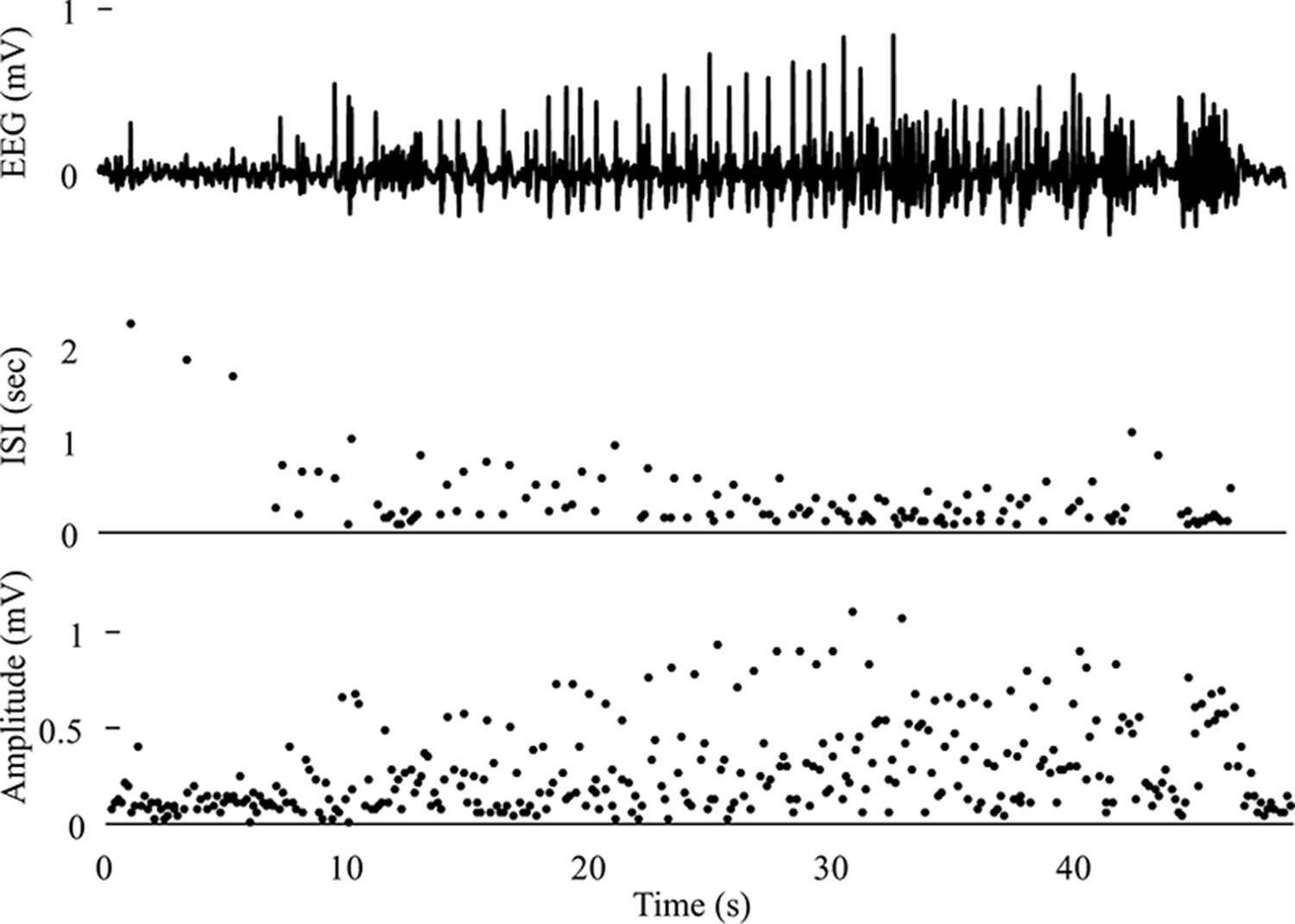
Appendix 1—figure 1
Saddle Node Onset DC-coupled recordings (green, top) show DC shift that occurs immediately upon seizure onset.
To determine spike amplitudes and ISI, data must be high-pass filtered (black). Those filtered data are then used to identify the spikes (red circles) for analysis. The interspike intervals (ISI, middle) and amplitude (bottom) of each spike are then plotted versus time since seizure onset for visual analysis and curve fitting. The seizure begins with fast 20 Hz firing at arbitrary amplitude for over 5 s. This is followed by changing amplitude, irregular firing, and then clonic bursting, but those are clearly after the initial onset. The combination of arbitrary amplitude, ISI, and DC shift is consistent with Saddle Node. Onset Classification: DC shift: yes, therefore SN onset. All three reviewers agreed. Offset Classification:57640 This is an example of a challenging offset. Analysis is uncertain because seizure offset time is unclear (is it when the fast spikes stop, when the slower oscillations stop, when the low voltage fast activity stops, or when the large final spike occurs?). Thus, the method is uncertain. DC shift: no. Amplitude decreasing: uncertain. ISI increasing: uncertain. This offset is ambiguous and reviewers were unable to reach consensus. One reviewer felt the high amplitude spiking fit with increasing ISI (SH or SNIC). Another felt it should be FLC because of the arbitrary patterns. Another was uncertain how to score given the ambiguity of seizure offset. It was listed as ‘no consensus’.
Appendix 1—figure 2
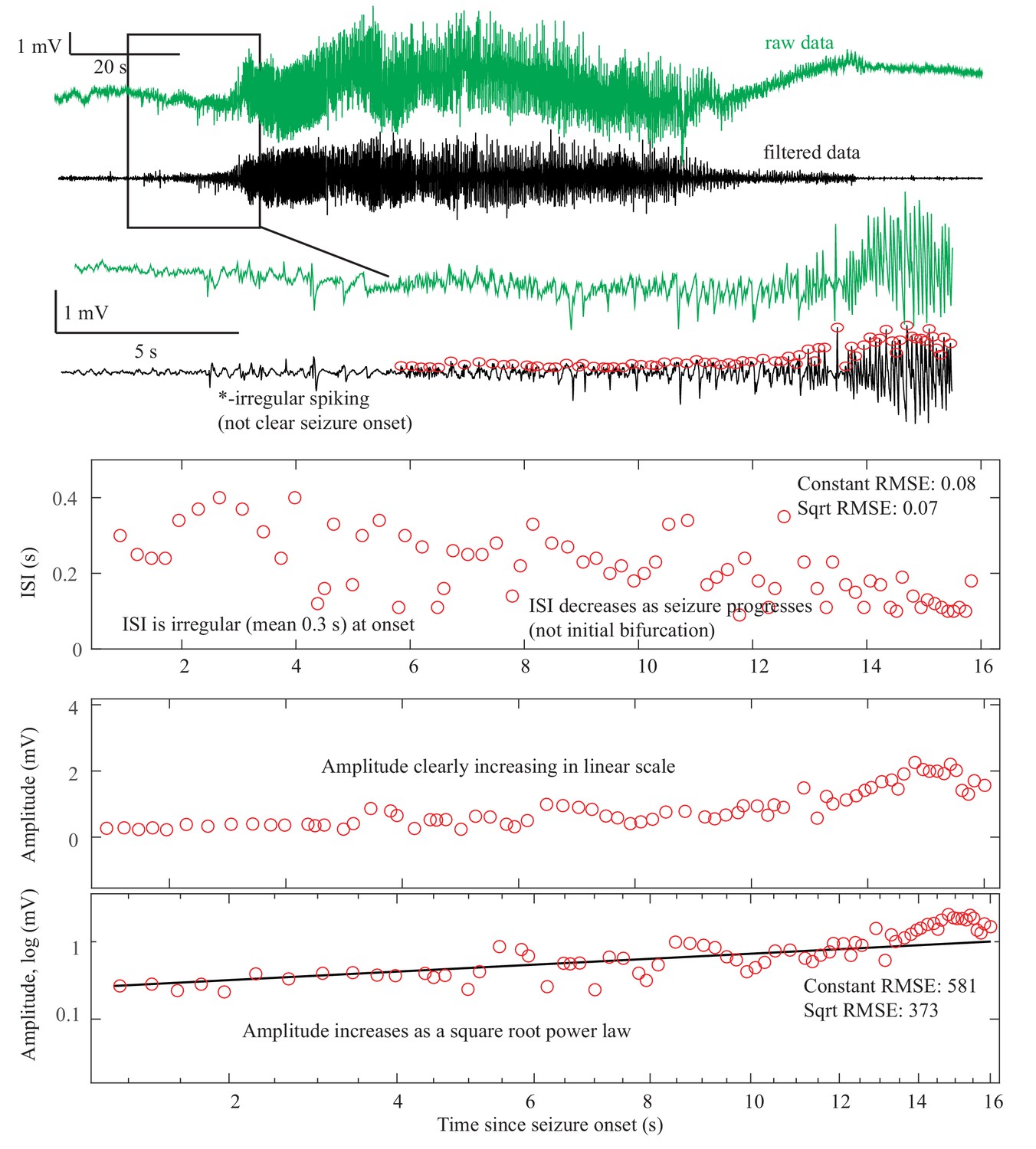
Supercritical Hopf Onset DC-coupled recordings (green, top) do not have a DC shift at onset.
The ISI is arbitrary at onset, then after 10 s starts to decrease (middle). This irregular spiking prior to the seizure (*) is not part of a clear seizure onset, does not conform to any initial bifurcation, and thus was not chosen as the unequivocal seizure onset. The sustained spiking that begins at 8 s, however, follows the SupH dynamics very well. Amplitude shows steady increase in linear scale, which appears as a straight light in loglog plots, consistent with a square root power law (loglog plot). This seizure is most consistent with SupH due to the amplitude scaling. Onset Classification: This onset is somewhat challenging because there was some disagreement about when the seizure started. A more straightforward SupH onset is seen in Figure 2 and Appendix 1—figure 8. In this case, two reviewers felt the irregular spiking was not a sustained start of the seizure and potentially was just preictal. One reviewer thought it could be the start and the seizure might be an arbitrary pattern (SubH or SN (-DC)). After discussion, reviewers agreed that the primary sustained pattern was increasing amplitude. Final analysis—DC shift: no. Amplitude increasing: yes, therefore SupH onset, but with note made of irregular spiking at seizure onset of uncertain significance. Offset Classification: This offset is difficult because there is decreasing amplitude like the onset, but then a persistent low voltage fast activity. DC shift: no. Amplitude decreasing: There was disagreement about whether the decrease comprised the final dynamotype of the seizure terminus, or if the low voltage fast activity that persisted at the end was a separate pattern. ISI increasing: no. Thus there was disagreement about whether this should be a SupH or FLC: there is a decreasing amplitude similar to the SupH onset pattern, followed by 15 s of constant ISI low voltage spiking.
Appendix 1—figure 3
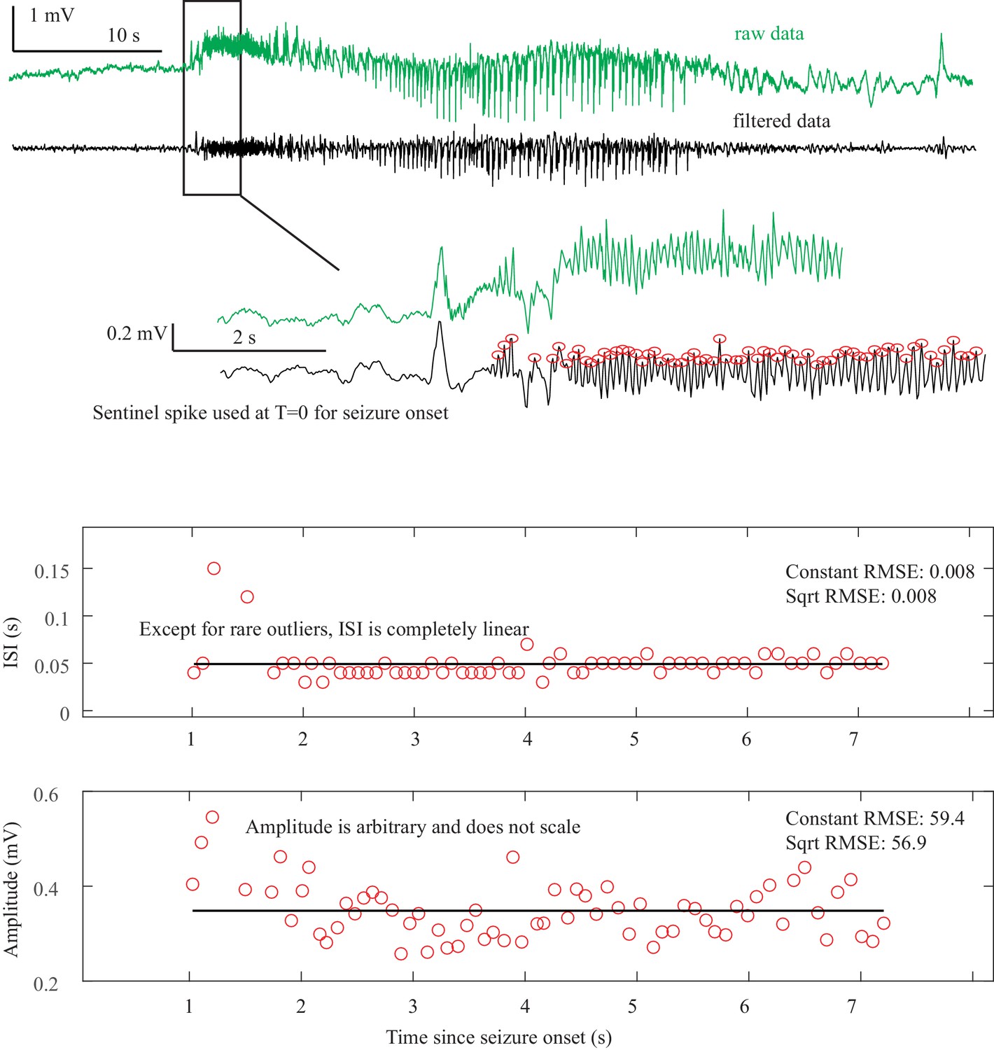
SNIC Onset. The seizure begins at some point after a sentinel spike.
The true starting time of this seizure is debatable, as there are three spike-waves with large ISI and amplitude but they do not persist. At 3.9 s after the sentinel spike (*) there is a fourth spike wave that leads into the unequivocal seizure onset, with accelerating frequency until 5 s. Whether one chooses T = 0 or T = 3.9 as the starting time can change the determination. At 3.9 s, the pattern starts with high amplitude spike waves that accelerate in frequency, characteristic of the SNIC. At 0 s, there was uncertainty whether the initial spike waves should be treated like a SNIC with a pause, or an arbitrary pattern. Spike wave discharges were present in both patients that we classified as SNIC, but are not a requirement. In this case, visual inspection was more reliable than fitting equations to make the determination because seizure onset was irregular. Onset Classification: DC shift: no. Amplitude scaling: no. ISI decreasing: yes, therefore a SNIC. However, there was concern that by starting at T = 0 this could be arbitrary rather than decreasing. After discussion it was felt this was most consistent with SNIC, as it appears to have accelerating ISI with a pause, rather than a truly arbitrary pattern. However, only 2/3 reviewers agreed. Offset Classification: DC shift: no. Amplitude or ISI scaling: no. This was classified as FLC. It has irregular gaps during the seizure that are not well described by the basic dynamotypes.
Appendix 1—figure 4
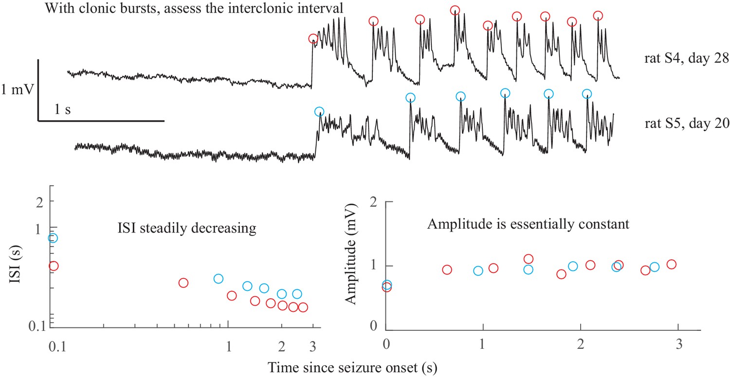
SNIC Onset in rats. There were no unequivocal examples of SNIC onset in our human data.
However, our group recently published data from the tetanus toxin model in rats that has excellent SNIC onsets (Crisp et al., 2020). Shown are data from two rats, which were shown in Figure 5 of that paper (see that work for details on experimental procedures). Both animals have clonic bursts, and in the presence of such discharges the dynamotype is characterized by the inter-clonic interval, rather than the fast runs of spikes within the burst (Jirsa et al., 2014; Bauer et al., 2017). In both cases the seizure begins with increasing ISI and essentially constant amplitude. Onset Classification: DC shift: no. Amplitude increasing: no. ISI decreasing: yes, therefore SNIC onset. Note, there is sometimes a continuum between some of the bifurcations; here, the clonic bursts have some characteristics of a DC shift, but since they all return to baseline before the next burst this is not considered a sustained DC shift. Additional details are discussed in Crisp et al., 2020. Offset Classification: Seizure offset is not seen in this view.
Appendix 1—figure 5
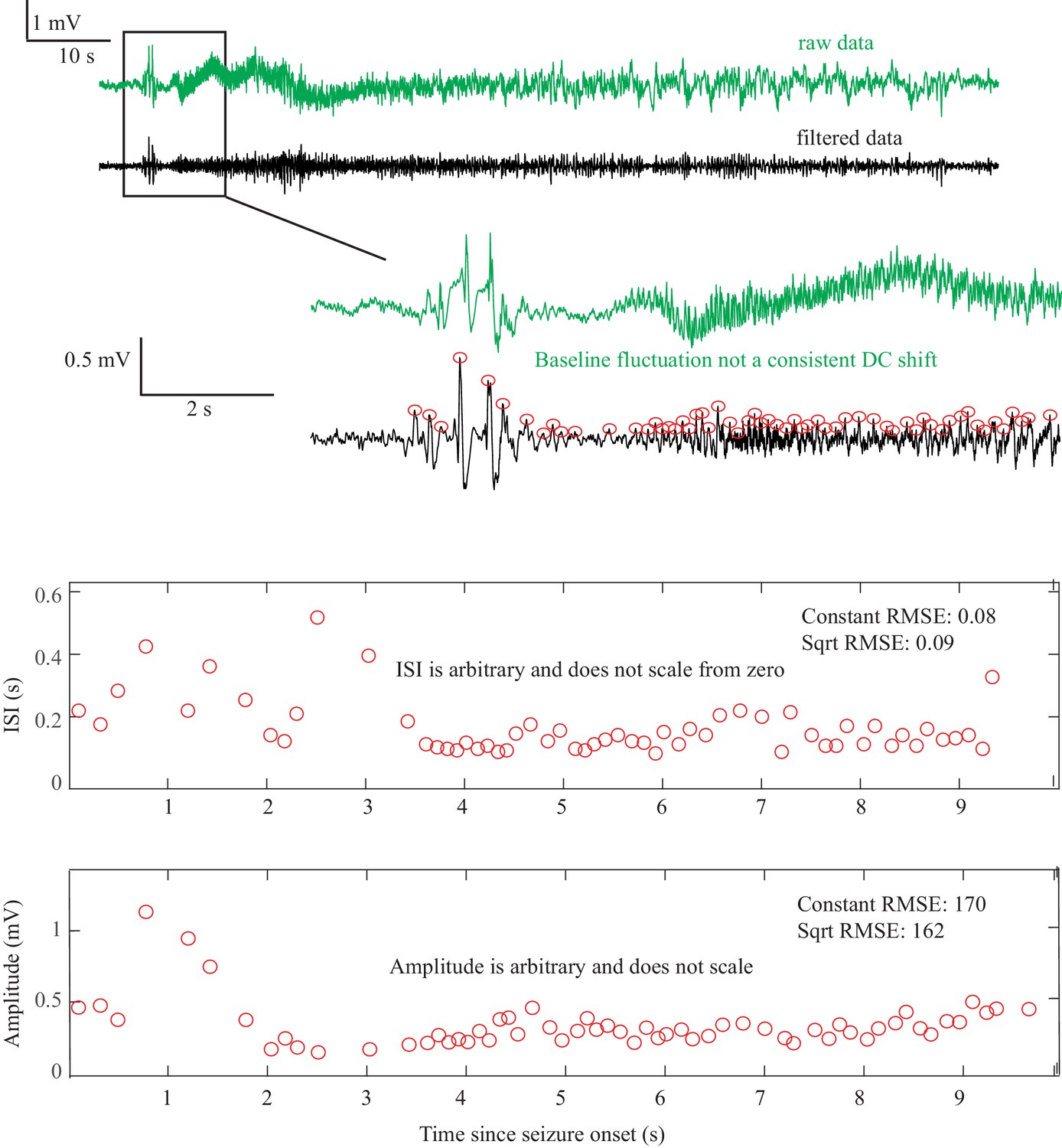
Saddle Node or Subcritical Hopf Onset DC-coupled recordings (green, top) show some baseline fluctuations that are not consistent and too slow to be considered a DC shift.
This recording was capable of showing DC, but this patient’s data did not have a clear DC onset. The ISI and amplitudes are both arbitrary and do not scale from zero. This seizure is consistent with either SN or SubH. Onset Classification: Seizure onset time is somewhat ambiguous, but in this case does not matter for the classification because there is no consistent change regardless of starting point. DC shift: no. Amplitude increasing: no (not consistent). ISI decreasing: no (not consistent). Therefore, this is an arbitrary pattern and is a SN (-DC) or SubH. All reviewers agreed. Offset Classification: Seizure offset is not seen in this view.
Appendix 1—figure 6

SN or SubH onset after delta brush. After a sentinel spike, there is a burst of fast spikes, followed by low-voltage fast spikes that lead into an unusual slow wave similar to the ‘delta brush’ pattern.
The onset pattern is unusual: there are fast polyspikes with arbitrary amplitude after the sentinel spike, then the delta brush, and it is unclear whether there was a DC shift or a slow wave. These early patterns do not fit with any bifurcation. This seizure was labeled as SN or SubH due to the arbitrary amplitude and constant ISI, but is an outlier due to unusual pattern. The delta brush pattern was consistent with Perucca type (vii), see Appendix 1—table 5. Onset Classification: Onset has several unusual patterns in a row. DC shift: no (there appears to be two slow waves at onset, which both begin to recover rather than maintaining a DC shift). Amplitude increasing: no (spikes are quite variable). ISI decreasing: no. Thus, this is an arbitrary pattern and fits with SN (-DC) or SubH. All reviewers agreed. Offset classification: Offset time is somewhat ambiguous, but likely occurs 10 s before the end of the tracing, and is followed by two large polyspike discharges. DC shift: no. Amplitude decreasing: no. ISI increasing: no. This is an arbitrary pattern, so is likely FLC offset. However, this seizure termination is unusual because the offset time is uncertain.
Appendix 1—figure 7
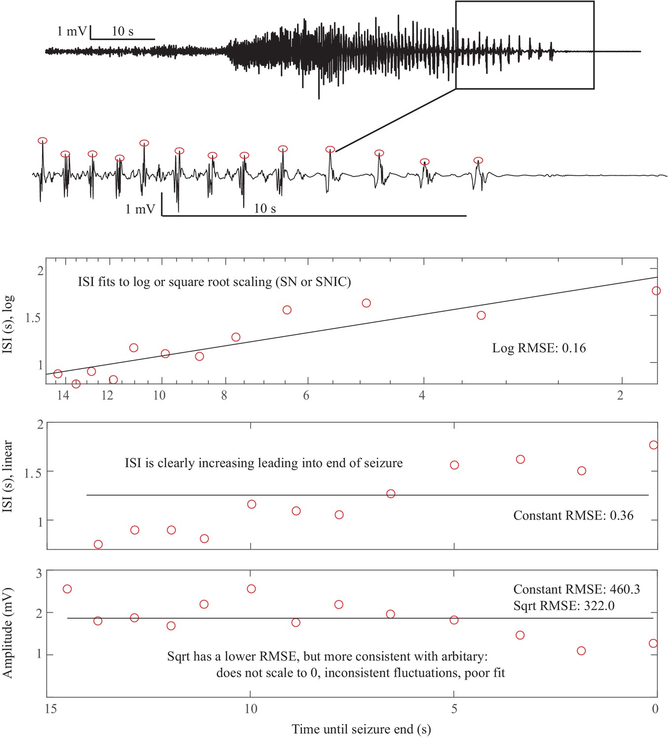
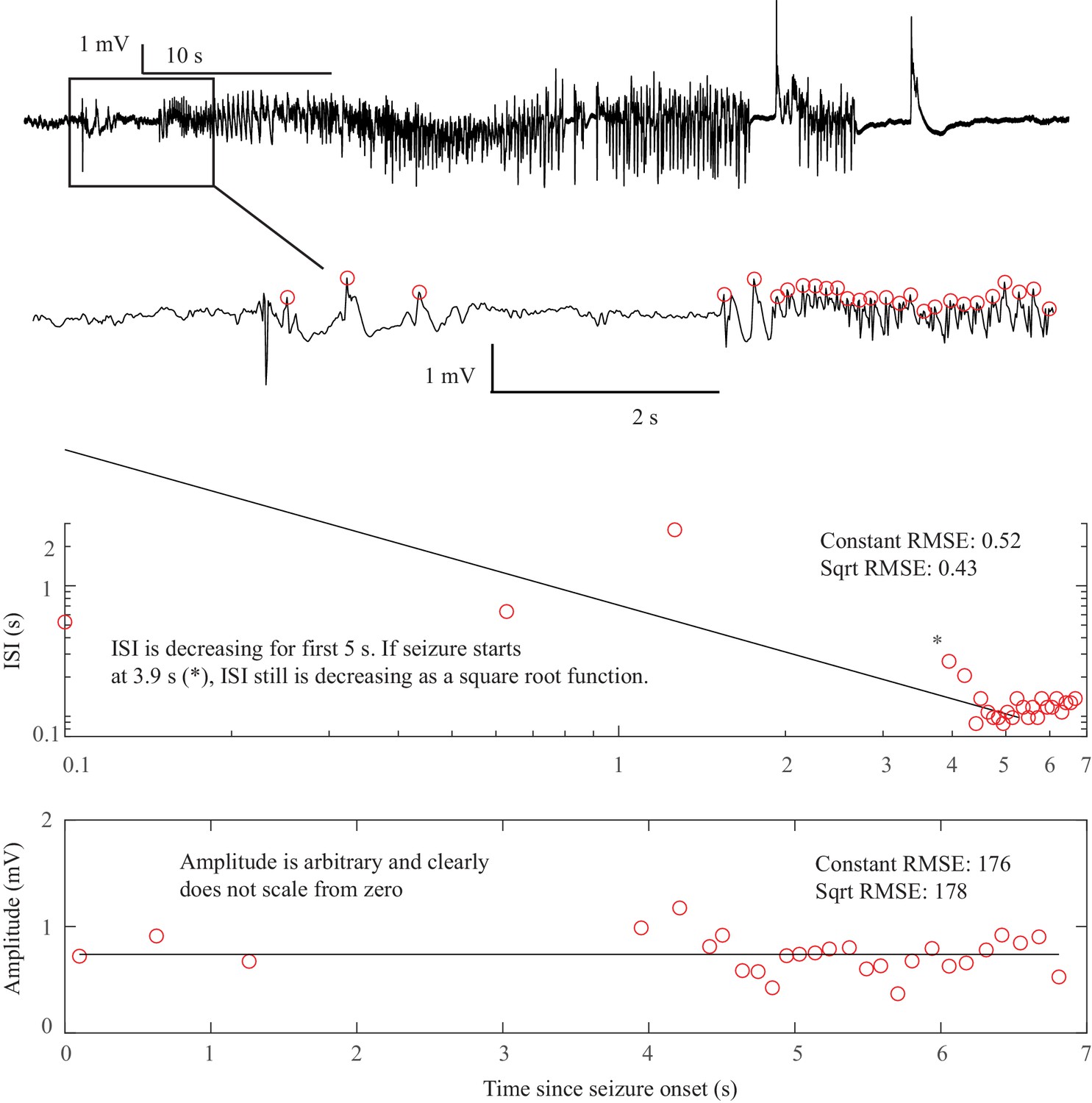
Saddle Homoclinic or SNIC offset. In this case, the terminal ISI clearly increases as the end approaches and the amplitude of spikes does not scale all the way to zero (top).
For visualization, we reverse the spike plots to coincide with the direction of the seizure, but to determine offset t=’time until end of seizure’, that is it is counting down. Hence the ‘0’ is at the right of the plots. ISI shows log scaling in ‘semilogx’ plots, which continues out to 25 s (not shown). The amplitude is somewhat variable but does not diminish to 0. This is consistent with a SH offset. This could also be a SNIC, as a square root function (loglog plot) is very similar at this scale for the ISI (not shown). Offset Classification: DC shift: no. Amplitude decreasing: no. ISI increasing: yes. This is a SH (-DC) or SNIC. This is a very common seizure termination dynamotype. Onset Classification: Difficult to see at this magnification: seizure started with low voltage fast activity near the end of the 10 s scale bar. DC shift: no. Amplitude increasing: no (seizure started about 10 s before the visible increase). ISI decreasing: no. This is a SN (-DC) or SubH.
Appendix 1—figure 8
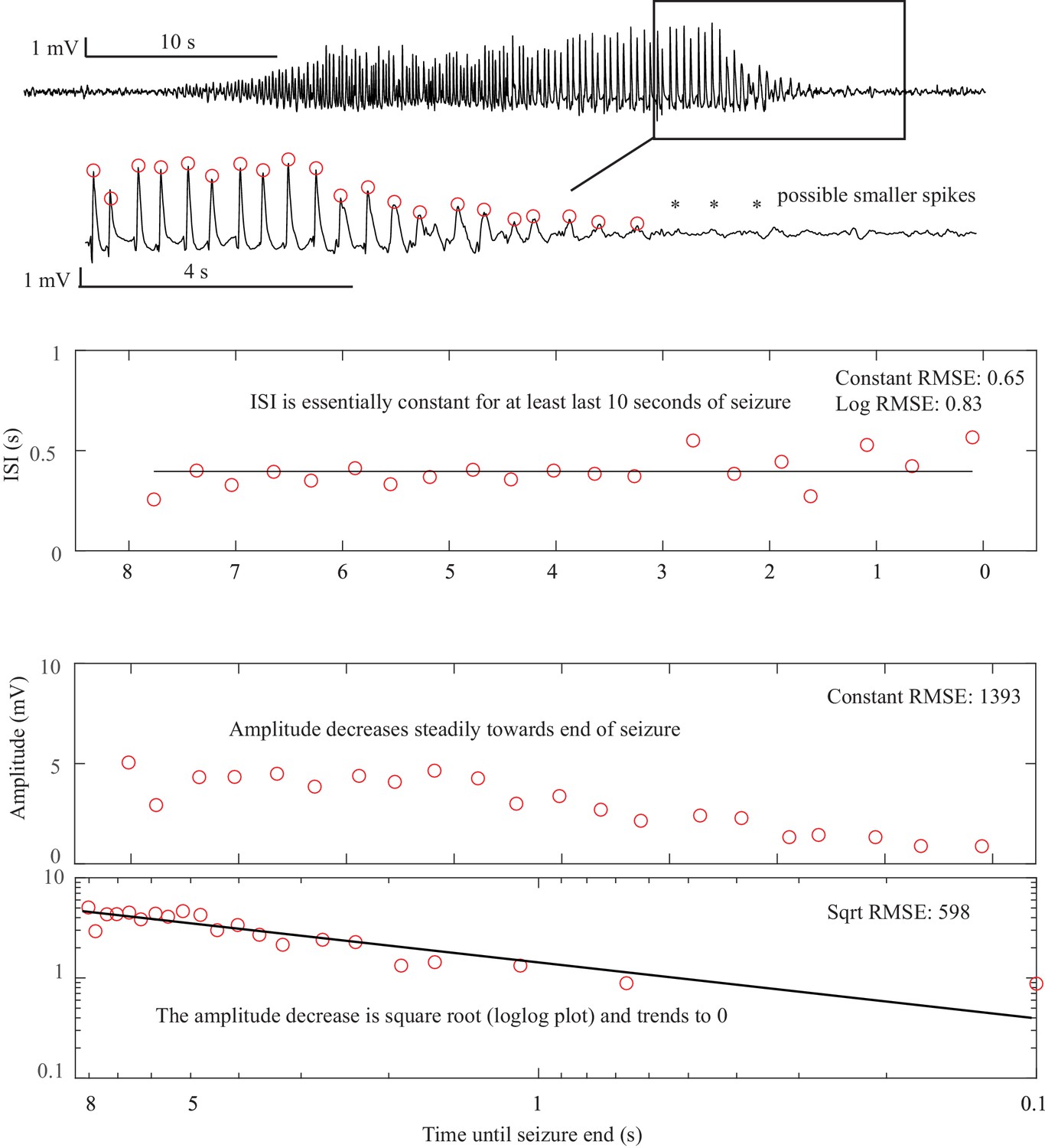
Supercritical Hopf onset and offset. This is the seizure from Figure 2D.
Here, the terminal ISI is nearly constant and does not have any ‘slowing down.’ The amplitude, on the other hand, clearly diminishes and trends to zero as a square root power law by the end of the seizure. There are even some potential smaller spikes seen after the seizure (*), as if the spikes have vanished into the background noise. In this case, the seizure stops because the amplitude, rather than the frequency, has gone to zero. The constant ISI and diminishing amplitude are indicative of the SupH offset. The same pattern occurs at onset. Offset Classification: DC shift: no. Amplitude decreasing: yes. This is a SupH offset. The ISI is also constant, which is consistent but not necessary for the classification due to prioritization. Onset Classification: DC shift: no. Amplitude increasing: yes. This is a SupH onset.
Appendix 1—figure 9
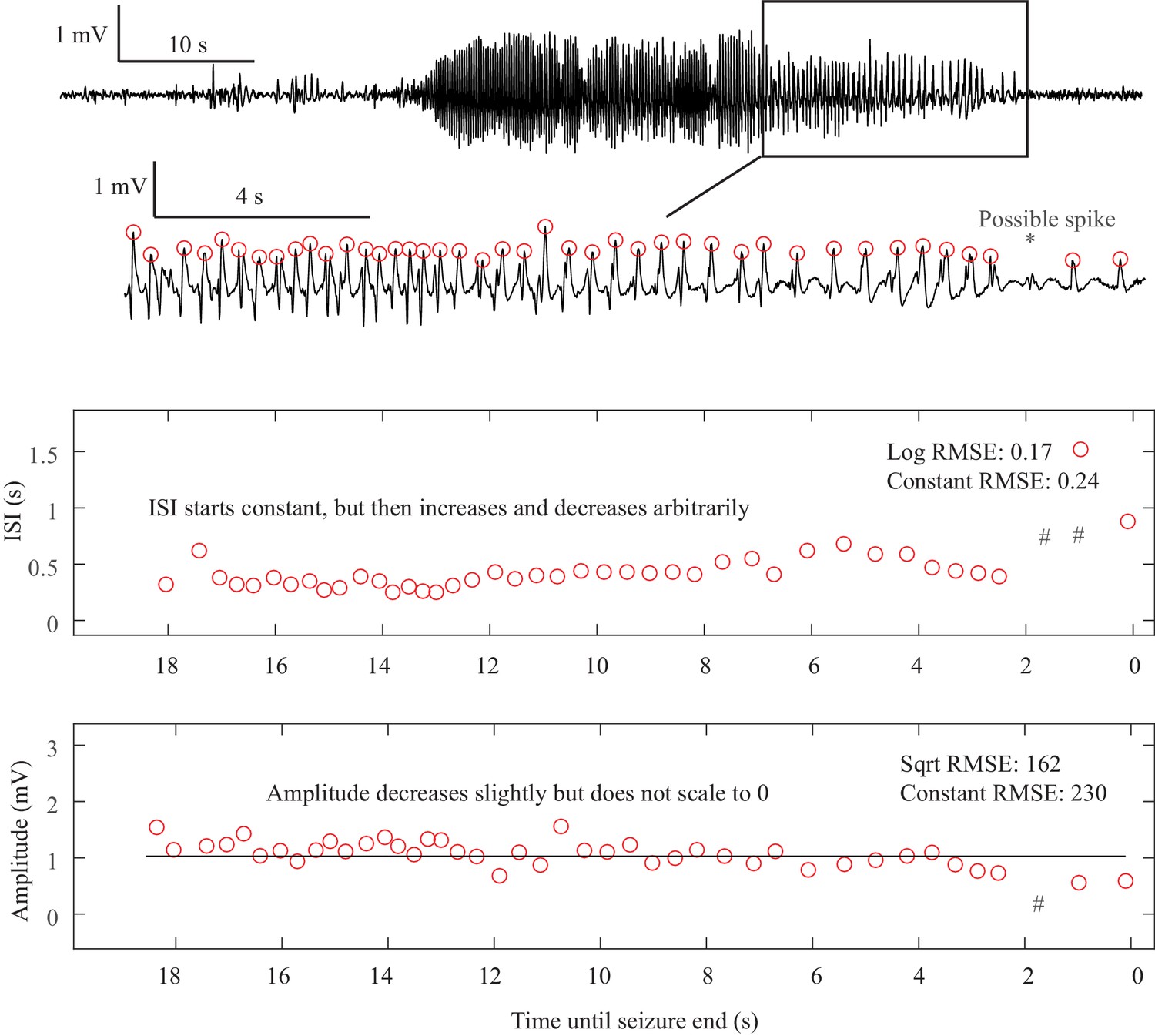
Fold Limit Cycle offset. The primary feature of the FLC is the lack of scaling laws.
In this case, the ISI is constant until 8 s prior to the termination, then begins to increase until 6.5 s, then decreases until 2 s, then increases again. Even if including the one low-amplitude ‘failed’ spike at the *, the ISI is still arbitrary and does not follow log or square root scaling laws (#- location of ISI if the extra spike is included). The end of the seizure is abrupt. This arbitrary pattern is consistent with FLC offset. Other examples of FLC-terminal seizures are shown in Appendix 1—figures 3, 6, 10, 17. Offset Classification: DC shift: no. Amplitude decreasing: no. ISI increasing: no (not consistent). Thus, this is a FLC offset. Onset Classification: No consensus, as it had ambiguous onset time. If it started early it could be a SN(-DC) or SubH, or if it started later it could be a SupH.
Appendix 1—figure 10
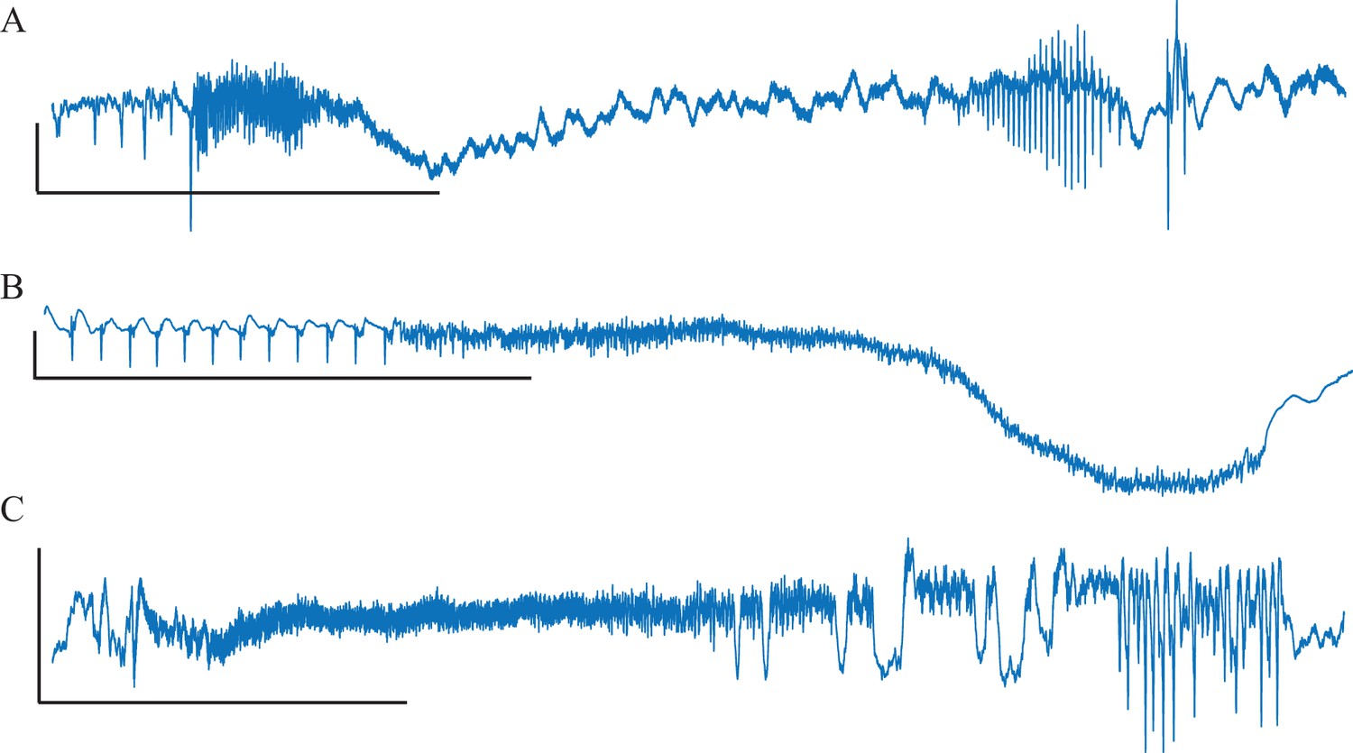
Unusual Fold Limit Cycle seizures.
Each example is a single electrode from a separate patient, showing the voltage trace at the seizure focus. (A) Spike amplitude increases at end of seizure. (B) Abrupt start/stop of low voltage fast activity, without any change in frequency. (Note: the slow downward deflection was too slow to be labeled a DC shift). (C) Seizure with low voltage fast that progresses into arbitrary spike waves. Scale bars: 1 mV by 10 s.
Appendix 1—figure 11
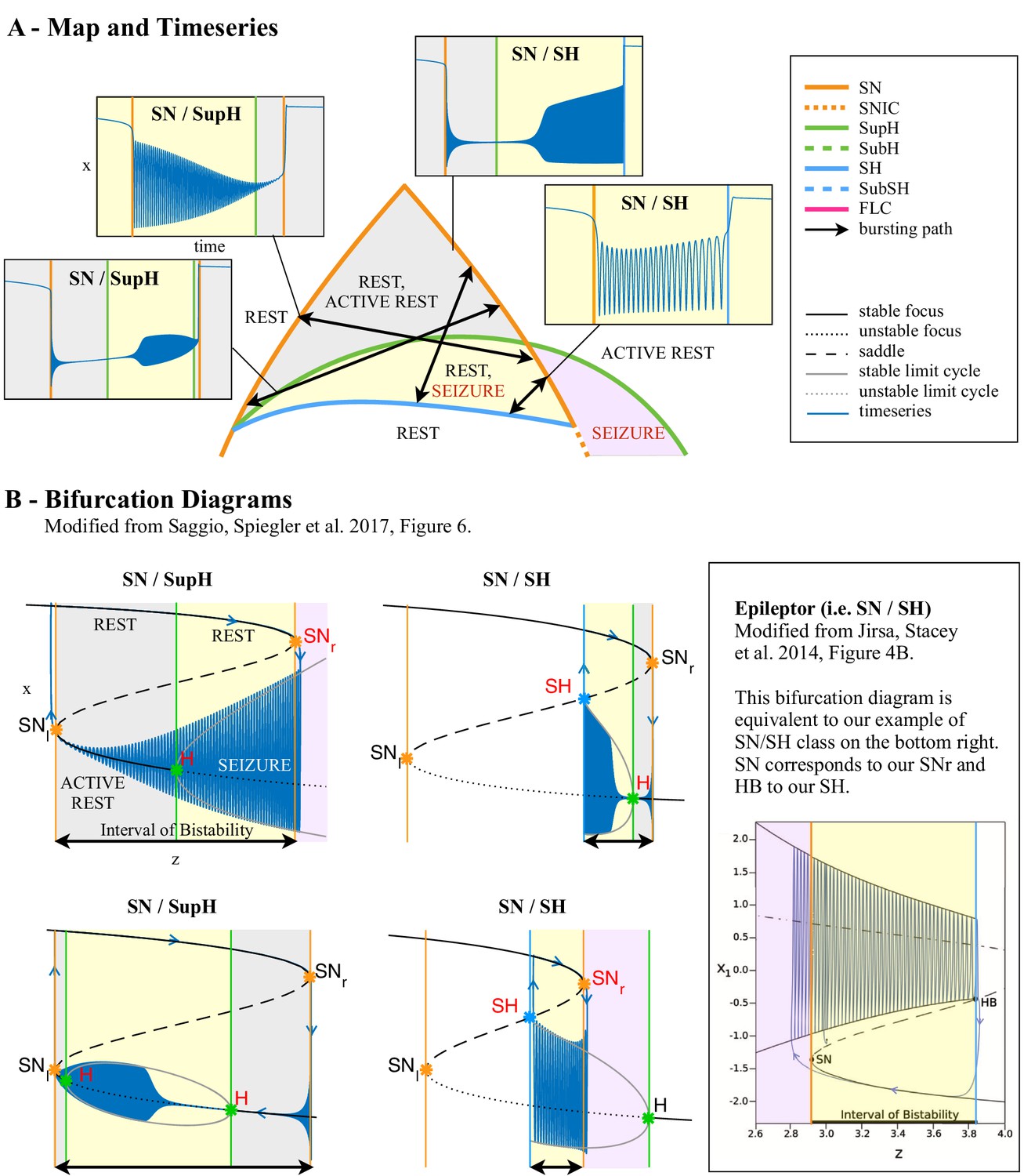
Dynamotypes with baseline shift.
(A) Zoom of the bistability region in the upper part of Figure 4C. In this region, the dynamotypes are combinations of SN, SupH, and SH. All begin with a SN bifurcation, which causes a baseline shift. The background of the timeseries is shaded with the same color of the portion the map traversed. Vertical colored lines mark the value of z at which bifurcations on the map are crossed. Two of the trajectories (top right, bottom left) do not have sustained oscillations until after crossing the SupH bifurcation a short time after the SN onset. (B) Bifurcation diagrams for the same types. Onset and offset bifurcations for the oscillatory phase are marked with red letters. SNr refers to the SN curve on the right of the map, SNl to the SN at the left. Inset: comparison with the ‘Epileptor’ type from Jirsa et al., 2014.
Appendix 1—figure 12
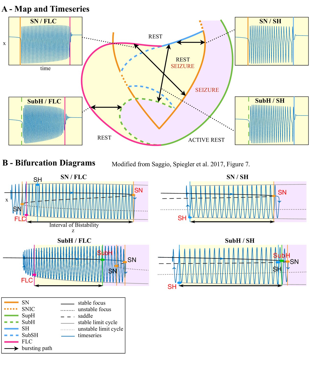
Dynamotypes without baseline shift.
(A) Zoom of the bistability region in the lower part of Figure 4C. For each type possible in this region we show an example of the timeseries. The background of the timeseries is shaded with the same color of the portion the map traversed. Vertical colored lines mark the value of z at which bifurcations on the map are crossed. (B) Bifurcation diagrams for the same types. Onset and offset bifurcations are marked with red letters.
Appendix 1—figure 13
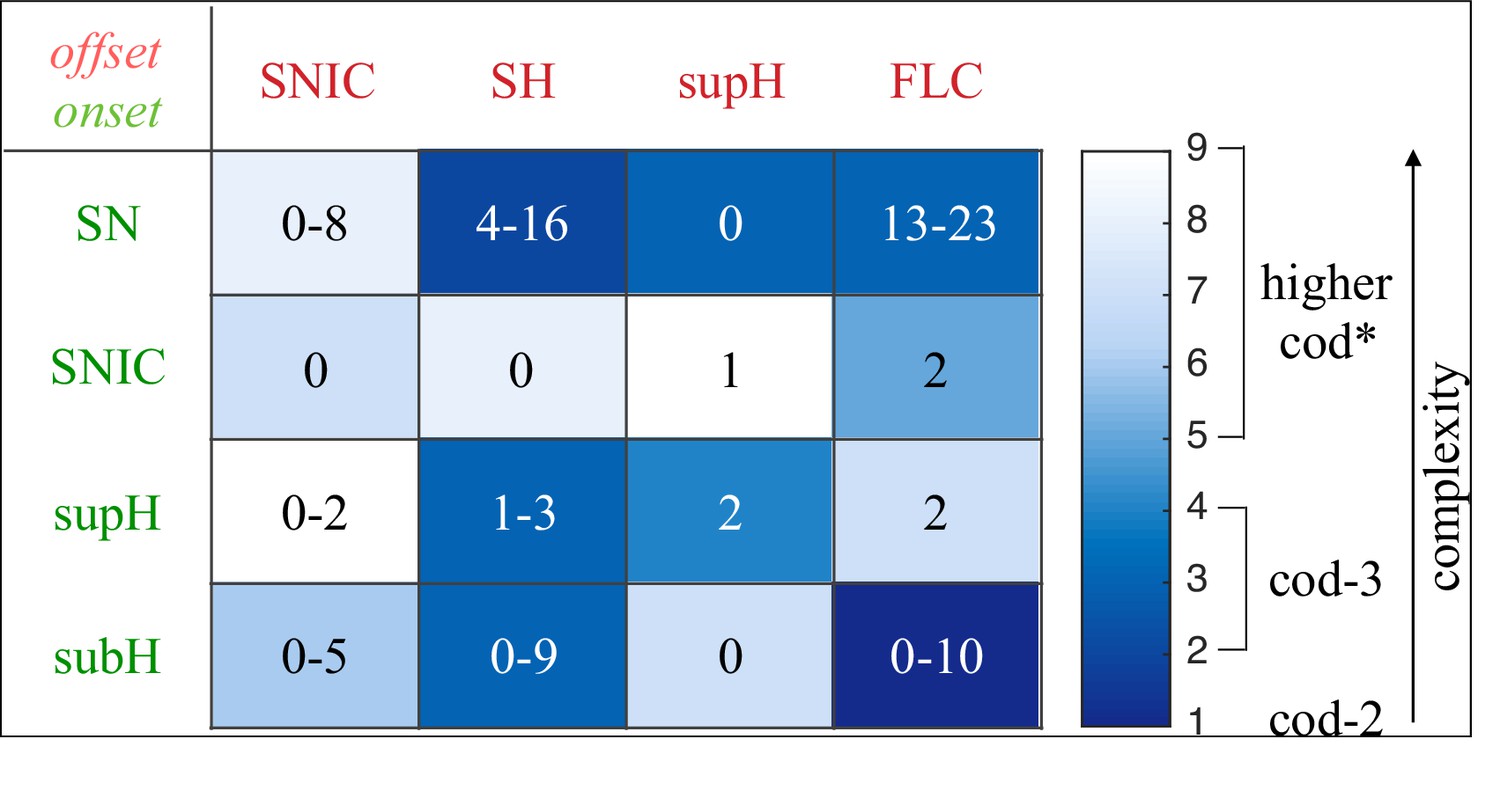
Complexity of types and data classification results.
The complexity of the 16 dynamotypes is shown, with darker colors being the least complex. Superimposed on that are the number of seizures from Figure 2E–F in each type. Note that some of the seizures could not be distinguished between SH and SNIC offsets, or between SN (-DC) and SubH, so for these types there is a range. *-The codimension of some of these types is presumed, see Saggio et al., 2017 for details.
Appendix 1—figure 14

Escape from the bistability region into the seizure-only region.
(A) In some of the simulations performed with an ultra-slow downward drift and noise, the system escaped from the bistability region (yellow) into the seizure-only region (lavender). The escape could occur directly through SN (orange curve), as in Simulation 1, or passing below SH (blue curve) and then through SN, as in Simulation 2. (B-C) Time series for Simulation 1 and 2. The clinical relevance of this is to illustrate how some episodes of status epilepticus might arise uniformly (B) while others have a stuttering onset (C).
Appendix 1—figure 15
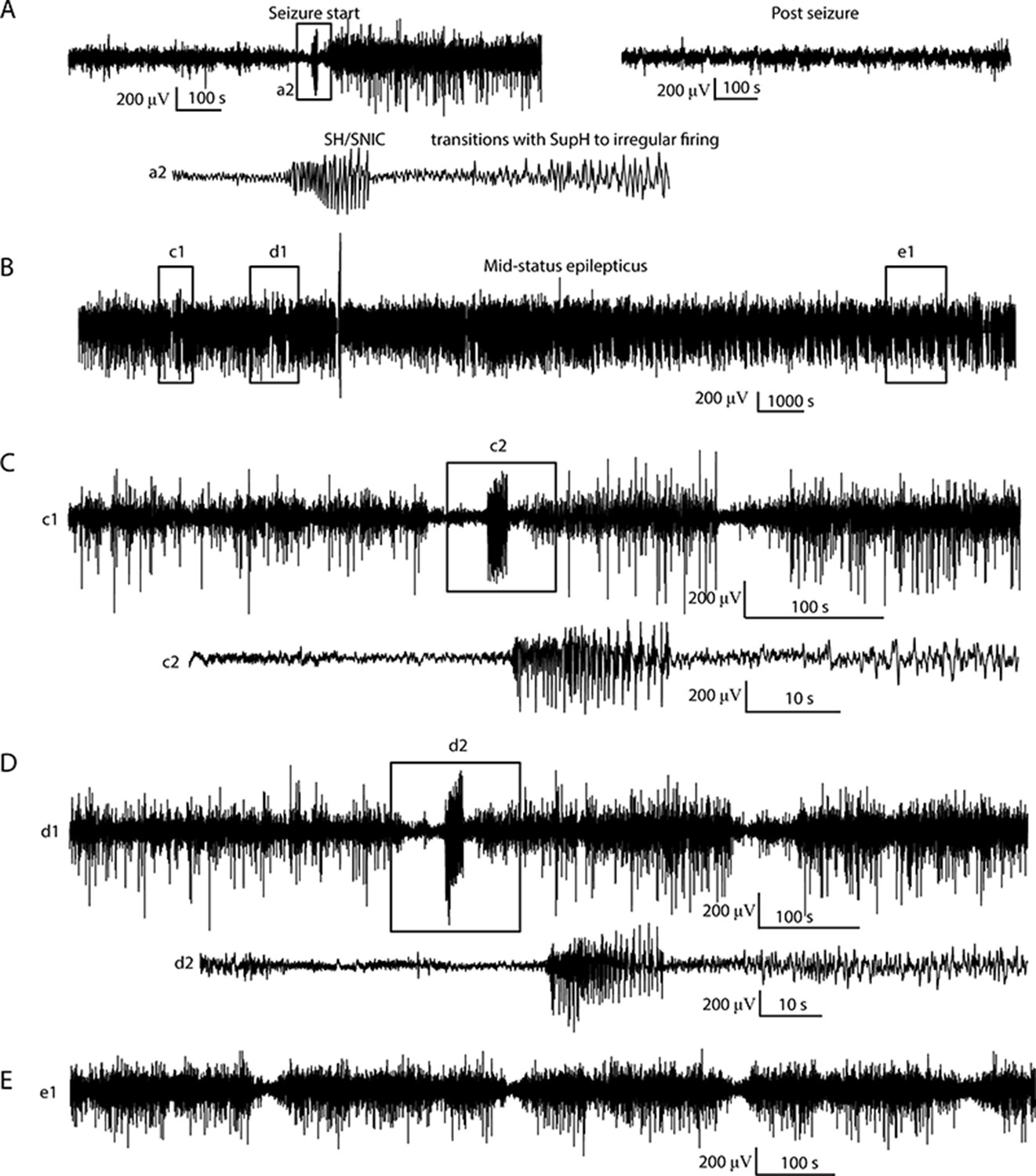
Status Epilepticus patient 1.
(A) Initiation (left) of seizure that begins to terminate with a SH/SNIC bifurcation, then transitions into a SupH onset. The post-seizure baseline (right) returns to prior levels. The seizure lasted >24 hr, but due to signal dropout the exact time of termination was not recorded. Inset a2: expanded view of indicated portion of seizure start. (B) Subclinical status epilepticus was characterized by irregular firing interspersed with periods of organized, lower amplitude EEG. (C, D) Expanded view of (c1, d1) from B, with further expansion of (c2, d2). The irregular firing organizes several times into discrete seizures that nearly terminate with SH dynamics, but revert to the previous pattern. (E) Later in the seizure, there is waxing/waning of the firing pattern, similar to Figure 5D–F.
Appendix 1—figure 16

Status Epilepticus patient 2.
(A) Onset and offset of a seizure lasting 5 hr were both SupH bifurcations. (B) During the seizure, there were many transitions in which the dynamics altered. Top: voltage trace. Bottom: interspike intervals (ISI) show multiple periods in which nearly-constant ISI is interrupted by disorganized firing. Blue lines indicate these transition periods. (C) Expanded view of red box in B. (D) Expanded view of green box in C. Green circles indicate runs of highly periodic, 7 Hz spike waves, which became more frequent later in seizure.
Appendix 1—figure 17
Seizure with acceleration of spike frequency at seizure terminus In this case, the ISI progressively decreases and follows a reverse power law.
The amplitude is arbitrary. This seizure was labeled as a FLC bifurcation for taxonomical purposes as it did not fit with any other single bifurcation.
Appendix 1—figure 18
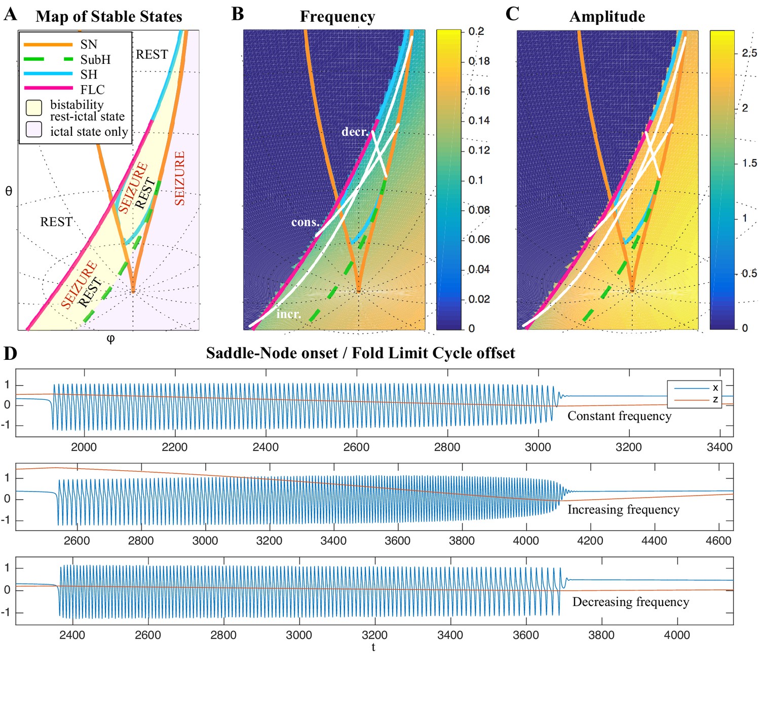
Varied frequency behavior of FLC offsets.
Depending on how close the trajectory comes to the SH offset, an FLC offset can have a wide range of frequency behaviors. We show examples for three frequency trends for the FLC bifurcation. (A) Portion of the map in which the SubH/FLC type can be found. (B-C) Frequency and amplitude trajectories of three different seizures showing constant, increasing, and decreasing frequency. (D) Simulations for the paths shown in B-C. Note the last few spikes drop in amplitude precipitously, characteristic of the FLC releasing from the limit cycle (which has a finite amplitude when it disappears) and settling on the fixed point. This is different from the square-root decreasing amplitude of the SupH bifurcation, which is instead caused by a slow decrease in the amplitude of the limit cycle itself, in this latter case the limit cycle disappears when zero amplitude is reached.
Appendix 1—figure 19
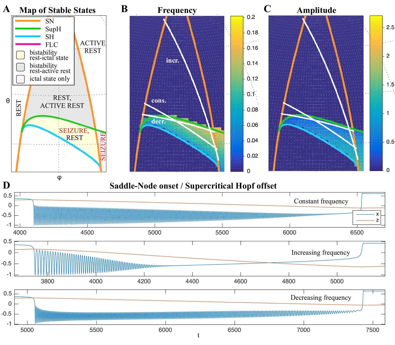
Frequency behavior of SupH offsets.
The trajectory of seizure offset in SupH is influenced by the SH curve, allowing for constant, increasing and decreasing frequency trends. (A) Portion of the map in which the SN/SupH type can be found. (B-C) Frequency and amplitude trajectories of three different seizures showing constant, increasing, and decreasing frequency. (D) Simulations for the paths shown in B-C. Note the amplitude in each case is very characteristic of the SupH, despite the different frequency behavior.
Author response image 1
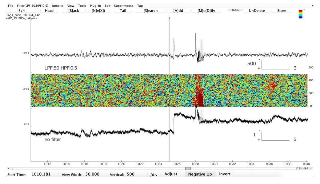
Representative example of an epileptiform discharge recorded in the hippocampus in a freely moving animal (Tetanus Toxin injected in the hippocampus to create a focus).
The upper trace is in AC, the lower one is in DC. Note that the first AC “spike”, which would be qualified as “isolated interictal spike” is actually a very large DC shift. The second “spike” is part of an epileptic discharge. Note that AC filtering artificially shortens the true duration of the event. The large DC shift will eventually recover (not shown).
Tables
Appendix 1—table 1
Visual classification system.
Classification relies upon visualization of the given features. In case of multiple features present, the bifurcation listed on top takes priority. DC shift: a sharp deflection >5 times the background that occurs in <0.5 s, then lasts >1 s. Constant: the value is consistent and does not trend upward or downward for 10 spikes. Arbitrary: no consistent unimodal trend over 10 spikes.
| Onset | |
|---|---|
| DC Shift | SN(+DC) |
| Amplitude increasing | SupH |
| Interspike interval (ISI) decreasing (i.e. frequency increasing) | SNIC |
| ISI and Amplitude constant/arbitrary (no DC shift) | SN(-DC) or SubH |
| Offset | |
| DC Shift | SH(+DC) |
| Amplitude decreasing | SupH |
| ISI increasing (frequency decreasing) (no DC shift) | SH(-DC) or SNIC |
| ISI and amplitude constant/arbitrary (no DC shift) | FLC |
Appendix 1—table 2
Reviewer agreement on simulated data.
Reviewers were highly consistent with each other in the simulated data. The interrater reliability is extremely high, as the p-value (Fleiss Kappa, three reviewers) is negligible.
| Unanimous | 2/3 agree | No consensus | P value | |
|---|---|---|---|---|
| Onset (N = 240) | 192 | 44 | 4 | p<4.9 e-324 |
| Offset (N = 240) | 189 | 51 | 0 | p<4.9 e-324 |
Appendix 1—table 3
Accuracy identifying bifurcations in clinical data.
A. Reviewers were highly consistent with each other scoring the bifurcations in the clinical data. (Fleiss Kappa, three reviewers). Each patient was stratified based upon whether their EEG had DC-coupled recordings, as the non-DC group could not disambiguate SN or SH with DC shifts. B. The model fit of the automated features to each chosen bifurcation was performed versus human majority vote, then bootstrapped as in Step 1. The chosen model parameters were clearly highly descriptive of chosen bifurcations in DC onset and offset and non-DC offset. As expected, the lack of DC coupling makes it difficult to disambiguate the four onset bifurcations.
| A.Reviewer agreement on human data | ||
|---|---|---|
| Dc (N = 51) | Non-DC (N = 69) | |
| Onset | p=1.78e-15 | p=4.51e-12 |
| Offset | p=4.51e-11 | p=9.72e-4 |
| B. Automated features permutation test | ||
| DC | Non-DC | |
| Onset | p<1e-4 | p=0.0969 |
| Offset | p=7e-4 | p<1e-4 |
Appendix 1—table 4
Comparison of bifurcations with metadata.
All available patient metadata from all centers are included. CD: cortical dysplasia (including two heterotopias). MTS: mesial temporal sclerosis. T: tumor. O: other. F: frontal. Oc: Occipital. P: parietal. Te: temporal.
| Onset | Sex | Age | Pathology | Location | |||||||||
|---|---|---|---|---|---|---|---|---|---|---|---|---|---|
| M | F | 1–20 | 21–40 | 41–60 | CD | MTS | T | O | Te | F | Oc | P | |
| SN-SubH | 30 | 23 | 13 | 29 | 10 | 20 | 17 | 1 | 1 | 26 | 12 | 5 | 8 |
| SNIC | 3 | 3 | 4 | 2 | 0 | 2 | 2 | 1 | 1 | 2 | 0 | 0 | 0 |
| SupH | 10 | 4 | 2 | 3 | 9 | 2 | 5 | 2 | 0 | 9 | 4 | 2 | 2 |
| Offset | |||||||||||||
| SH-SNIC | 17 | 13 | 5 | 16 | 8 | 10 | 10 | 1 | 1 | 17 | 9 | 2 | 3 |
| SupH | 1 | 0 | 0 | 0 | 1 | 0 | 1 | 0 | 0 | 1 | 1 | 0 | 0 |
| FLC | 23 | 19 | 12 | 19 | 9 | 14 | 12 | 3 | 1 | 20 | 8 | 5 | 8 |
Appendix 1—table 5
Comparison of visual with dynamic classifications.
Top: Metadata stratified by Perucca classification. There is no clear correlation between Perucca onset type and any of the clinical metadata. Bottom: Comparison of Perucca visual onset classification with our bifurcation analysis. There was no significant correlation between the two classifications. Note that numbers sometimes do not reconcile between different sections and between Appendix 1—table 4 and 5due to lack of metadata in some patients. U: unclassifiable.
| Onset | Sex | Age | Pathology | Location | |||||||||
|---|---|---|---|---|---|---|---|---|---|---|---|---|---|
| M | F | 1–10 | 21–40 | 41–60 | CD | MTS | T | O | Te | F | Oc | P | |
| i. | 15 | 15 | 7 | 10 | 12 | 9 | 10 | 1 | 1 | 18 | 5 | 1 | 5 |
| ii. | 9 | 8 | 5 | 8 | 4 | 6 | 6 | 2 | 0 | 7 | 5 | 4 | 3 |
| iii. | 13 | 10 | 6 | 14 | 3 | 7 | 8 | 0 | 1 | 13 | 7 | 0 | 4 |
| iv. | 3 | 2 | 2 | 3 | 0 | 2 | 2 | 0 | 0 | 3 | 1 | 0 | 1 |
| v. | 2 | 2 | 2 | 2 | 0 | 1 | 0 | 0 | 1 | 0 | 1 | 2 | 1 |
| vii. | 1 | 1 | 0 | 2 | 0 | 0 | 0 | 0 | 0 | 0 | 1 | 0 | 0 |
| U | 5 | 2 | 1 | 5 | 1 | 1 | 2 | 2 | 1 | 6 | 4 | 0 | 0 |
| Jirsa onset | Jirsa offset | ||||||||||||
| SN/SubH | SNIC | SupH | Sh/SNIC | SupH | FLC | ||||||||
| Perucca Onset | i. | 21 | 2 | 8 | 12 | 0 | 17 | ||||||
| ii. | 14 | 2 | 6 | 10 | 0 | 13 | |||||||
| iii. | 22 | 1 | 4 | 12 | 1 | 14 | |||||||
| iv. | 4 | 1 | 0 | 3 | 0 | 3 | |||||||
| v. | 3 | 0 | 2 | 1 | 1 | 3 | |||||||
| vii. | 2 | 0 | 0 | 0 | 0 | 2 | |||||||
| U | 1 | 0 | 2 | 2 | 0 | 0 | |||||||
| Jirsa Offset | SH/SNIC | 30 | 3 | 14 | |||||||||
| SupH | 1 | 1 | 3 | ||||||||||
| FLC | 53 | 3 | 7 | ||||||||||
Additional files
Download links
A two-part list of links to download the article, or parts of the article, in various formats.
Downloads (link to download the article as PDF)
Open citations (links to open the citations from this article in various online reference manager services)
Cite this article (links to download the citations from this article in formats compatible with various reference manager tools)
A taxonomy of seizure dynamotypes
eLife 9:e55632.
https://doi.org/10.7554/eLife.55632


