The development of active binocular vision under normal and alternate rearing conditions
- Frankfurt Institute for Advanced Studies (FIAS), Germany
- Department of Ophthalmology, Child Vision Research Unit, Goethe University, Germany
- Department of Electronic and Computer Engineering, Hong Kong University of Science and Technology, China
Figures
Figure 1
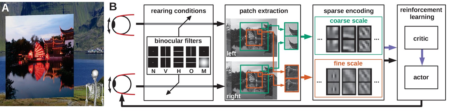
Model overview.
(A) The agent looks at the object plane in the simulated environment. (B) Architecture of the model. Input images are filtered to simulate alternate rearing conditions (N: normal, V: vertical, H: horizontal, O: orthogonal, M: monocular). Binocular patches are extracted at a coarse and a fine scale (turquoise and orange boxes) with different resolutions. These patches are encoded via sparse coding and combined with the muscle activations to form a state vector for actor critic reinforcement learning. The reconstruction error of sparse coding indicates coding efficiency and serves as a reward signal (purple arrow) to train the critic. The actor generates changes in muscle activations, which result in differential rotations of the eyeballs and a new iteration of the perception-action cycle.
Figure 2 with 1 supplement
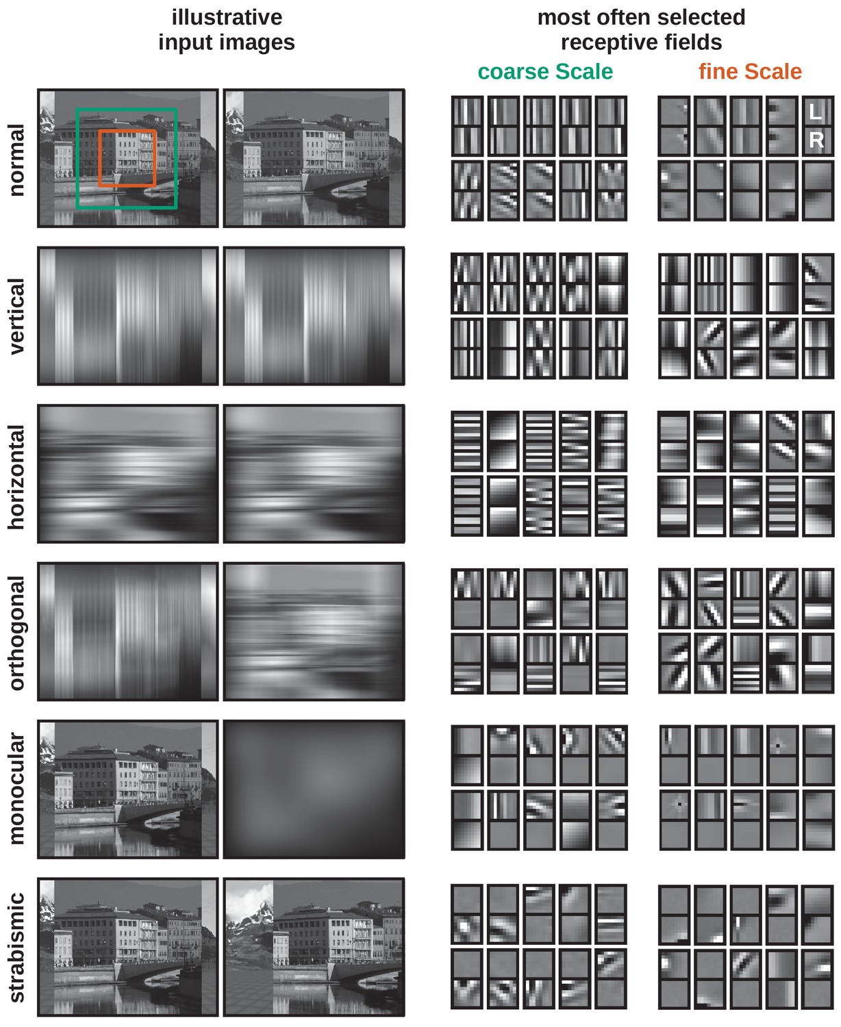
Visual input and learned receptive fields under different rearing conditions.
Left: Illustration of visual inputs under the different rearing conditions. Except for the normal condition, the images are convolved with different Gaussian filters to blur out certain orientations or simulate monocular deprivation. To simulate strabismus the right eye is rotated inward by 10°, so that neurons receive non-corresponding inputs to their left and right eye receptive fields. The structures behind the object plane depict a background image in the simulator. Right: Examples of binocular RFs for the fine and coarse scale learned under the different rearing conditions after 0.5 million iterations. For each RF, the left eye and right eye patches are aligned vertically. In each case, the 10 RFs most frequently selected by the sparse coding algorithm are shown.
-
Figure 2—source data 1
Coarse and fine scale RFs in vectorized form for all rearing conditions.
- https://cdn.elifesciences.org/articles/56212/elife-56212-fig2-data1-v2.zip
Figure 2—figure supplement 1
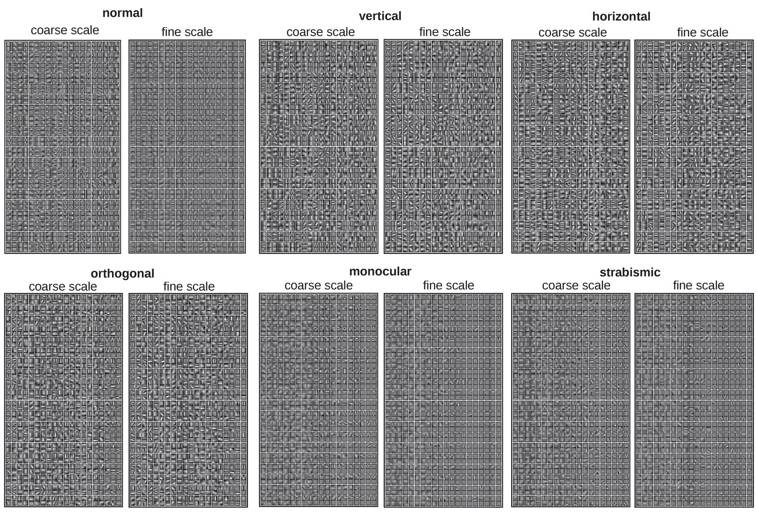
All learned RFs for the six rearing conditions.
Complete set of all RFs that are learned during training for all different rearing conditions. .
Figure 3
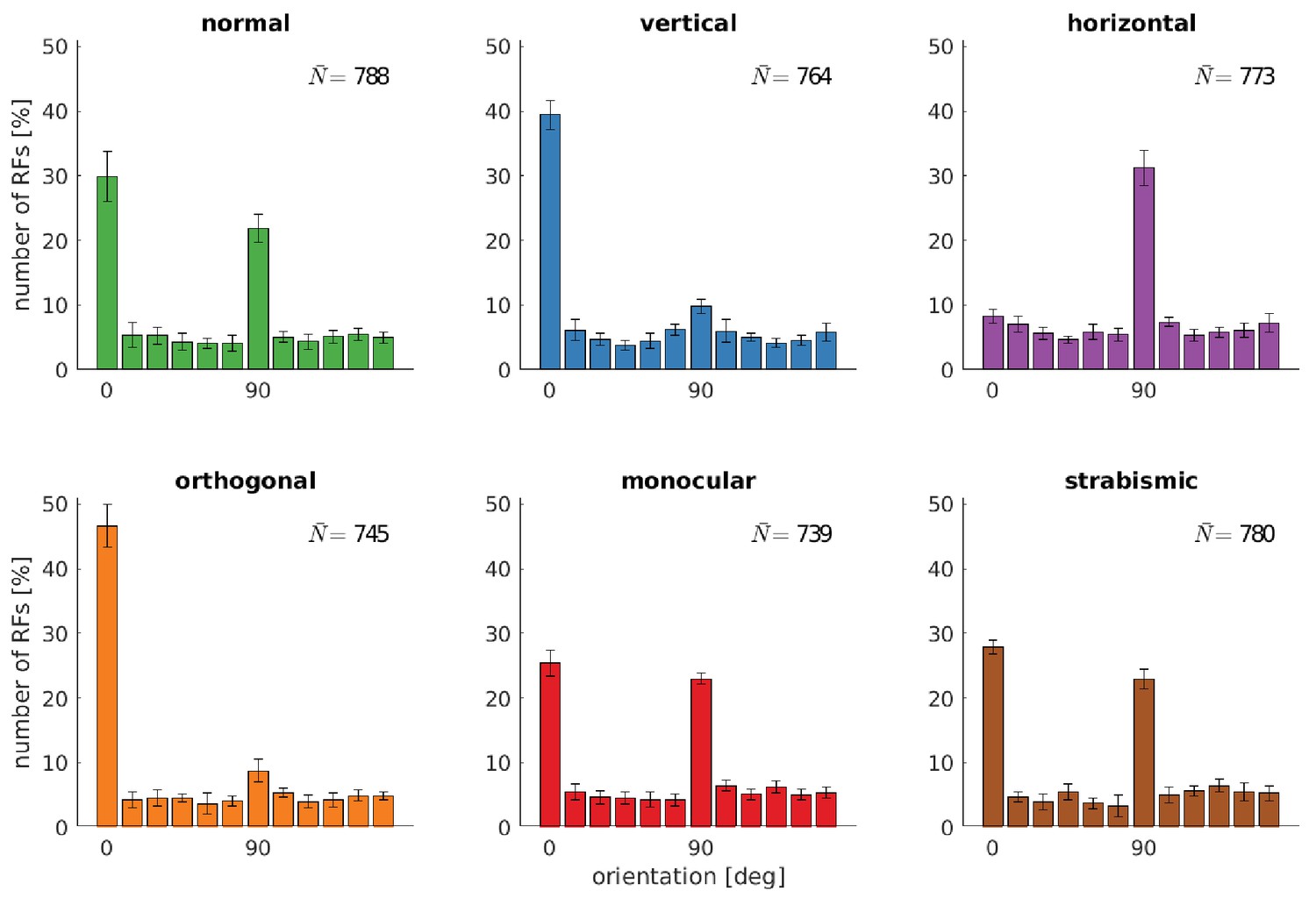
Distributions of RFs' orientation preference for different rearing conditions.
Displayed are the preferred orientations resulting from fitting Gabor wavelets to the learned RFs of the left eye. Coarse and fine scale RFs have been combined (800 in total). The error bars indicate the standard deviation over five different simulations. describes the average number of RFs that passed the selection criterion for the quality of Gabor fitting (see Materials and methods).
-
Figure 3—source data 1
Orientation tuning for all rearing conditions.
- https://cdn.elifesciences.org/articles/56212/elife-56212-fig3-data1-v2.zip
Figure 4
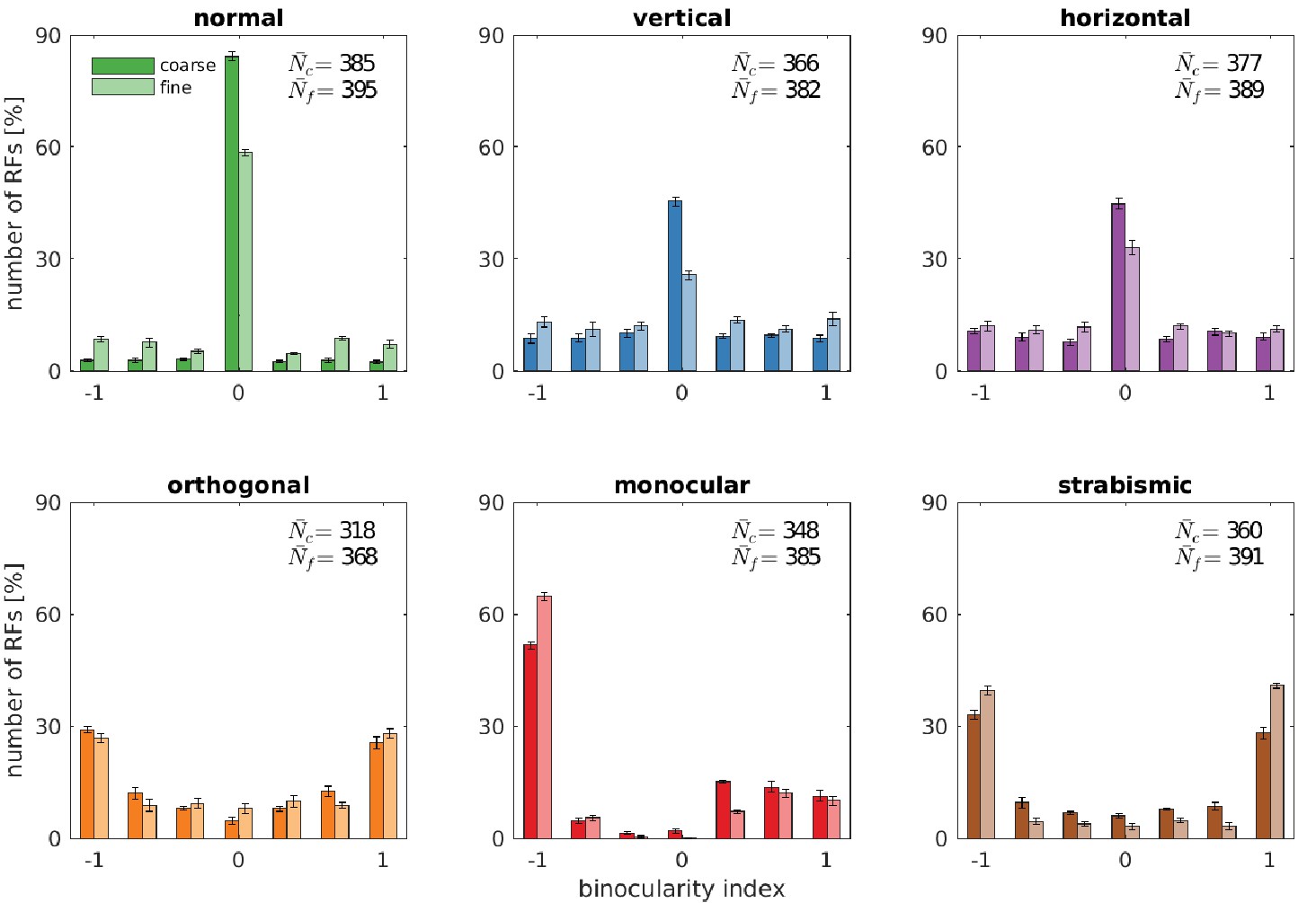
Binocularity distributions for different rearing conditions.
The binocularity index ranges from −1 (monocular left) over 0 (binocular) to 1 (monocular right). Error bars indicate the standard deviation over five different simulations. and are the average number of basis functions (out of a total of 400) that pass the selection criterion for Gabor fitting (see Materials and methods).
-
Figure 4—source data 1
Binocularity values for all rearing conditions for coarse and fine scale.
- https://cdn.elifesciences.org/articles/56212/elife-56212-fig4-data1-v2.zip
Figure 5 with 2 supplements
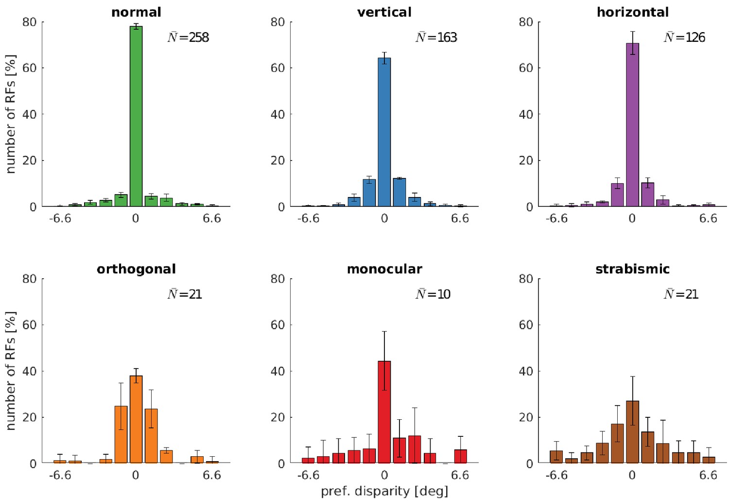
Distributions of neurons’ preferred disparities for different rearing conditions.
The neurons’ preferred disparities are extracted from the binocular Gabor fits. Presented are the averaged data for the coarse scale from five simulations. describes the average number of neurons meeting the selection criteria (see Materials and methods).
-
Figure 5—source data 1
Coarse scale disparity tuning for all rearing conditions.
- https://cdn.elifesciences.org/articles/56212/elife-56212-fig5-data1-v2.zip
-
Figure 5—source data 2
Fine scale disparity tuning for all rearing conditions. .
- https://cdn.elifesciences.org/articles/56212/elife-56212-fig5-data2-v2.zip
-
Figure 5—source data 3
Coarse scale disparity tuning for training with a constant angle of 3°.
- https://cdn.elifesciences.org/articles/56212/elife-56212-fig5-data3-v2.zip
Figure 5—figure supplement 1
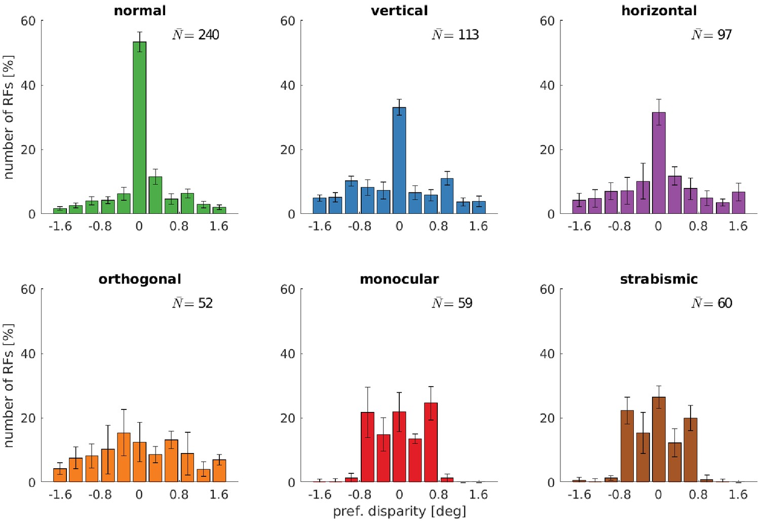
Disparity tuning for the fine scale.
Disparity tuning of the fine scale of models that were trained under different rearing conditions.
Figure 5—figure supplement 2
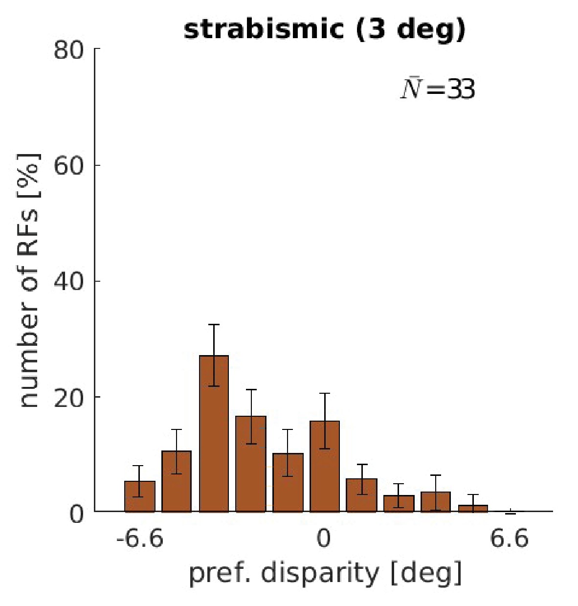
Disparity tuning for training with a constant strabismic angle of 3°.
Disparity tuning of a model that was trained with a constant strabismic angle of 3°. Note the marked similarity to Figure 2 in Shlaer, 1971. Depicted are the results from the coarse scale only.
Figure 6
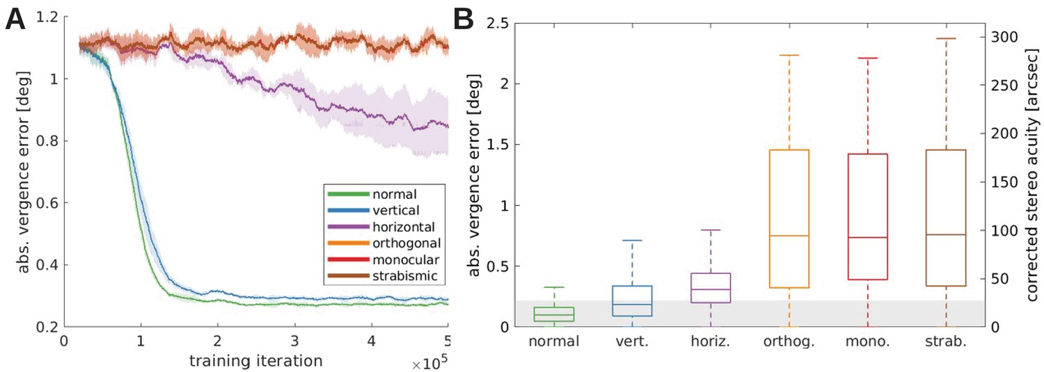
Vergence performance of models trained under different rearing conditions.
(A) Moving average of the vergence error during training. The vergence error is defined as the absolute difference between the actual vergence angle and the vergence angle required to correctly fixate the object. Shaded areas indicate the standard deviation over five different simulations. The curves for orthogonal, monocular, and strabismic conditions are overlapping, see text for details. (B) Vergence errors at the end of training after correction of any visual aberrations. Shown is the distribution of vergence errors at the end of a fixation (20 iterations) for previously unseen stimuli. Outliers have been removed. The gray shaded area indicates vergence errors below 0.22°, which corresponds to the model’s resolution limit. The second y-axis shows values corrected to match human resolution (see Materials and methods for details).
-
Figure 6—source data 1
Training performance for all rearing conditions recorded every 10 iterations.
- https://cdn.elifesciences.org/articles/56212/elife-56212-fig6-data1-v2.zip
-
Figure 6—source data 2
Performance at testing for all rearing conditions.
- https://cdn.elifesciences.org/articles/56212/elife-56212-fig6-data2-v2.zip
Figure 7
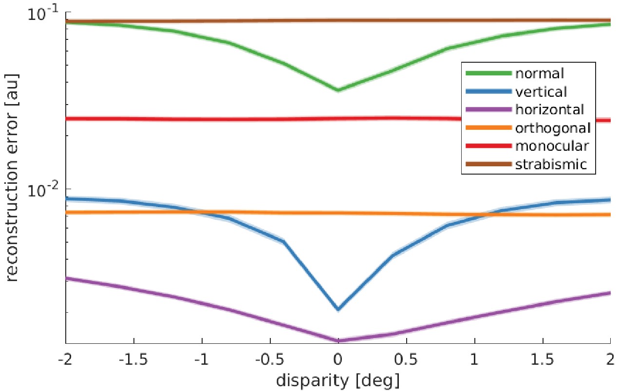
Reward landscape at the end of training for the different rearing conditions.
Shown is the logarithm of the sparse coder’s reconstruction error as a function of disparity. The negative reconstruction error is used as the reward for learning vergence movements. Data are averaged over 10 stimuli not encountered during training, three different object distances (0.5, 3, and 6 m), and five simulations for every condition. The shaded area represents one standard error over the five simulations. Only those models that receive corresponding input to left and right eye display a reconstruction error that is minimal at zero disparity. These are the only models that learn to verge the eyes.
-
Figure 7—source data 1
Rewards for 5 random seeds, 3 object distances, 11 different disparity values, 10 different input images and 2 scales for all six rearing conditions.
- https://cdn.elifesciences.org/articles/56212/elife-56212-fig7-data1-v2.zip
Figure 8 with 2 supplements

The effect of unequal image size (aniseikonia) on the development of binocular vision.
(A) Vergence error as a function of time for different degrees of aniseikonia. (B) Number of RFs tuned to vertical disparities for different degrees of aniseikonia during learning. (C) Stereo acuity when different degrees of aniseikonia are introduced after normal rearing. The solid line depicts a quadratic fit to the data. The corrected stereo acuity on the right y-axis corrects for the lower visual resolution of the model compared to humans.
-
Figure 8—source data 1
Vergence error over training time measured every 10 iterations for all degrees of aniseikonia (five random seeds). .
- https://cdn.elifesciences.org/articles/56212/elife-56212-fig8-data1-v2.zip
-
Figure 8—source data 2
Tuning to vertical disparities for all degrees of aniseikonia (five random seeds).
- https://cdn.elifesciences.org/articles/56212/elife-56212-fig8-data2-v2.zip
-
Figure 8—source data 3
Vergence performance of normal models tested under different degrees of aniseikonia (five random seeds).
- https://cdn.elifesciences.org/articles/56212/elife-56212-fig8-data3-v2.zip
-
Figure 8—source data 4
Binocularity values for all degrees of aniseikonia.
- https://cdn.elifesciences.org/articles/56212/elife-56212-fig8-data4-v2.zip
-
Figure 8—source data 5
Orientation tuning for all degrees of aniseikonia.
- https://cdn.elifesciences.org/articles/56212/elife-56212-fig8-data5-v2.zip
-
Figure 8—source data 6
Alls RFs for all degrees of aniseikonia.
- https://cdn.elifesciences.org/articles/56212/elife-56212-fig8-data6-v2.zip
Figure 8—figure supplement 1
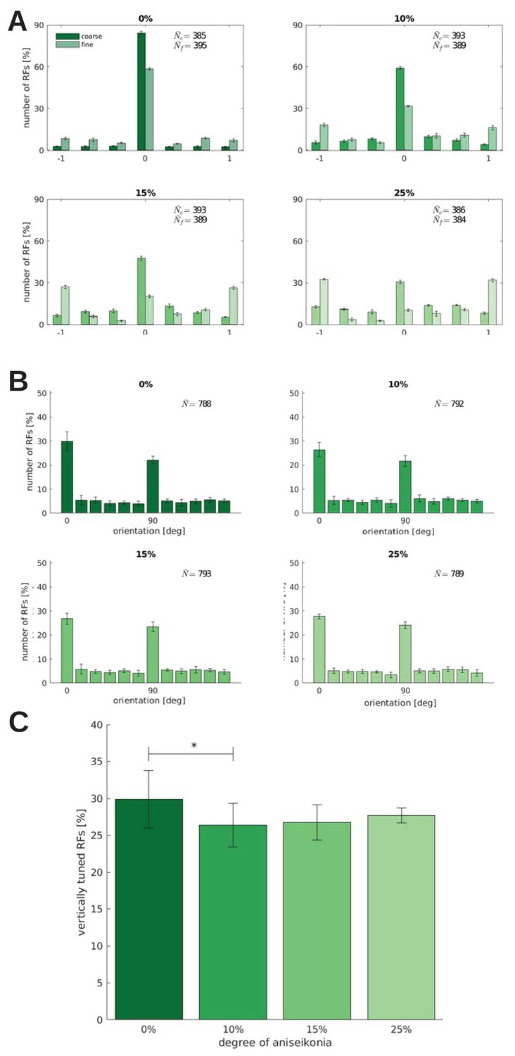
Binocularity, orientation tuning, and the number of RFs tuned to the vertical orientation for models trained under different degrees of aniseikonia.
Effect of different degrees of induced aniseikonia on (A) binocularity and (B) orientation tuning (over five random seeds). (C) depicts the number of cells tuned to the vertical orientation (0°). The difference between 0% and 10% aniseikonia is significant with a p-value of .
Figure 8—figure supplement 2
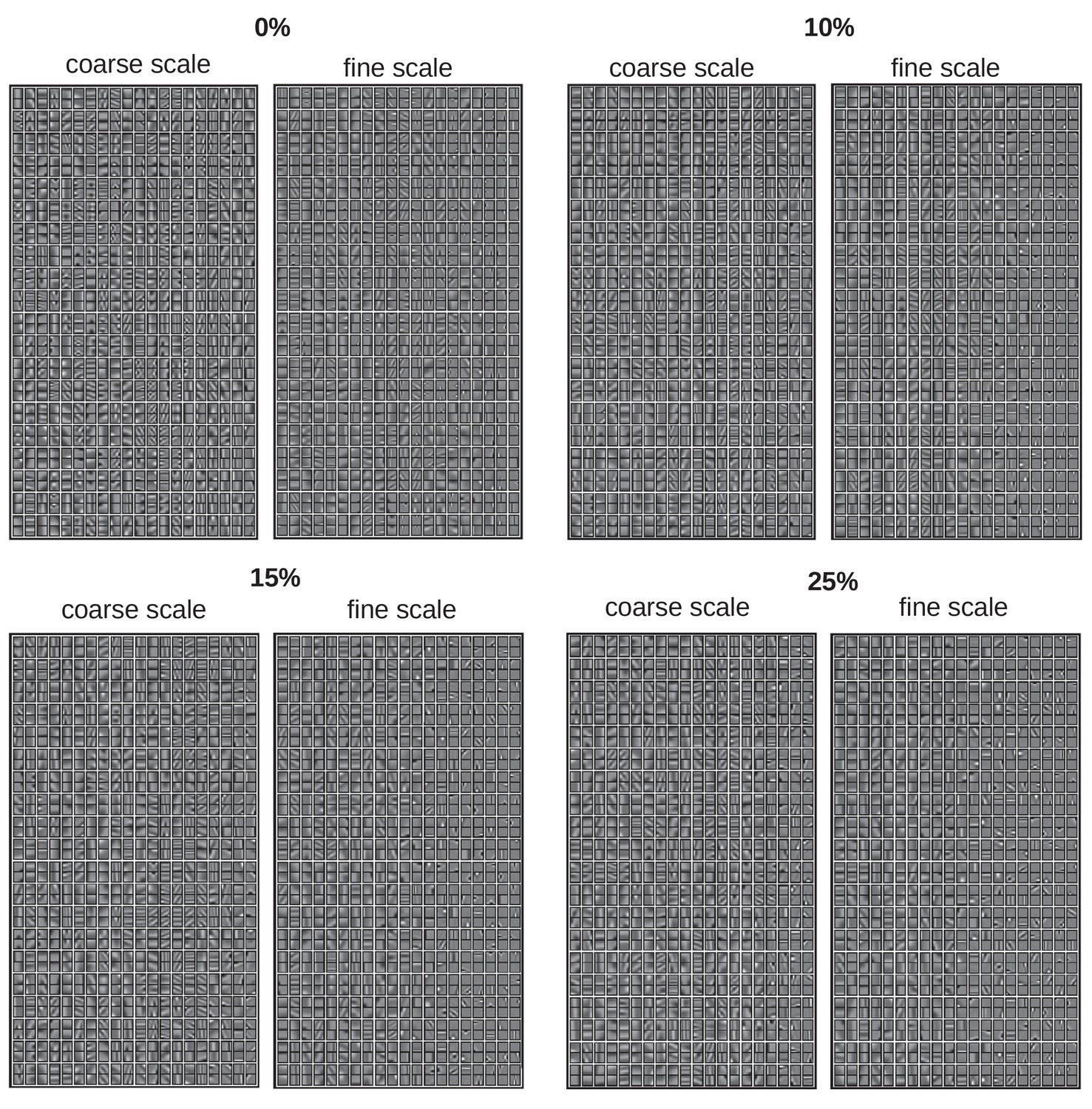
All RFs for different degrees of aniseikonia.
Full set of RFs from models trained under different degrees of aniseikonia.
Figure 9 with 1 supplement
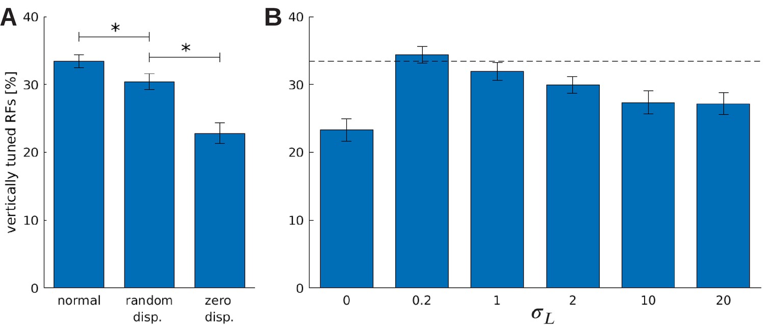
The effect of vergence learning on the number of neurons tuned to vertical orientations.
(A) Fraction of RFs tuned to vertical orientations for different versions of the model (see text for details). Asterisks indicate a statistically significant difference between the samples as revealed by a students t-test (p-values are and ). (B) Fractions of fine scale RFs tuned to vertical orientations for models trained with (truncated) Laplacian disparity distributions of different standard deviations . The value corresponds to 0 disparity all the time, while corresponds to an almost uniform disparity distribution. Error bars indicate the standard deviation over five different simulations. The black dotted line indicates the fraction of vertically tuned RFs in the normal model.
-
Figure 9—source data 1
Orientation tuning of the three different models. .
- https://cdn.elifesciences.org/articles/56212/elife-56212-fig9-data1-v2.zip
-
Figure 9—source data 2
Orientation tuning of models trained under different Laplacian disparity policies for coarse and fine scale.
- https://cdn.elifesciences.org/articles/56212/elife-56212-fig9-data2-v2.zip
Figure 9—figure supplement 1
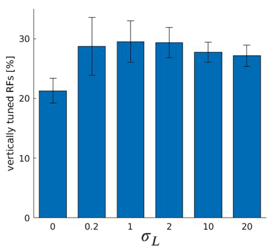
Number of RFs tuned to vertical orientations for coarse and fine scale combined.
Fractions of RFs tuned to vertical orientations for models trained with Laplacian disparity distributions of different standard deviations for coarse and fine scale combined.
Figure 10
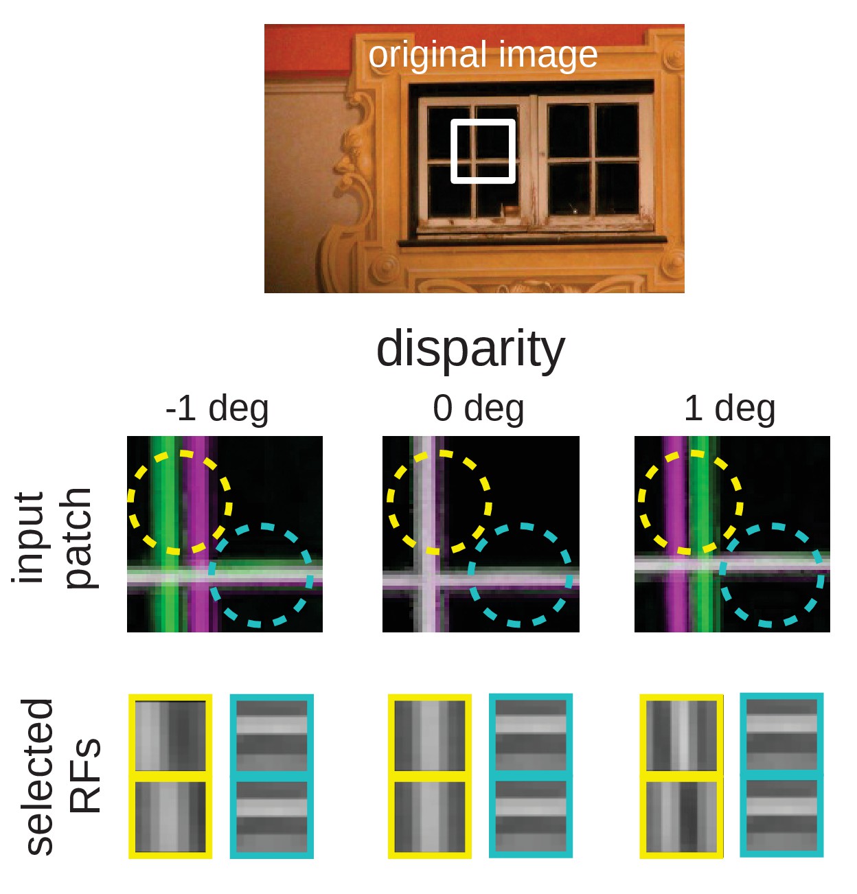
Intuition for the over-representation of vertical edges when different disparities have to be encoded.
Top: Input scence with marked input patch. Middle: Anaglyph rendering (left: green, right: magenta) of the patch for three different disparities. Two RF locations are highlighted (yellow and cyan circles). Bottom: RFs selected by the sparse coder to encode the inputs. While the RF that encodes the input in the cyan circle is the same for all disparities, the input inside the yellow circle can best be encoded by RFs that are tuned to the corresponding disparities.
Figure 11
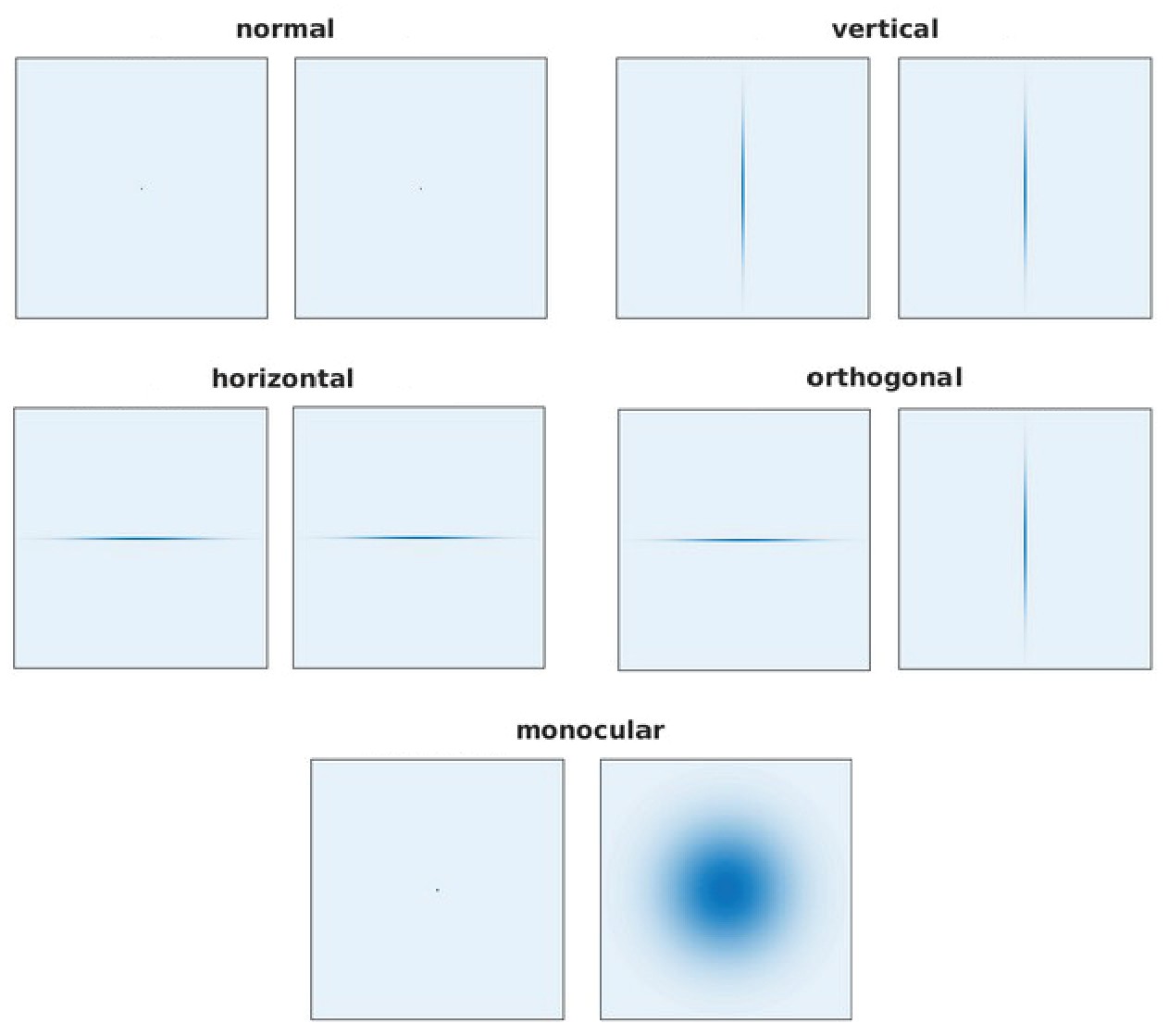
The filters used for the normal, vertical, horizontal, othogonal, and monocular models.
-
Figure 11—source data 1
The actual filters used during training.
- https://cdn.elifesciences.org/articles/56212/elife-56212-fig11-data1-v2.zip
Appendix 1—figure 1

Orientation tuning for five models trained with the man-made section or a random sample from the McGill database.
Appendix 1—figure 2
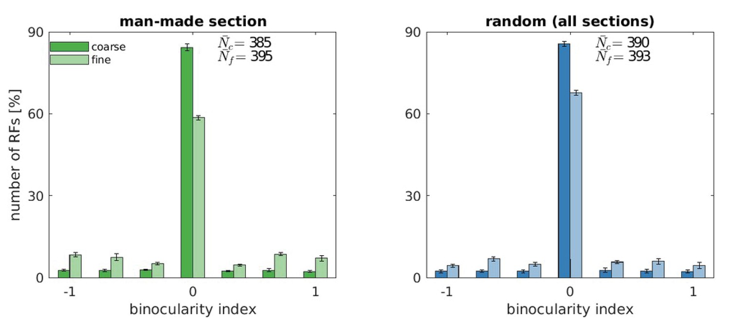
Binocularity values for five models trained with the man-made section or a random sample from the McGill database.
Appendix 1—figure 3
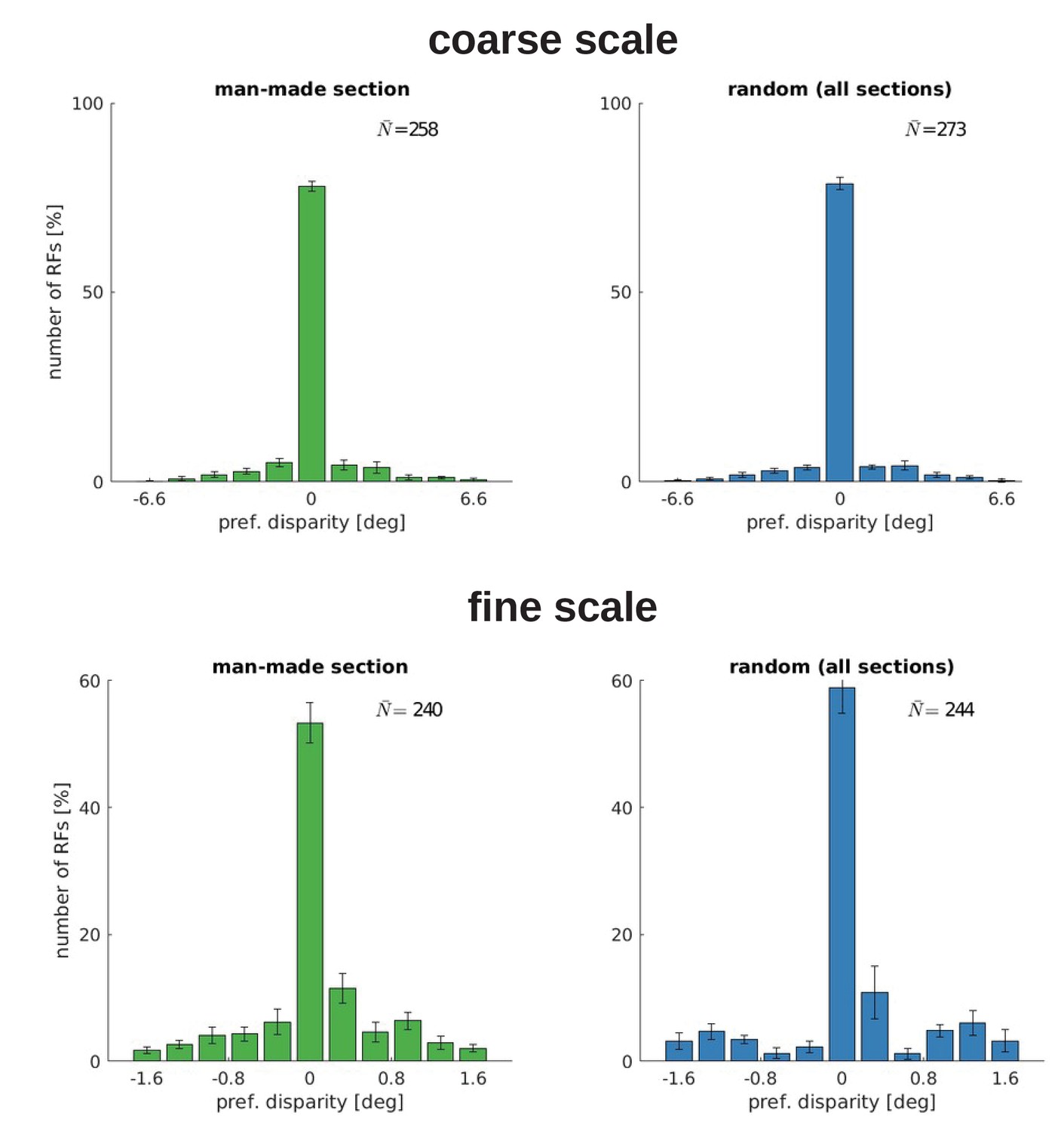
Disparity tuning for five models trained with the man-made section or a random sample from the McGill database.
Appendix 1—figure 4

Vergence acuity over training time (A) and at testing (B) for five models trained with the man-made section or a random sample from the McGill database.
Appendix 1—figure 5
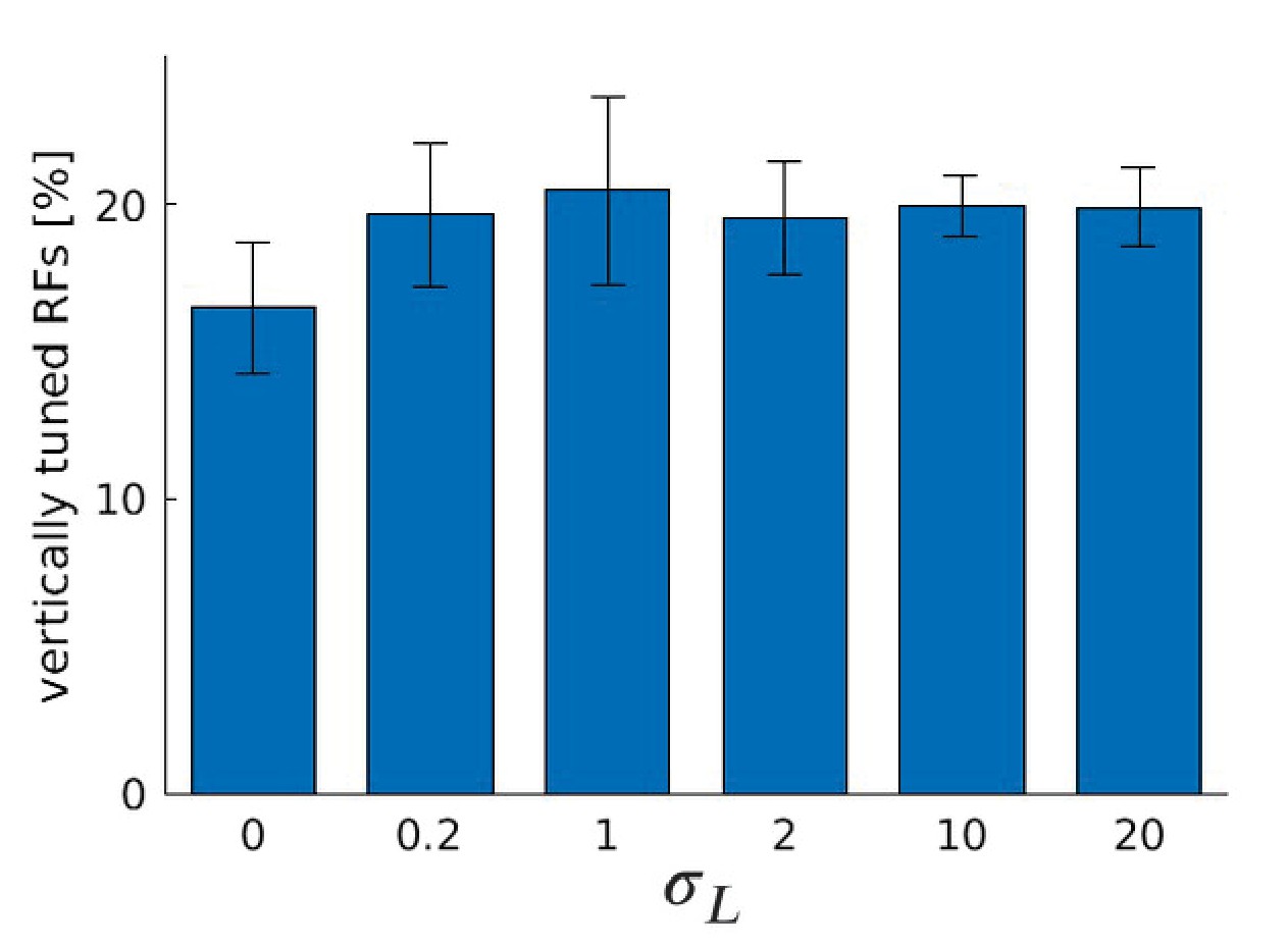
Number of RFs tuned to the vertical orientation for different values of , the standard deviation of the truncated Laplacian disparity input distribution, for five models trained with a random sample from the McGill database.
Compared to the man-made section in Figure 9B, we observe an increase in the number of RFs for small but non-zero values of and a decrease for bigger values of . However, the magnitude of the effect is reduced.
Appendix 2—figure 1
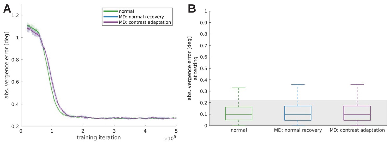
In response to the reviewers’ comments, we tested the effect that patching the weak eye would have on the recovery from monocular deprivation (Zhou et al., 2019).
To that end a model was trained under monocular deprivation, then normal visual input was reinstated and the weak eye received twice as much contrast as the other eye. This model, MD constrast adaptation, is compared to the normal and a reference model that did not receive an increased contrast (MD normal recovery), during training (A) and testing (B). All models trained under monocular deprivation can recover, when the RFs are still plastic. We do not observe a significant difference between the normal recovery and the contrast adaptation, probably because our model does not incorporate an interocular suppression mechanism that has been used to explain the effects of amblyopia on visual function (Zhou et al., 2018).
Videos
Video 1
Vergence performance for normal visual input.
The sizes of the scales and the according patch sizes are indicated in blue for the coarse scale and red for the fine scale.
Video 2
Vergence performance on a randomly generated set of RDS.
Additional files
Download links
A two-part list of links to download the article, or parts of the article, in various formats.
Downloads (link to download the article as PDF)
Open citations (links to open the citations from this article in various online reference manager services)
Cite this article (links to download the citations from this article in formats compatible with various reference manager tools)
The development of active binocular vision under normal and alternate rearing conditions
eLife 10:e56212.
https://doi.org/10.7554/eLife.56212


