Interrogating theoretical models of neural computation with emergent property inference
- Department of Neuroscience, Columbia University, United States
- Princeton Neuroscience Institute, United States
- Princeton University, United States
- Allen Institute for Brain Science, United States
- Institute of Neuroscience, Chinese Academy of Sciences, China
- Howard Hughes Medical Institute, United States
- Department of Statistics, Columbia University, United States
Figures
Figure 1 with 4 supplements
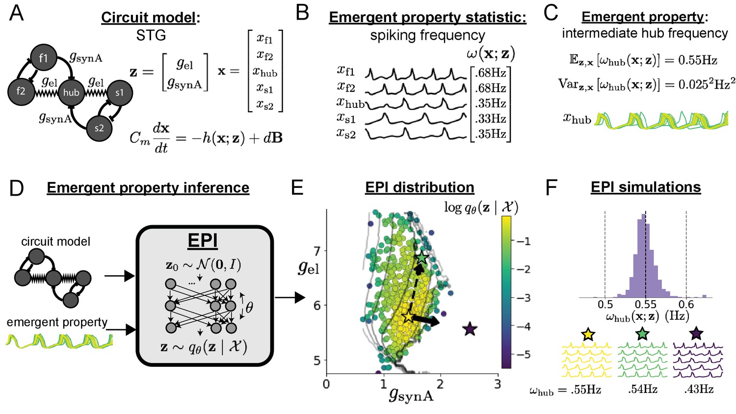
Emergent property inference in the stomatogastric ganglion.
(A) Conductance-based subcircuit model of the STG. (B) Spiking frequency is an emergent property statistic. Simulated at nS and nS. (C) The emergent property of intermediate hub frequency. Simulated activity traces are colored by log probability of generating parameters in the EPI distribution (Panel E). (D) For a choice of circuit model and emergent property, EPI learns a deep probability distribution of parameters . (E) The EPI distribution producing intermediate hub frequency. Samples are colored by log probability density. Contours of hub neuron frequency error are shown at levels of 0.525, 0.53, … 0.575 Hz (dark to light gray away from mean). Dimension of sensitivity (solid arrow) and robustness (dashed arrow). (F) (Top) The predictions of the EPI distribution. The black and gray dashed lines show the mean and two standard deviations according the emergent property. (Bottom) Simulations at the starred parameter values.
Figure 1—figure supplement 1
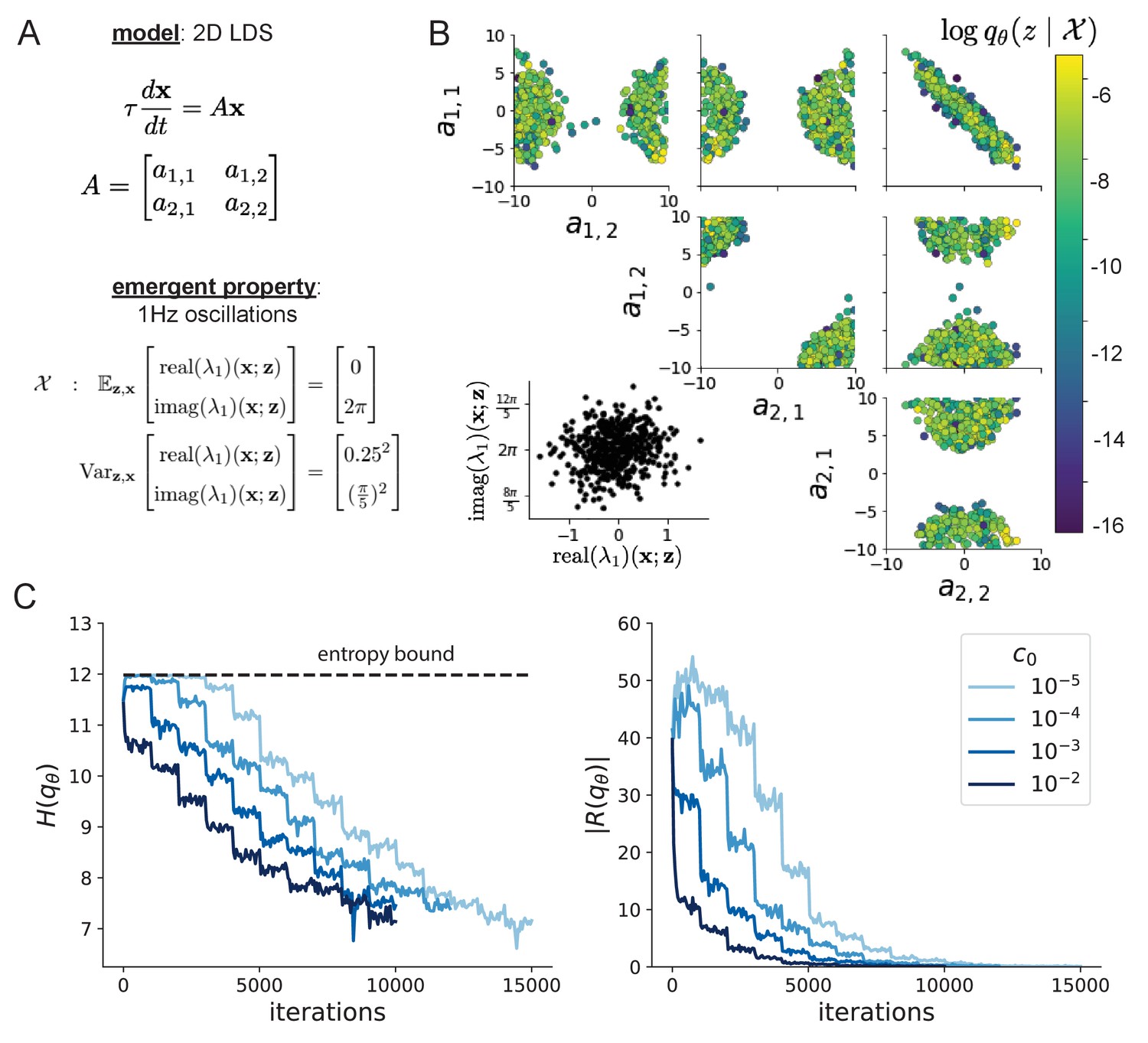
Emergent property inference in a 2D linear dynamical system.
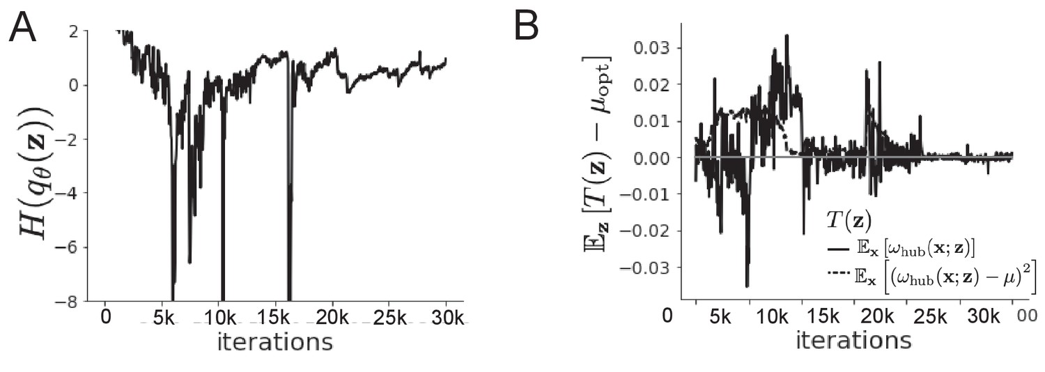
(A) Two-dimensional linear dynamical system model, where real entries of the dynamics matrix are the parameters. (B) The EPI distribution for a two-dimensional linear dynamical system with that produces an average of 1 Hz oscillations with some small amount of variance. Dashed lines indicate the parameter axes. (C) Entropy throughout the optimization. At the beginning of each augmented lagrangian epoch ( iterations), the entropy dipped due to the shifted optimization manifold where emergent property constraint satisfaction is increasingly weighted. (D) Emergent property moments throughout optimization. At the beginning of each augmented lagrangian epoch, the emergent property moments adjust closer to their constraints.
Figure 1—figure supplement 2
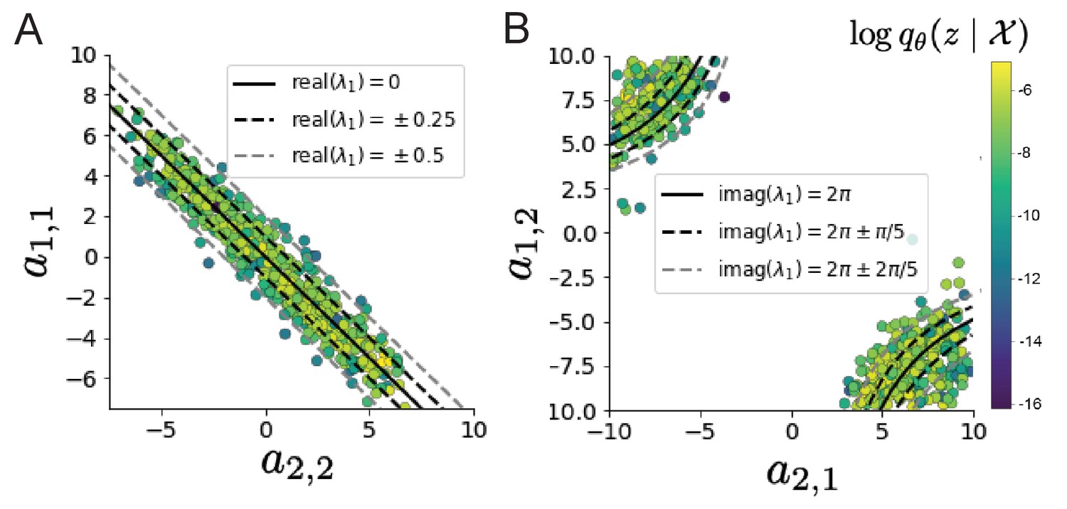
Analytic contours of inferred EPI distribution.
(A) Probability contours in the - plane were derived from the relationship to emergent property statistic of growth/decay factor . (B) Probability contours in the - plane were derived from the emergent property statistic of oscillation frequency .
Figure 1—figure supplement 3
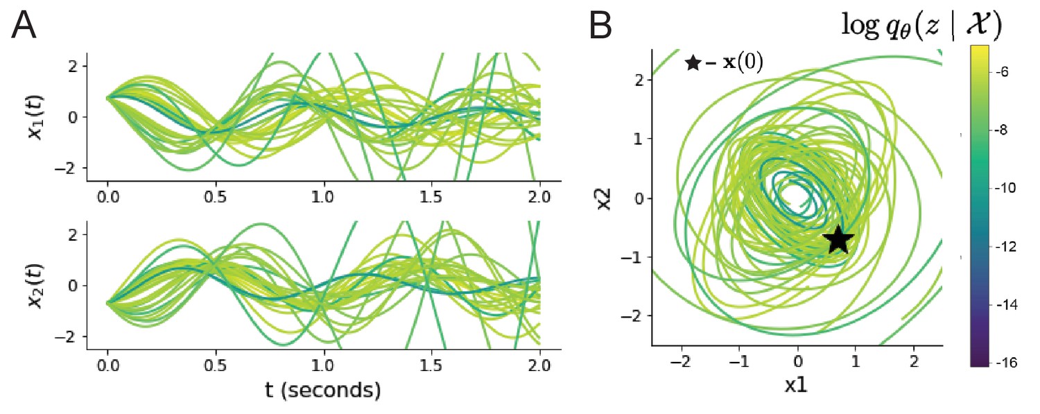
Sampled dynamical systems and their simulated activity from colored by log probability.
(A) Each dimension of the simulated trajectories throughout time. (B) The simulated trajectories in phase space.
Figure 1—figure supplement 4
EPI optimization of the STG model producing network syncing.
(A) Entropy throughout optimization. (B) The emergent property statistic means and variances converge to their constraints at 25,000 iterations following the fifth augmented lagrangian epoch.
Figure 2 with 3 supplements
Inferring recurrent neural networks with stable amplification.
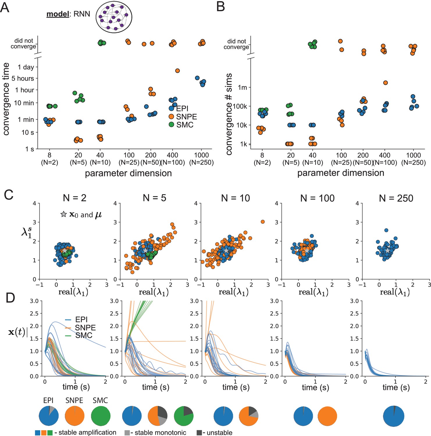
(A) Wall time of EPI (blue), SNPE (orange), and SMC-ABC (green) to converge on RNN connectivities producing stable amplification. Each dot shows convergence time for an individual random seed. For reference, the mean wall time for EPI to achieve its full constraint convergence (means and variances) is shown (blue line). (B) Simulation count of each algorithm to achieve convergence. Same conventions as A. (C) The predictive distributions of connectivities inferred by EPI (blue), SNPE (orange), and SMC-ABC (green), with reference to (gray star). (D) Simulations of networks inferred by each method (). Each trace (15 per algorithm) corresponds to simulation of one . (Below) Ratio of obtained samples producing stable amplification, stable monotonic decay, and instability.
Figure 2—figure supplement 1
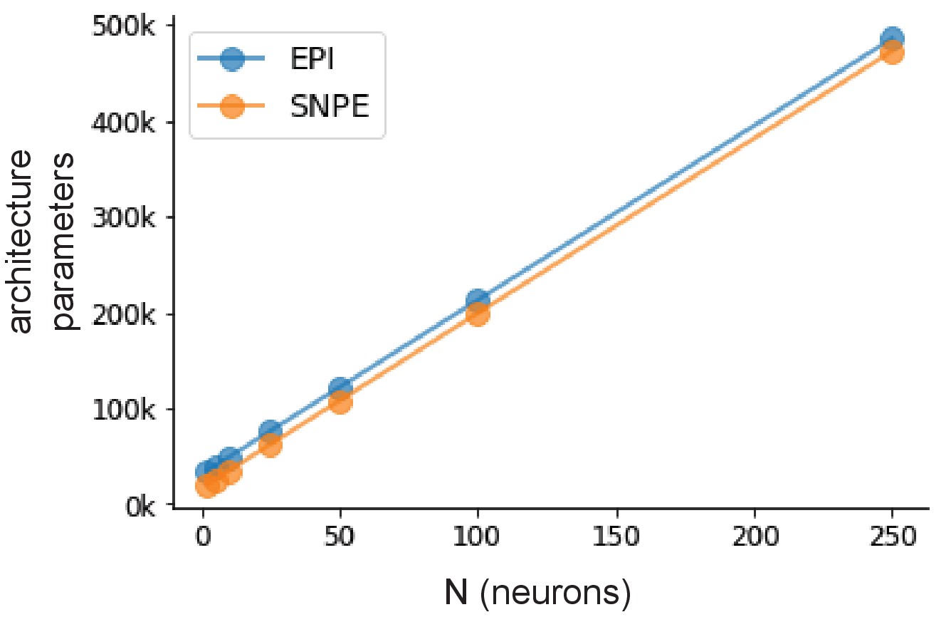
Architecture parameter comparison of EPI and SNPE.
Number of parameters in deep probability distribution architectures of EPI (blue) and SNPE (orange) by RNN size ().
Figure 2—figure supplement 2
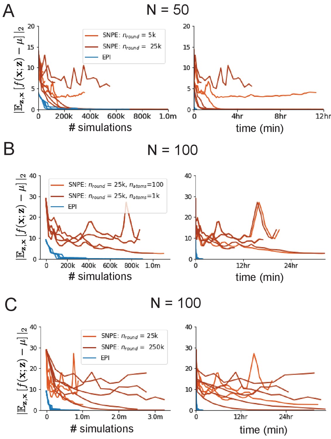
SNPE convergence was enabled by increasing , not .
(A) Difference of mean predictions throughout optimization at with by simulation count (left) and wall time (right) of SNPE with (light orange), SNPE with (dark orange), and EPI (blue). Each line shows an individual random seed. (B) Same conventions as A at of SNPE with (light orange) and (dark orange). (C) Same conventions as A at of SNPE with (light orange) and (dark orange).
Figure 2—figure supplement 3
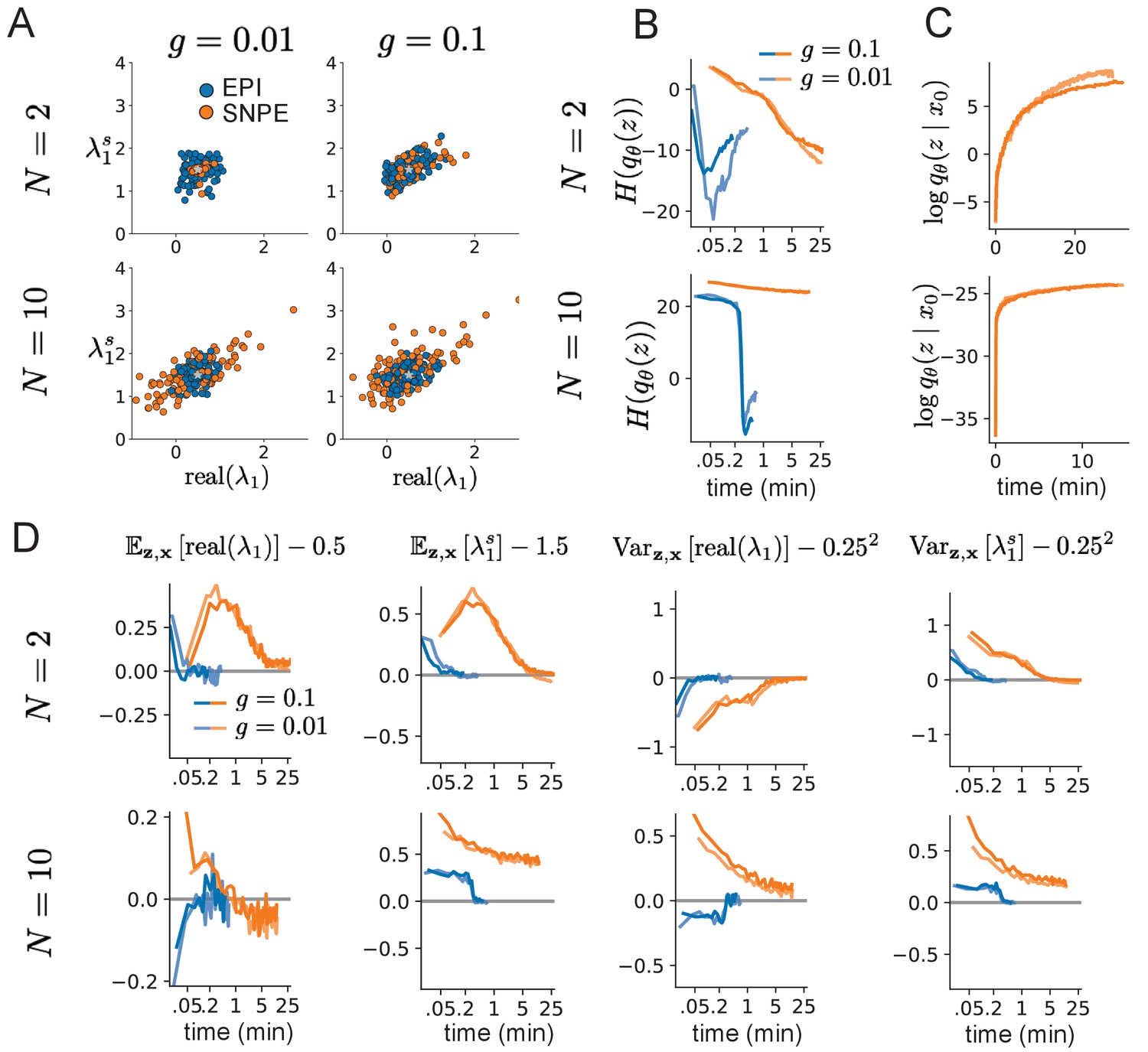
Model characteristics affect predictions of posteriors inferred by SNPE, while predictions of parameters inferred by EPI remain fixed.
(A) Predictive distribution of EPI (blue) and SNPE (orange) inferred connectivity of RNNs exhibiting stable amplification with (top), (bottom), (left), and (right). (B) Entropy of parameter distribution approximations throughout optimization with (top), (bottom), (dark shade), and (light shade). (C) Validation log probabilities throughout SNPE optimization. Same conventions as B. (D) Adherence to EPI constraints. Same conventions as B.
Figure 3 with 4 supplements
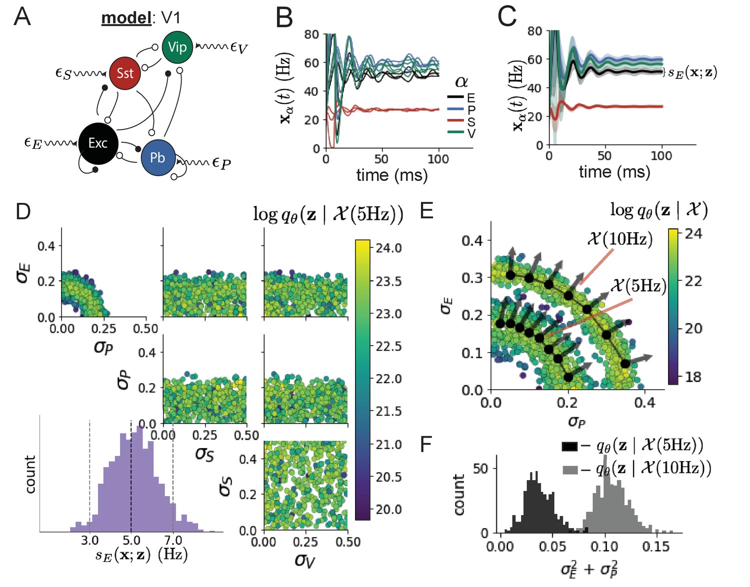
Emergent property inference in the stochastic stabilized supralinear network (SSSN).
(A) Four-population model of primary visual cortex with excitatory (black), parvalbumin (blue), somatostatin (red), and VIP (green) neurons (excitatory and inhibitory projections filled and unfilled, respectively). Some neuron-types largely do not form synaptic projections to others (). Each neural population receives a baseline input , and the E- and P-populations also receive a contrast-dependent input . Additionally, each neural population receives a slow noisy input . (B) Transient network responses of the SSSN model. Traces are independent trials with varying initialization and noise . (C) Mean (solid line) and standard deviation (shading) across 100 trials. (D) EPI distribution of noise parameters conditioned on E-population variability. The EPI predictive distribution of is show on the bottom-left. (E) (Top) Enlarged visualization of the - marginal distribution of EPI and . Each black dot shows the mode at each . The arrows show the most sensitive dimensions of the Hessian evaluated at these modes. (F) The predictive distributions of of each inferred distribution and .
Figure 3—figure supplement 1
EPI inferred distribution for .
Figure 3—figure supplement 2
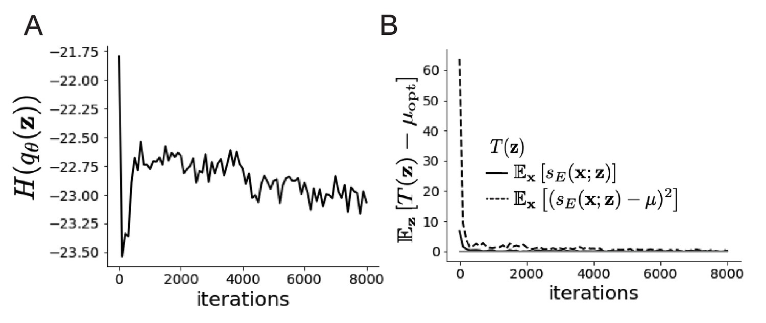
EPI optimization.
(A) Entropy throughout optimization. (B) The emergent property statistic means and variances converge to their constraints at 8000 iterations following the fourth augmented lagrangian epoch.
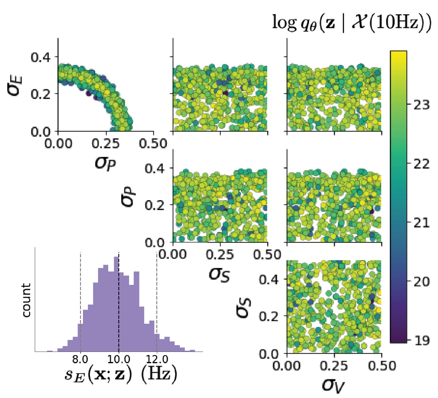
Figure 3—figure supplement 3

EPI predictive distributions of the sum of squares of each pair of noise parameters.
Figure 3—figure supplement 4

SSSN simulations for small increases in neuron-type population input (left); average (solid) and standard deviation (shaded) of stochastic fluctuations of responses (right).
Figure 4 with 5 supplements
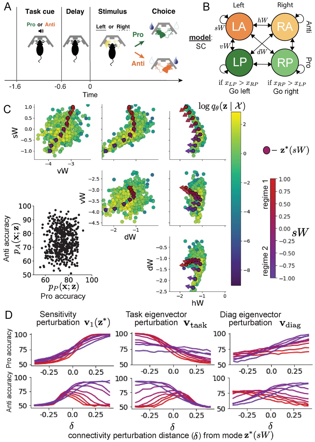
Inferring rapid task switching networks in superior colliculus.
(A) Rapid task switching behavioral paradigm (see text). (B) Model of superior colliculus (SC). Neurons: LP - Left Pro, RP - Right Pro, LA - Left Anti, RA - Right Anti. Parameters: - self, - horizontal, -vertical, - diagonal weights. (C) The EPI inferred distribution of rapid task switching networks. Red/purple parameters indicate modes colored by . Sensitivity vectors are shown by arrows. (Bottom-left) EPI predictive distribution of task accuracies. (D) Mean and standard error ( = 25, bars not visible) of accuracy in Pro (top) and Anti (bottom) tasks after perturbing connectivity away from mode along (left), (middle), and (right).
Figure 4—figure supplement 1
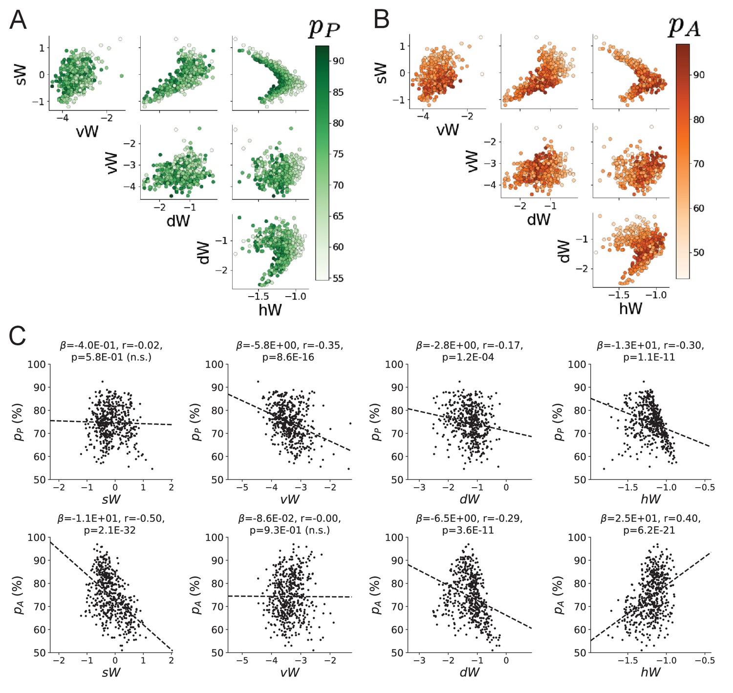
Task accuracy by EPI inferred SC network connectivity.
(A) Same pairplot as Figure 4C colored by Pro-task accuracy. (B) Same as A colored by Anti-task accuracy. (C) Connectivity parameters of EPI distributions versus task accuracies. β is slope coefficient of linear regression, is correlation, and is the two-tailed p-value.
Figure 4—figure supplement 2

SC network simulations by regime.
(A) Simulations in network regime 1: . (B) Simulations in network regime 2: .
Figure 4—figure supplement 3
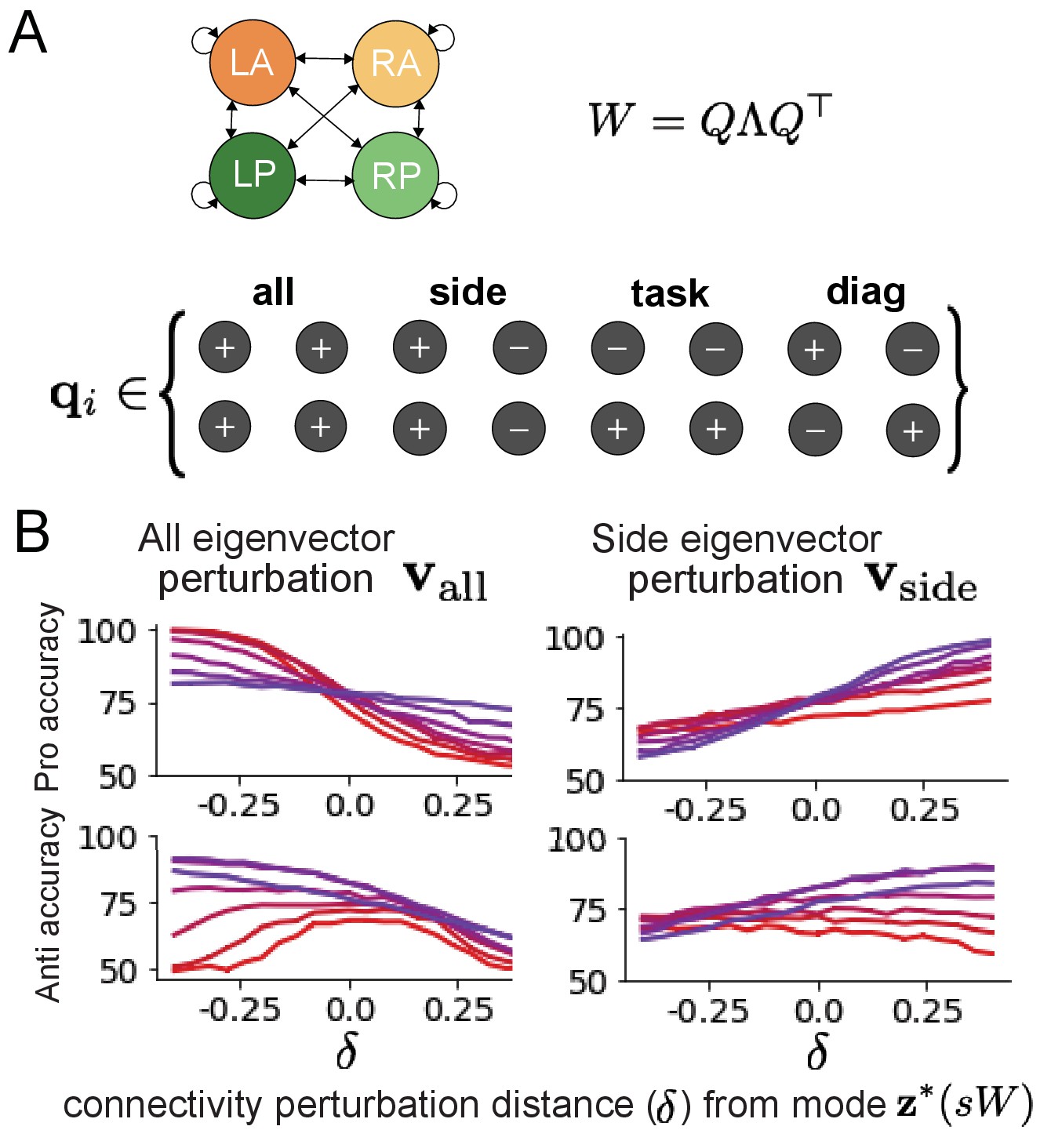
Eigenmodes of SC connectivity.
(A) Invariant eigenvectors of connectivity matrix . (B) Accuracies for connectivity perturbations when changing and ( and shown in Figure 4D).
Figure 4—figure supplement 4

EPI optimization of the SC model producing rapid task switching.
(A) Entropy throughout optimization. (B) The emergent property statistic means and variances converge to their constraints at 20,000 iterations following the tenth augmented lagrangian epoch.
Figure 4—figure supplement 5
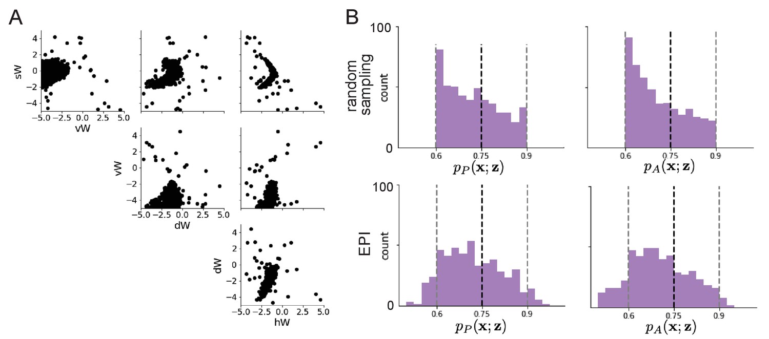
SC connectivities obtained through brute-force sampling.
(A) Rapid task switching SC connectivities obtained from random sampling. (B) Task accuracies of the inferred distributions from random sampling (top) and EPI (bottom).
Figure 5 with 2 supplements
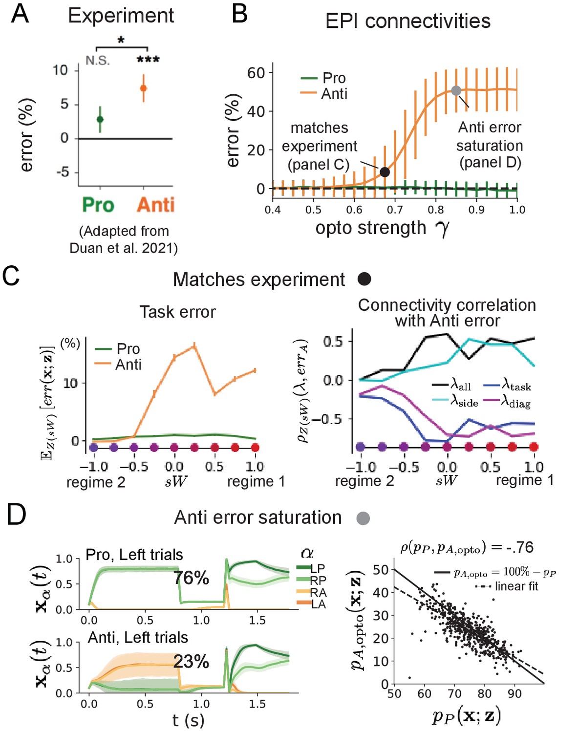
Responses to optogenetic perturbation by connectivity regime.
(A) Mean and standard error (bars) across recording sessions of task error following delay period optogenetic inactivation in rats. (B) Mean and standard deviation (bars) of task error induced by delay period inactivation of varying optogenetic strength γ across the EPI distribution. (C) (Left) Mean and standard error of Pro and Anti error from regime 1 to regime 2 at . (Right) Correlations of connectivity eigenvalues with Anti error from regime 1 to regime 2 at . (D) (Left) Mean and standard deviation (shading) of responses of the SC model at the mode of the EPI distribution to delay period inactivation at . Accuracy in Pro (top) and Anti (bottom) task is shown as a percentage. (Right) Anti-accuracy following delay period inactivation at versus accuracy in the Pro-task across connectivities in the EPI distribution.
Figure 5—figure supplement 1
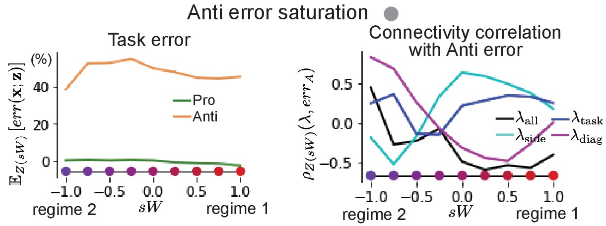
SC responses to delay period inactivation at Anti error saturating levels.
(Left) Mean and standard error of Pro- and Anti-error from regime 1 to regime 2 at .
(Right) Correlations of connectivity eigenvalues with Anti-error from regime 1 to regime 2 at .
Figure 5—figure supplement 2
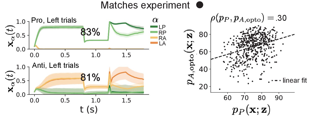
SC responses to delay period inactivation at experiment matching levels.
(Left) Mean and standard deviation (shading) of responses of the SC model at the mode of the EPI distribution to delay period inactivation at .
Accuracy in Pro (top) and Anti (bottom) task is shown as a percentage. (Right) Anti-accuracy following delay period inactivation at versus accuracy in the Pro-task across connectivities in the EPI distribution.
Additional files
Download links
A two-part list of links to download the article, or parts of the article, in various formats.
Downloads (link to download the article as PDF)
Open citations (links to open the citations from this article in various online reference manager services)
Cite this article (links to download the citations from this article in formats compatible with various reference manager tools)
Interrogating theoretical models of neural computation with emergent property inference
eLife 10:e56265.
https://doi.org/10.7554/eLife.56265


