Figures and data in Evolution of multicellularity by collective integration of spatial information

Figures
Videos
Tables
Additional files

21 figures, 7 videos, 1 table and 1 additional file

Figures

Figure 1

Download asset Open asset

Model description.

(a) Adhesion between two cells is mediated by receptors and ligands (represented by a bitstring, see Hogeweg, 2000). The receptor of one cell is matched to the ligand of the other cell and vice versa. The more complementary the receptors and ligands are, the lower the J values and the stronger the adhesion between the cells. (b) Persistent migration is implemented by endowing each cell with a preferred direction of motion ${\vec{v}}_{p}$ . Every $τ_{p}$ MCS, this direction is updated with a cell’s actual direction of motion in that period. (c) The chemoattractant gradient in the lattice. The lines and colour indicate equal amounts of chemoattractant. Note the scattered empty lattice sites. (d) A cell can only sense the chemoattractant in the lattice sites that correspond to its own location. The cell will then move preferentially in the direction of perceived higher concentration, the chemotaxis vector. This vector points from the cell’s centre of mass to the centre of mass of the chemoattractant detected by the cell (the blue dot).

Figure 2

Download asset Open asset

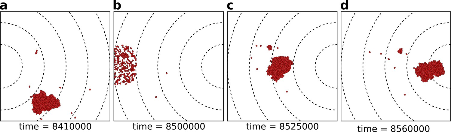
The eco-evolutionary setup of the model.

(a) A population of $N = 200$ cells moves by chemotaxis towards the peak of the gradient, which in this season is located at the left boundary of the grid. (b) At the end of the season, cells divide, the population excess is killed randomly, and the direction of the chemotactic signal is changed, after which the new season begins (**c, d**). The snapshots are taken at the indicated time points from a simulation where a season lasts $τ_{s} = 100 \times 10^{3}$ MCS. Dashed lines in the snapshots are gradient isoclines.

Figure 3

Download asset Open asset

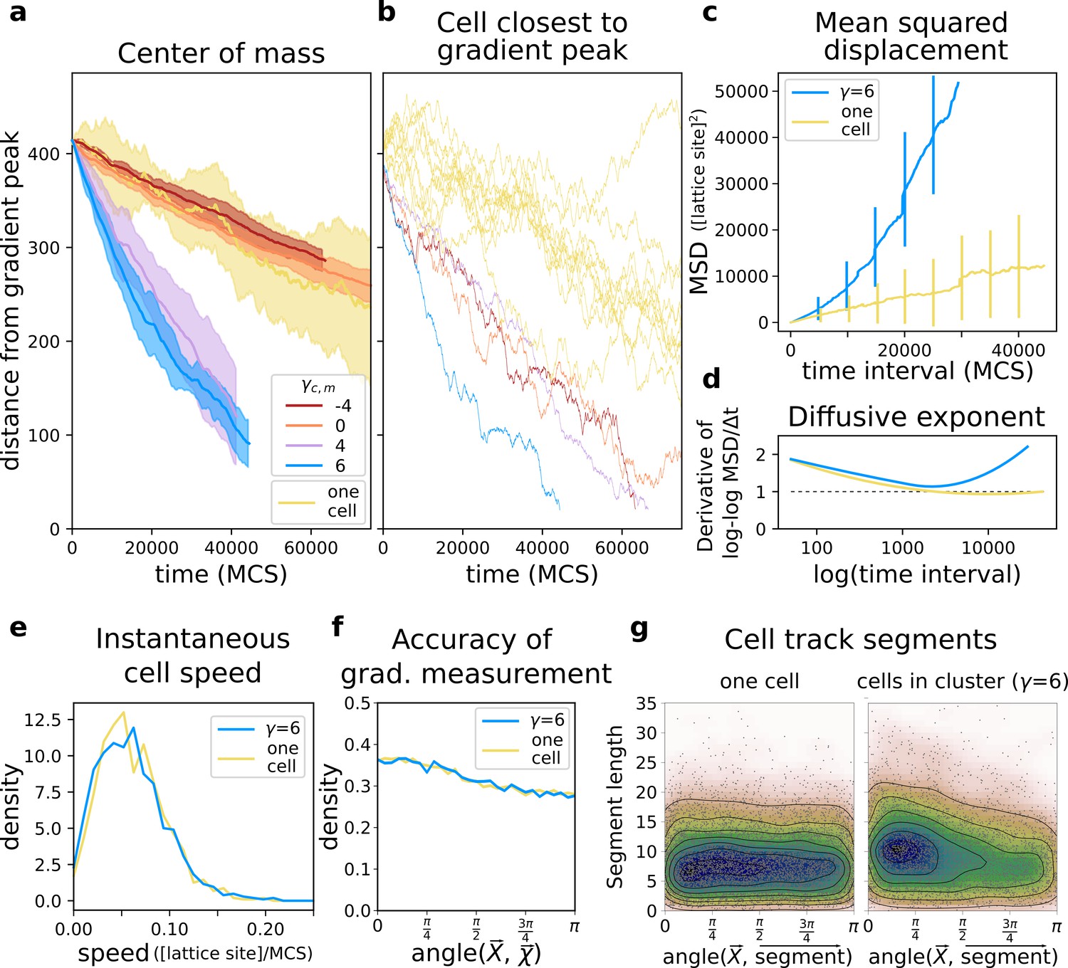
A group of cells performs chemotaxis efficiently in a noisy shallow gradient.

(a) Distance of the centre of mass of $N = 50$ cells from the peak of the gradient as a function of time, for different values of $γ \in [- 4, 6]$ (five independent runs for each value), together with the average position of 10 isolated cells (i.e. from simulations with only one cell). (b) The position of the cell closest to the gradient origin as a function of time (taken from the same simulations as in a), and the positions of 10 individual cells (whose average generates the corresponding plot in a). (c) Mean square displacement (MSD) per time interval for two datasets each with 50 simulations of either single cells or clusters of strongly adhering cells ( $N = 50$ , $γ = 6$ ), in which case we extracted one cell per simulation. These data sets were also used for the following plots. (d) Diffusive exponent extracted from the MSD plot, obtained from the log-log transformed MSD plots by fitting a smoothing function and taking its derivative (Appendix 1.1). (e) Distribution of instantaneous cell speeds (f) Distribution of angles between cells’ measurement of the gradient $\vec{χ}$ , and the actual direction of the gradient peak $\vec{X}$ , as measured from the position of the cell. (g) The length of straight segments in cell tracks vs. their angle with the actual gradient direction. Each point represents one segment of a cell’s trajectory. To extract these straight segments a simple algorithm was used (Appendix 1.8). Contour lines indicate density of data points.

Figure 4

Download asset Open asset

Indivdual cell trajectories are noisy, also within a cluster.

(a) The movement of a single cell. (b) Typical movement of a cluster of strongly adhering cells, and of the cells inside the cluster. Cells are placed on the right of the field and move towards higher concentration of the gradient (to the left of the field). Dashed lines are gradient isoclines.

Figure 5

Download asset Open asset

The evolution of multicellularity.

(a) Multicellularity ( $γ > 0$ ) rapidly evolves in a population of $N = 200$ cells with $τ_{s} = 10^{5}$ . (b) Multicellularity only evolves when seasons are sufficiently long $τ_{s} \geq 50 * 10^{3}$ ; unicellular strategies evolve when seasons are short $τ_{s} \leq 10 * 10^{3}$ , and both strategies are viable depending on initial conditions for intermediate values of $τ_{s}$ . The dashed line indicates the separatrix between the basins of attraction of the two evolutionary steady states; it is estimated as the mid-point where evolutionary simulations with consecutive initial values of $γ \in {- 6, - 4, - 2, 0, 2, 4, 6}$ evolve to alternative steady states. In both panes, $⟨ ⟨ γ ⟩ ⟩$ is estimated as $⟨ J_{c, m} ⟩ - ⟨ J_{c, c} ⟩ / 2$ , where $⟨ J_{c, c} ⟩$ and $⟨ J_{c, m} ⟩$ are calculated from the $J_{c, c}$ and $J_{c, m}$ extracted from the system at evolutionary steady state. The initial J values, indicated by the dotted lines, are such that $γ = 0$ . (c) Snapshots of the spatial distribution of the population at evolutionary steady state for $τ_{s} = 20 \cdot 10^{3}$ and $τ_{s} = 100 \cdot 10^{3}$ MCS.

Figure 6

Download asset Open asset

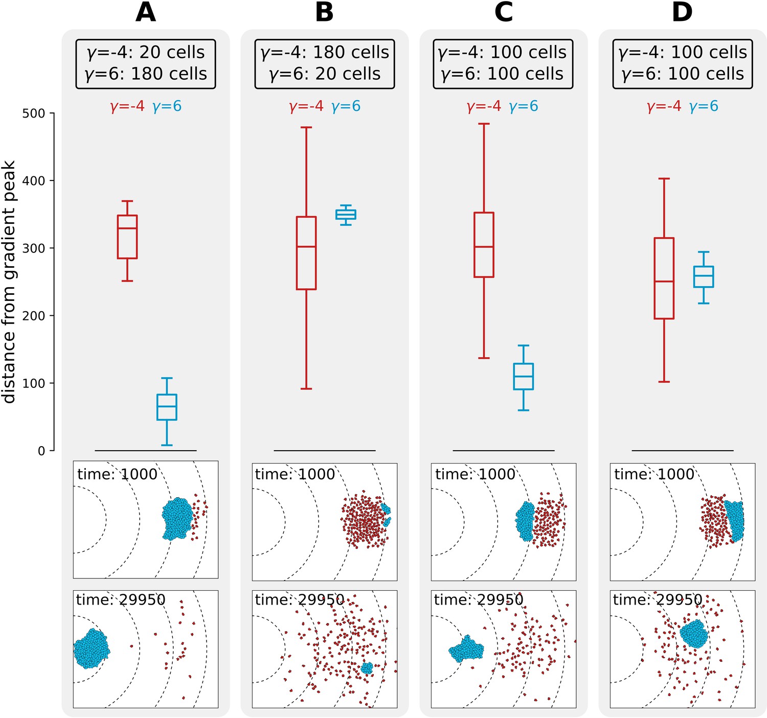
Interference competition between adhering and non-adhering cells explains evolutionary bistability.

We let a simulation run for $τ_{s} = 30 \times 10^{3}$ MCS and then record the distance from the peak of the gradient, for two different populations of cells - one non-adhering (in red, $γ = - 4$ ) and one adhering (in blue, $γ = 6$ ), for different initial conditions. The snapshots underneath are the initial and final spatial configurations of the cells on the grid. (A) 180 adhering and 20 non-adhering cells, placed so that the adhering cells are closer to the source of the gradient; (B) 20 adhering and 180 non-adhering cells, placed so that the non-adhering cells are closer to the source of the gradient; (C) 100 adhering and 100 non-adhering cells, placed so that the adhesive ones are closer to the source of the gradient; (D) 100 adhering and 100 non-adhering cells, placed so that the non-adhering cells are closer to the source of the gradient. Dashed lines in the snapshots are gradient isoclines.

Appendix 1—figure 1

Download asset Open asset

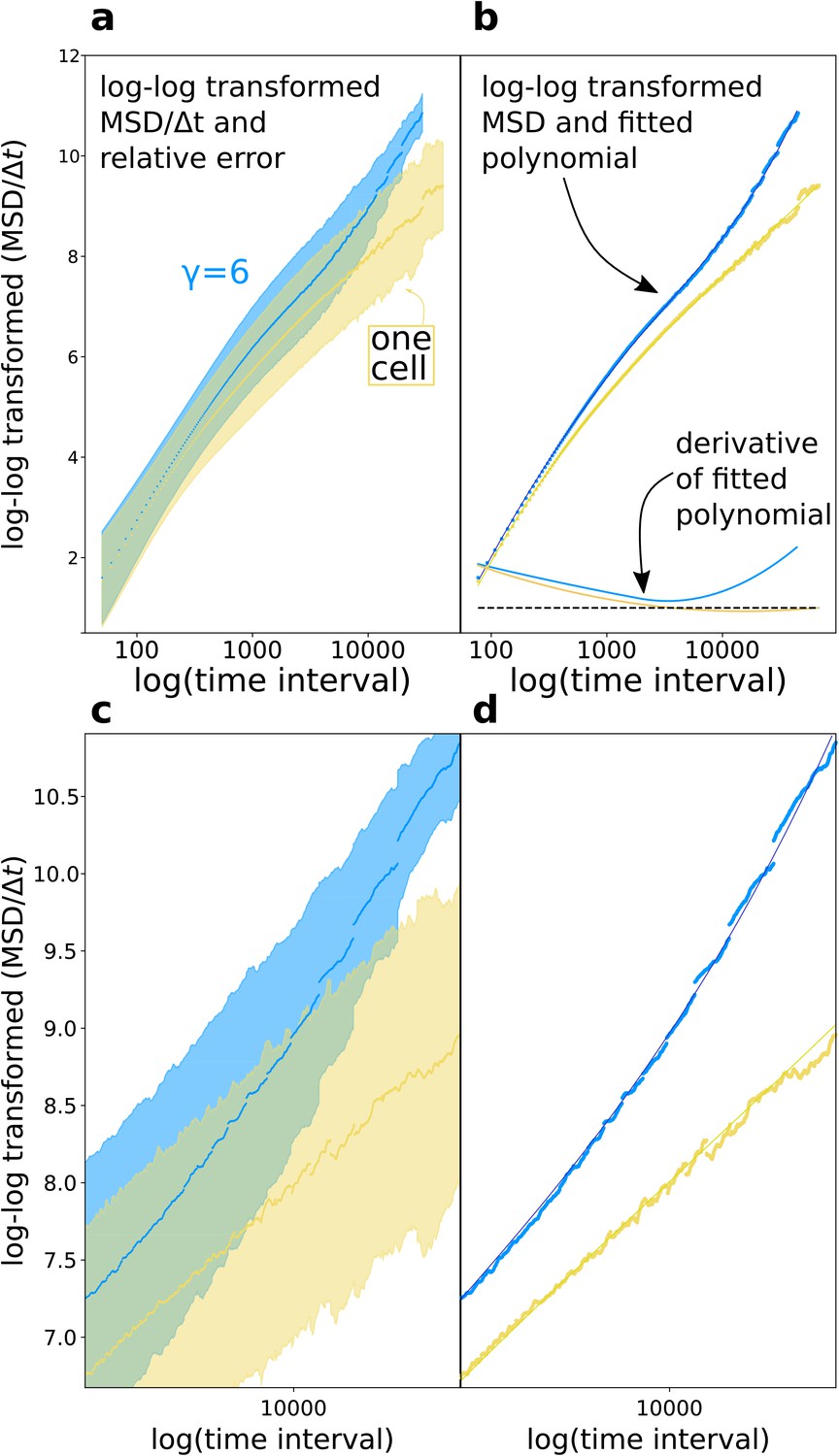
Diffusion exponent approximation.

(a) We log-log transformed the data (the shaded area is the relative error $Var (MSD (Δ t)) / MSD (Δ t)$ ). (b) We fitted a polynomial function to the data, then took the derivative of the polynomial function. (**c,d**) Magnifications of respectively (a) and (b).

Appendix 1—figure 2

Download asset Open asset

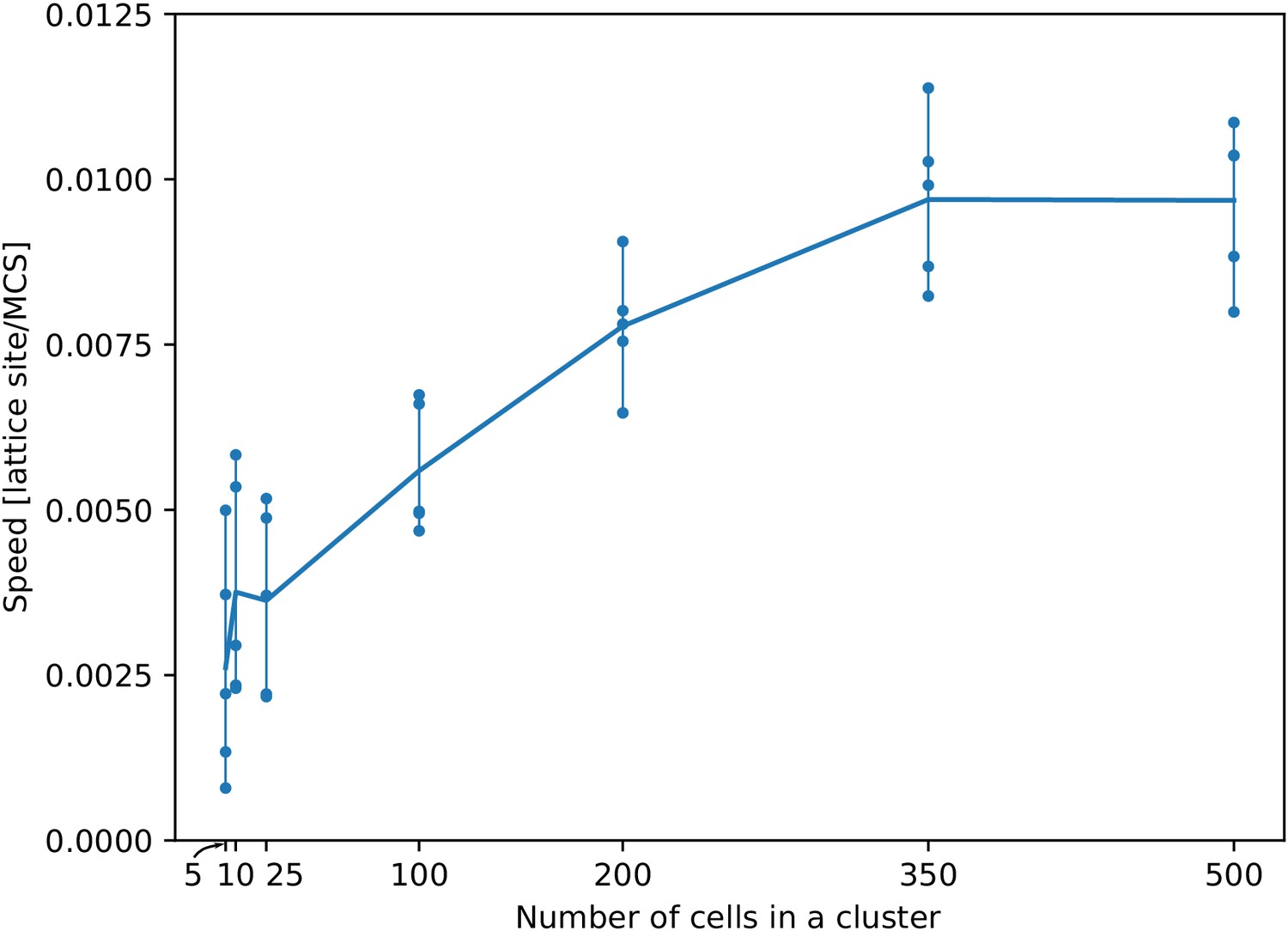
The speed of a cluster towards the peak of the gradient saturates with larger cluster sizes.

For each cluster size, we ran five independent simulations. Each dot corresponds to one simulation. Their average (per cluster size) generates the line. All other parameters as in main text.

Appendix 1—figure 3

Download asset Open asset

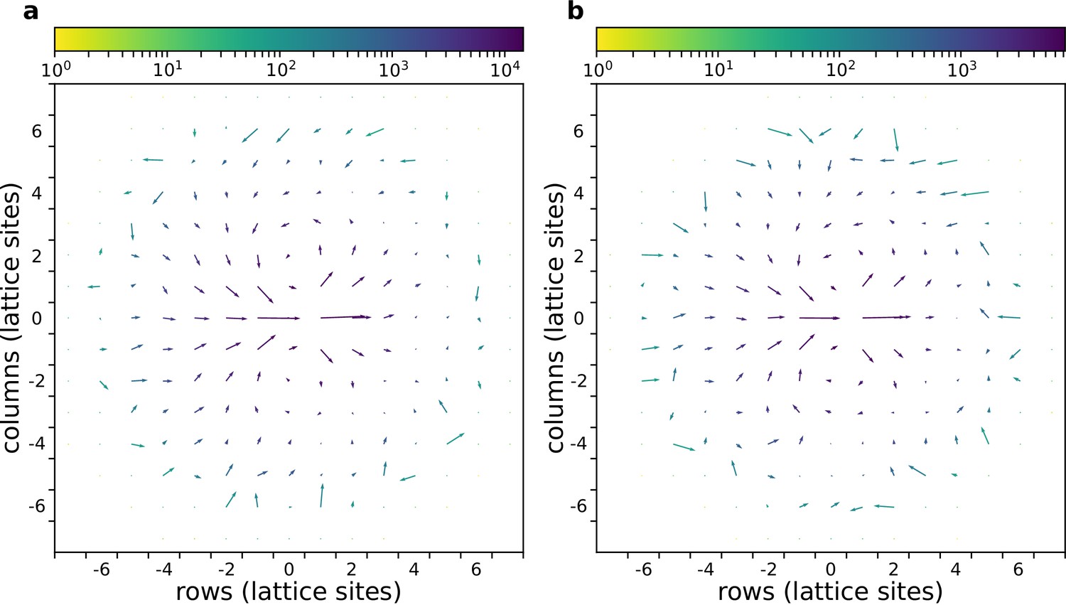
The flow field of a cluster of cells with and without gradient.

(a) With chemoattractant gradient. (b) Without chemoattractant gradient. In both cases $N = 50$ cells with $γ = 6$ are placed at the centre of the field (All other parameters as in main text).

Appendix 1—figure 4

Download asset Open asset

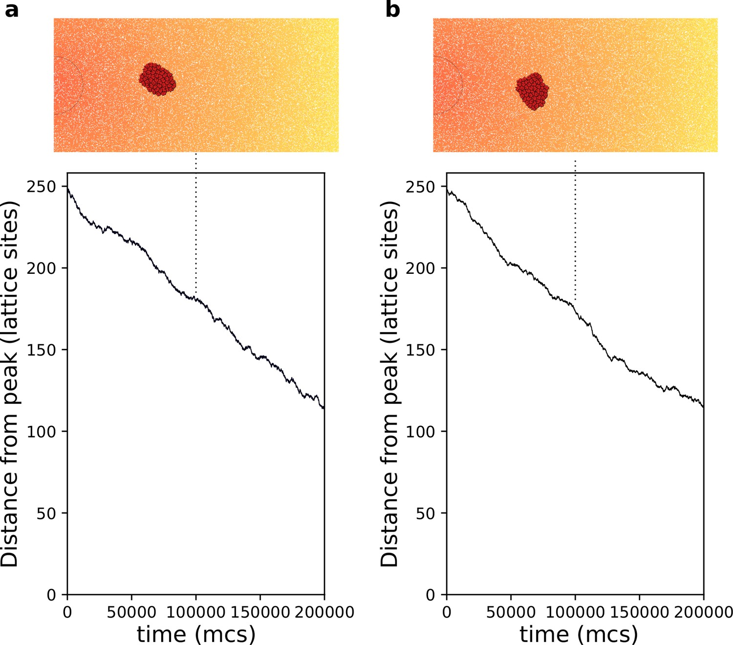
Chemotaxis of a rigid cluster.

(a) $τ_{p} = 5$ . (b) $μ_{p} = 0.5$ . In both cases $N = 50$ cells with $γ = 6$ are placed on the right of the field and move towards higher concentration of the gradient (the semicircle indicates the resource location, where the gradient is highest. All other parameters as in main text).

Appendix 1—figure 5

Download asset Open asset

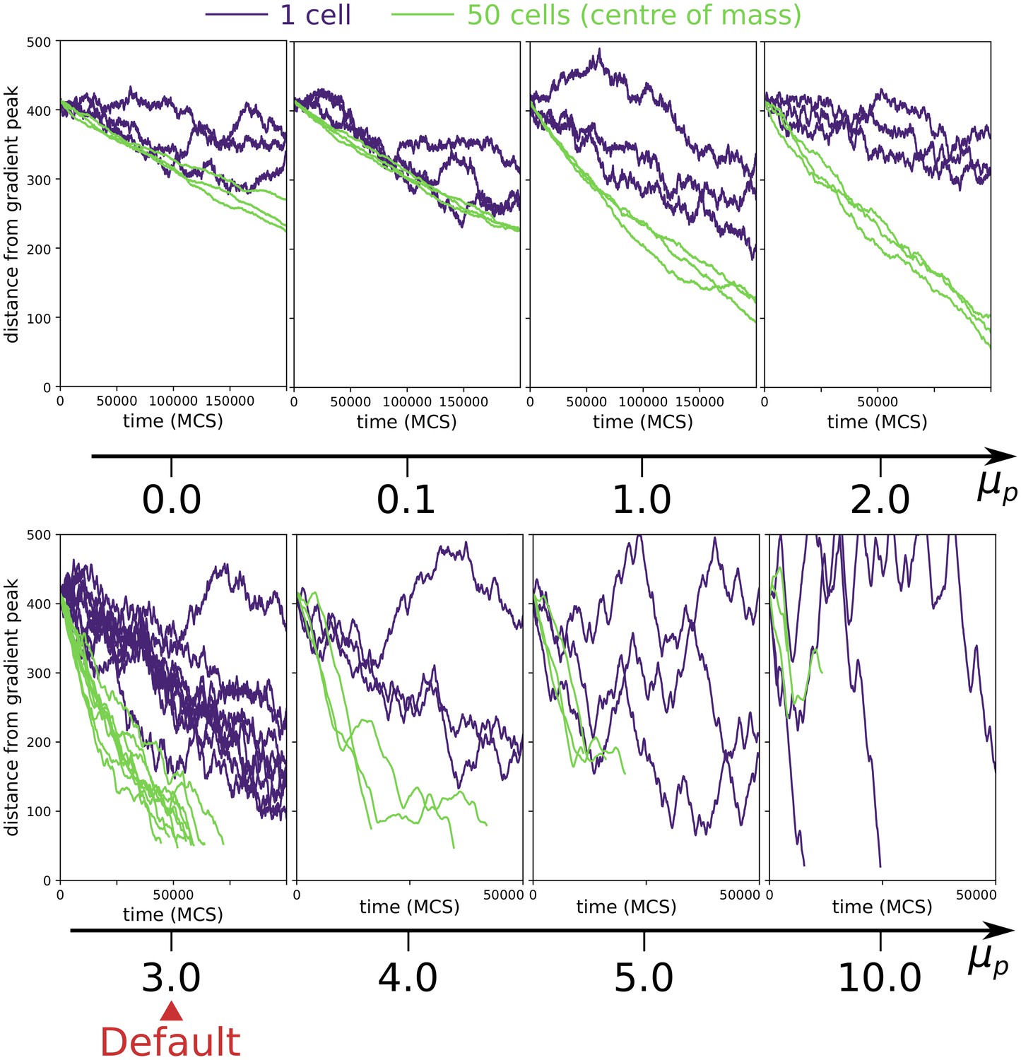
Collective vs. individual chemotaxis for different values of persistence strength $μ_{p} \in [0, 10]$ .

The plots show the displacement over time of the centre of mass of a single cell (indigo) and that of a cluster of 50 cells (green). Note that the x axis is different in different plots. The value of $μ_{p}$ used in main text is indicated by the Default sign. Three simulations are run for each parameter combination, except for the Default, where the same data of main text Figure 3a is shown. (All other parameters as in main text).

Appendix 1—figure 6

Download asset Open asset

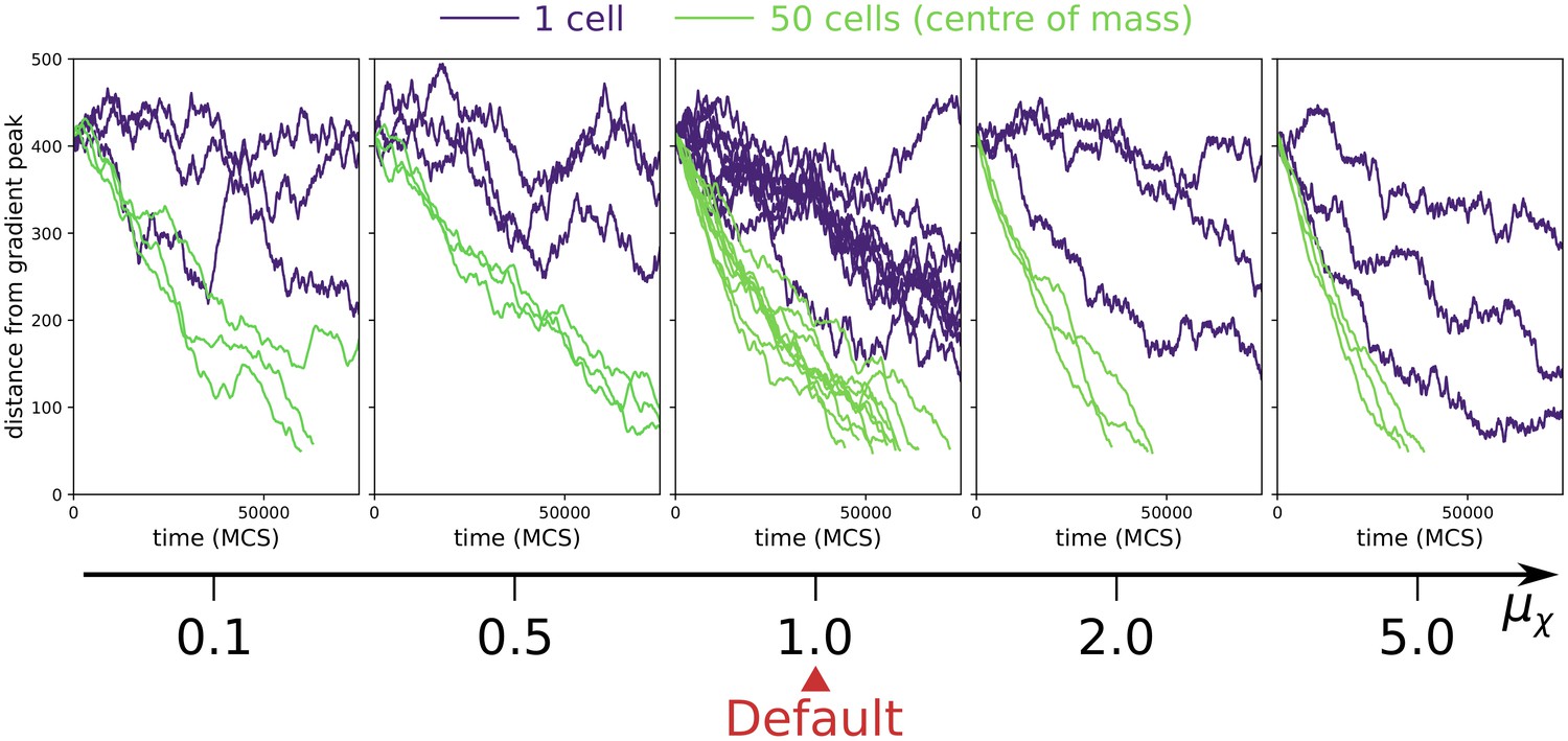
Collective vs. individual chemotaxis for different values of chemotactic strength $μ_{χ} \in [0.1, 5]$ .

The plots show the displacement over time of the centre of mass of a single cell (indigo) and that of a cluster of 50 cells (green). The value of $μ_{χ}$ used in main text is indicated by the Default sign. Three simulations are run for each parameter combination, except for the Default, where the same data of main text Figure 3a is shown. (All other parameters as in main text).

Appendix 1—figure 7

Download asset Open asset

Large cells perform chemotaxis more efficiently than clusters of small cells.

Each line corresponds to one simulation with a given combination of number of cells N and cell size $A_{T}$ , and shows the distance of the centre of mass of the cluster of cells from the peak of the gradient over time. We kept the total volume of the cells constant in all simulations (i.e. $N A_{T} = 5000$ ). All other parameters (including the chemotactic signal) are the same as in main text.

Appendix 1—figure 8

Download asset Open asset

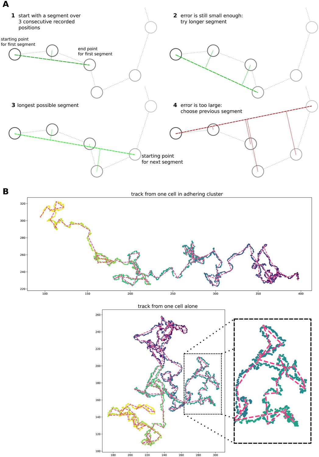
Simple algorithm for segment extraction.

(a) Visual explanation of the algorithm, with a cartoon representation of a cell track with cell positions recorded at regular time intervals. Images 1-4 represent subsequent stages of the algorithm. For 1–3, the maximum distance of intermediate cell positions is still small enough, while for the segment in image 4 two intermediate positions are too far away. So the segment in image 3 will be used in the analysis, and we will start the algorithm from the fourth data point. (b) Two cell tracks from simulations, with the extracted segments superimposed in red.

Appendix 2—figure 1

Download asset Open asset

Surface tension distribution for a population of cells that evolve adhesion, compared to the distribution of adhesion strength for randomly generated ligands and receptors.

The data for adhering cells are taken from the same simulation used for main text Figure 5a, over 10 seasons after reaching evolutionary steady state with $τ_{s} = 100^{3}$ MCS. Black: all vs. all surface tension distribution (all possible pairwise cell interaction energies tested); red: observed distribution. All parameters are as in main text Figure 5a. Blue: surface tension of random ligand receptors (10⁵ pairs were generated). AUE: Arbitrary Units of Energy (see Table 1).

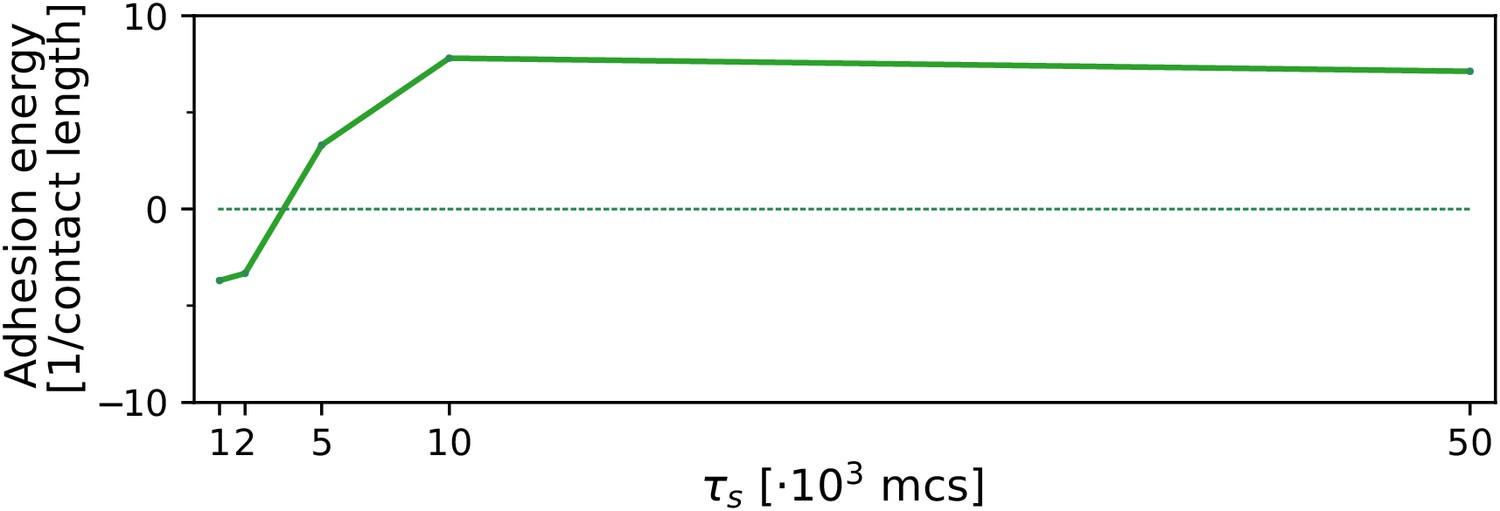
Appendix 2—figure 2

Download asset Open asset

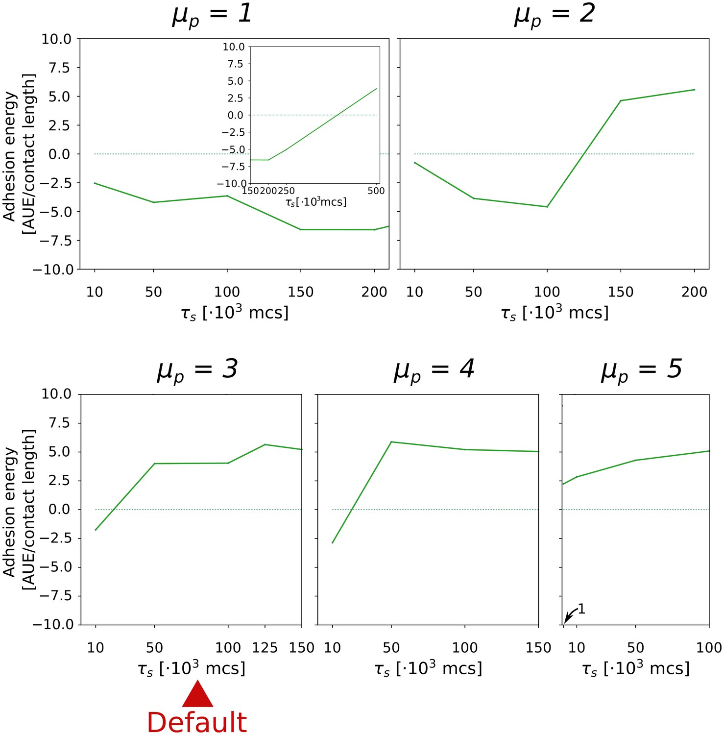
The evolution of multicellularity (and uni-cellularity) for different values of persistent migration strength $μ_{p} \in [1, 5]$ .

For $μ_{p} = 1$ , the inset shows the surface tension for $τ_{s} > 200 \times 10^{3}$ MCS. All other parameters and initialisation are as in main text Figure 5a.

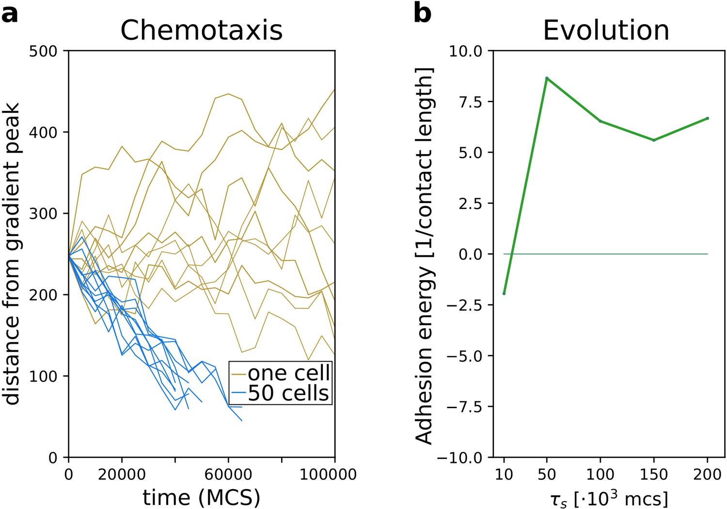
Appendix 2—figure 3

Download asset Open asset

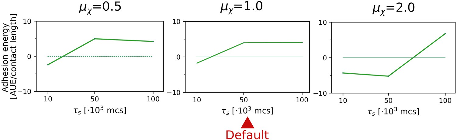
The evolution of multicellularity (and uni-cellularity) for different values of chemotactic strength $μ_{χ} \in [0.5, 2]$ .

All other parameters and initialisation are as in main text Figure 5a.

Appendix 2—figure 4

Download asset Open asset

The evolution of multicellularity (and uni-cellularity) when resources are spread for a chemoattractant gradient that decreases parallel from resources distributed on the entire side of the lattice.

All other parameters and initialisation are as in main text Figure 5.

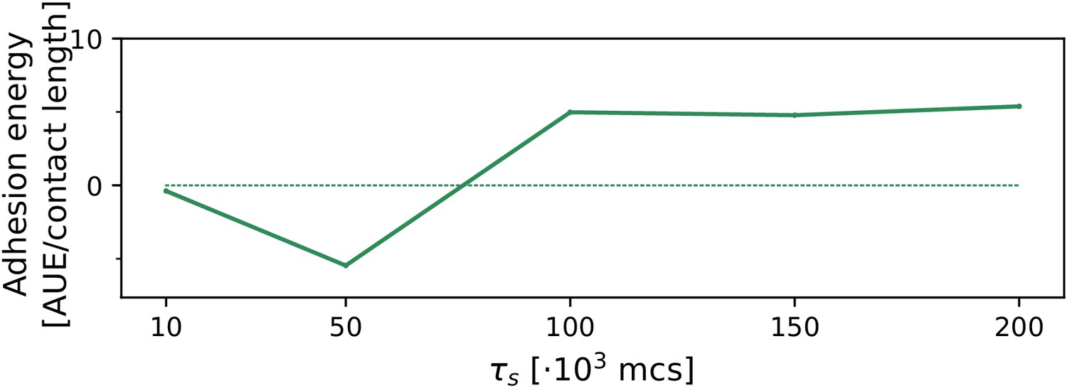
Appendix 2—figure 5

Download asset Open asset

The evolution of multicellularity (and uni-cellularity) with a steep, noiseless gradient ( $k_{χ} = 10$ , $p_{χ = 0} = 0$ ).

All other parameters and initialisation are as in main text Figure 5.

Appendix 3—figure 1

Download asset Open asset

Emergence of collective behaviour and evolution of multicellularity are robust to changing the mechanism of chemotaxis.

(a) The emergence of collective chemotaxis when individual cells cannot sense the gradient; (b) the evolution of multicellularity (and uni-cellularity) under these conditions. $μ_{CIL}$ - the strength of contact inhibition of locomotion is defined in the Materials and methods section. All other parameters and initialisation are as in main text Figure 5.

Appendix 4—figure 1

Download asset Open asset

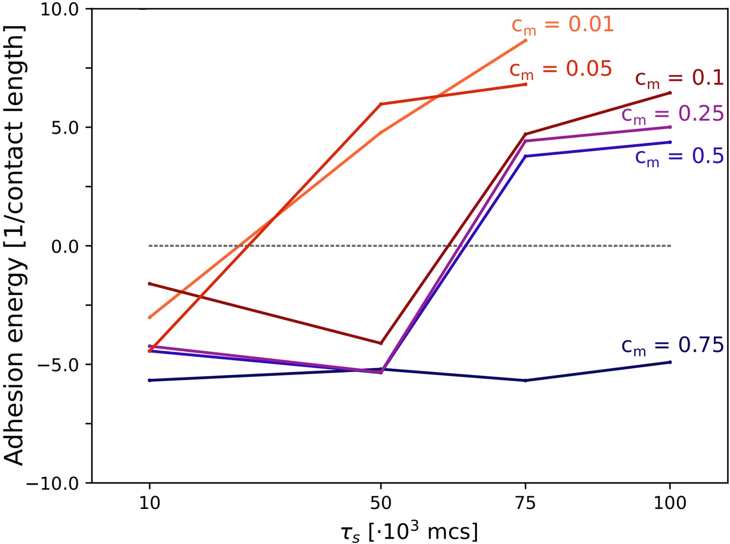
The evolution of multicellularity (and uni-cellularity) when adhesion is costly.

Different lines correspond to the evolutionary steady state at different season duration $τ_{s}$ for different values of costs c_m, as indicated in the figure. All other parameters and initialisation are as in main text Figure 5.

Videos

Video 1

Download asset

posterframe for video — Inefficient chemotaxis of a single cell.

Video 2

Download asset

Video 3

Download asset

Video 4

Download asset

Video 5

Download asset

Video 6

Download asset

Video 7

Download asset

Tables

Table 1

Parameters.

Parameter	Explanation	Values
$L^{2}$	lattice size	500 × 500 lattice sites
T	Boltzmann temperature	16 AUE
$λ$	cell stiffness	5.0 AUE/[lattice site]²
$A_{T}$	cell targetarea	50 lattice sites
Cell adhesion
$J_{α}$	minimum J value between cells	4 AUE/[lattice site length]
$J_{α}^{'}$	minimum J value between cell and medium	8 AUE/[lattice site length]
$ν$	length of receptor and ligand bitstring	24 bits
$ν^{'}$	length ligand bitstring for medium adhesion	six bits
Cell migration and chemotaxis
$μ_{p}$	strength of persistent migration	3.0 AUE
$τ_{p}$	duration of persistence vector	50 MCS
$μ_{χ}$	strength of chemotaxis	1.0 AUE
$k_{χ}$	scaling factor chemoattractant gradient	1.0 molecules/[lattice site length]
$p_{χ = 0}$	probability of zero value (’hole’) in gradient	0.1 [lattice site]⁻¹
Evolution
N	population size	200 cells
$τ_{s}$	duration of season	5 × 10³ - 150 × 10³ MCS
h_d	distance from gradient peak where fitness is $\frac{1}{2}$	50 [lattice site length]
$μ_{R, I}$	receptor and ligand mutation probability	0.01 per bit, per replication

AUE: Arbitrary Units of Energy (see Hamiltonian in Model Section); lattice site: unit of area; lattice site length: unit of distance; MCS: Monte Carlo Step (unit of time).

Additional files

Transparent reporting form: https://cdn.elifesciences.org/articles/56349/elife-56349-transrepform-v2.docx
Download elife-56349-transrepform-v2.docx

Download links

A two-part list of links to download the article, or parts of the article, in various formats.

Downloads (link to download the article as PDF)

Article PDF

Open citations (links to open the citations from this article in various online reference manager services)

Mendeley

Cite this article (links to download the citations from this article in formats compatible with various reference manager tools)

Enrico Sandro Colizzi
Renske MA Vroomans
Roeland MH Merks

(2020)

Evolution of multicellularity by collective integration of spatial information

eLife 9:e56349.

https://doi.org/10.7554/eLife.56349

Figures

Model description.

The eco-evolutionary setup of the model.

A group of cells performs chemotaxis efficiently in a noisy shallow gradient.

Indivdual cell trajectories are noisy, also within a cluster.

The evolution of multicellularity.

Interference competition between adhering and non-adhering cells explains evolutionary bistability.

Diffusion exponent approximation.

The speed of a cluster towards the peak of the gradient saturates with larger cluster sizes.

The flow field of a cluster of cells with and without gradient.

Chemotaxis of a rigid cluster.

Collective vs. individual chemotaxis for different values of persistence strength $μ_{p} \in [0, 10]$ .

Collective vs. individual chemotaxis for different values of chemotactic strength $μ_{χ} \in [0.1, 5]$ .

Large cells perform chemotaxis more efficiently than clusters of small cells.

Simple algorithm for segment extraction.

Surface tension distribution for a population of cells that evolve adhesion, compared to the distribution of adhesion strength for randomly generated ligands and receptors.

The evolution of multicellularity (and uni-cellularity) for different values of persistent migration strength $μ_{p} \in [1, 5]$ .

The evolution of multicellularity (and uni-cellularity) for different values of chemotactic strength $μ_{χ} \in [0.5, 2]$ .

The evolution of multicellularity (and uni-cellularity) when resources are spread for a chemoattractant gradient that decreases parallel from resources distributed on the entire side of the lattice.

The evolution of multicellularity (and uni-cellularity) with a steep, noiseless gradient ( $k_{χ} = 10$ , $p_{χ = 0} = 0$ ).

Emergence of collective behaviour and evolution of multicellularity are robust to changing the mechanism of chemotaxis.

The evolution of multicellularity (and uni-cellularity) when adhesion is costly.

Videos

Inefficient chemotaxis of a single cell.

Chemotaxis of a cluster of adhering cells.

Inefficient chemotaxis of a cluster of non-adhering cells.

The same cluster of adhering cells.

Video of an evolutionary simulation, starting with neutrally adhering cells ( $γ = 0$ ).

Over time a population of non-adhering cells spread throughout the lattice, when seasons are short.

Over time a population of adhering cells ends up in the centre of the lattice when seasons are short.

Tables

Parameters.

Additional files

Transparent reporting form

Download links

Downloads (link to download the article as PDF)

Open citations (links to open the citations from this article in various online reference manager services)

Cite this article (links to download the citations from this article in formats compatible with various reference manager tools)

Be the first to read new articles from eLife

Share this article

Cite this article

Model description.

The eco-evolutionary setup of the model.

A group of cells performs chemotaxis efficiently in a noisy shallow gradient.

Indivdual cell trajectories are noisy, also within a cluster.

The evolution of multicellularity.

Interference competition between adhering and non-adhering cells explains evolutionary bistability.

Diffusion exponent approximation.

The speed of a cluster towards the peak of the gradient saturates with larger cluster sizes.

The flow field of a cluster of cells with and without gradient.

Chemotaxis of a rigid cluster.

Collective vs. individual chemotaxis for different values of persistence strength μp∈[0,10].

Collective vs. individual chemotaxis for different values of chemotactic strength μχ∈[0.1,5].

Large cells perform chemotaxis more efficiently than clusters of small cells.

Simple algorithm for segment extraction.

Surface tension distribution for a population of cells that evolve adhesion, compared to the distribution of adhesion strength for randomly generated ligands and receptors.

The evolution of multicellularity (and uni-cellularity) for different values of persistent migration strength μp∈[1,5].

The evolution of multicellularity (and uni-cellularity) for different values of chemotactic strength μχ∈[0.5,2].

The evolution of multicellularity (and uni-cellularity) when resources are spread for a chemoattractant gradient that decreases parallel from resources distributed on the entire side of the lattice.

The evolution of multicellularity (and uni-cellularity) with a steep, noiseless gradient (kχ=10, pχ=0=0).

Emergence of collective behaviour and evolution of multicellularity are robust to changing the mechanism of chemotaxis.

The evolution of multicellularity (and uni-cellularity) when adhesion is costly.

Inefficient chemotaxis of a single cell.

Chemotaxis of a cluster of adhering cells.

Inefficient chemotaxis of a cluster of non-adhering cells.

The same cluster of adhering cells.

Video of an evolutionary simulation, starting with neutrally adhering cells (γ=0).

Over time a population of non-adhering cells spread throughout the lattice, when seasons are short.

Over time a population of adhering cells ends up in the centre of the lattice when seasons are short.

Parameters.

Transparent reporting form

Downloads (link to download the article as PDF)

Open citations (links to open the citations from this article in various online reference manager services)

Cite this article (links to download the citations from this article in formats compatible with various reference manager tools)

Collective vs. individual chemotaxis for different values of persistence strength $μ_{p} \in [0, 10]$ .

Collective vs. individual chemotaxis for different values of chemotactic strength $μ_{χ} \in [0.1, 5]$ .

The evolution of multicellularity (and uni-cellularity) for different values of persistent migration strength $μ_{p} \in [1, 5]$ .

The evolution of multicellularity (and uni-cellularity) for different values of chemotactic strength $μ_{χ} \in [0.5, 2]$ .

The evolution of multicellularity (and uni-cellularity) with a steep, noiseless gradient ( $k_{χ} = 10$ , $p_{χ = 0} = 0$ ).

Video of an evolutionary simulation, starting with neutrally adhering cells ( $γ = 0$ ).