High-fidelity musculoskeletal modeling reveals that motor planning variability contributes to the speed-accuracy tradeoff
Figures
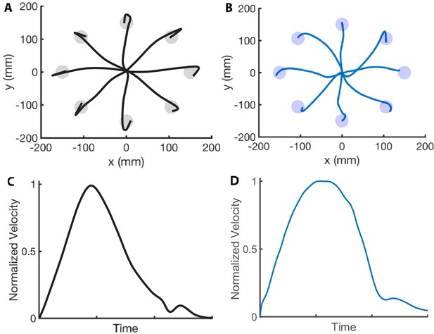
Center-out reaching.
(A and B) Hand paths adapted from Beer et al., 2000 (A) compared to hand paths produced by our computational model (B) during a center-out fast reaching task with targets placed 150 mm away from the center position. (C and D) Mean velocity profile in a reaching task adapted from Soechting, 1984 (C) compared to the velocity profile produced by our computational model (D). We reproduce the bell-shaped velocity profile, including the smaller velocity peak at the end of the movement.

Velocity profile based on target size and speed.
(A) Effect of the target size in reaching movements. The dashed curve is the average velocity profile for the larger target, while the solid curve is for the smallest target (adapted from Soechting, 1984). (B) Average velocity profile of 15 runs from our simulations to a small and large target. All the curves are normalized to their peak velocity. (C) Normalized velocity profiles (with normalized time) for fast, medium, and slow movements. Our results are consistent with the observation (e.g., Nagasaki, 1989) that slower movements tend to have an earlier peak velocity than faster movements.
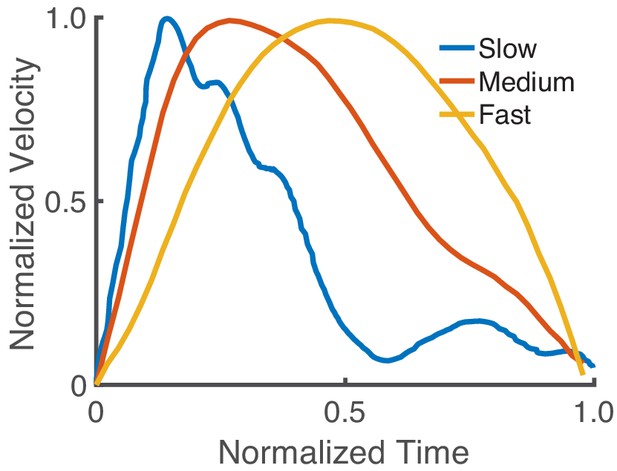
Asymmetry of the velocity profile based on speed with a realistic biomechanical model.
Normalized velocity profiles (with normalized time) for fast (0.15 s movement duration [MD]), medium (0.25 s MD), and slow movements (0.45 s MD). Our model reproduces the speed-dependent asymmetry in the velocity profile. The relative peak velocities are 0.6133, 0.41, and 0.19 for the fast, medium, and slow movements, respectively.
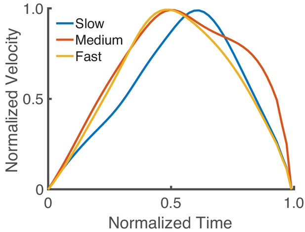
Asymmetry of the velocity profile based on speed with a torque-driven model.
Normalized velocity profiles (with normalized time) for fast, medium, and slow movements (15 s, 20 s, and 25 s movement durations, respectively). The torque-driven model does not reproduce the observation that faster movements tend to have a later peak velocity than slower movements, while this was reproduced with our realistic muscle-based model (see Figure 2C).
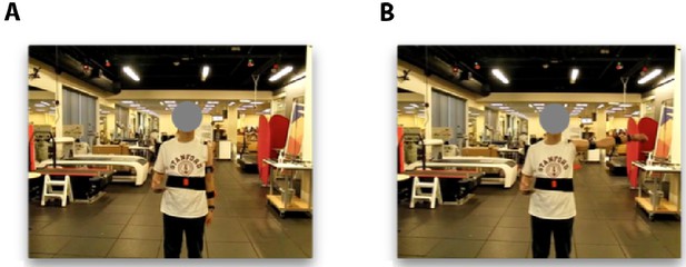
Data collection.
(A and B) Subjects are asked to move to a desired final pose (B) from a given initial pose (A). This figure is an example of a shoulder 0−90° abduction movement.
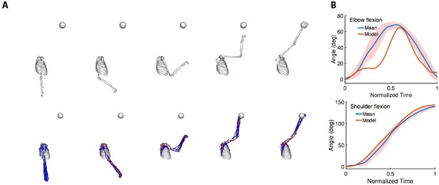
Movement comparison.
(A) We compare the reaches to a target (the sphere) of a representative subject (top; model without muscles) with the reaches synthesized by our computational model (bottom; model with muscles). (B) Joint kinematics. We plot the sagittal joint angles in the reaching movement. We compare the elbow and shoulder flexion angles over time from our model and the means from experiments. The shaded region is one standard deviation from the mean.

Speed-accuracy tradeoff.
(A) Movement duration (MD) depending on the index of difficulty from the dataset in Goldberg et al., 2014. The mean and standard deviation are computed from 334 trials and 46 subjects (statistics computed across subjects). The experiment consists in subjects reaching with a mouse to targets of various distances and widths on a computer screen. (B) MD depending on the index of difficulty for a representative subject from Goldberg et al., 2014 with statistics computed from seven trials to each target. (C) Predicted MD to a target in a center-out reaching task when varying the target size. The x-axis is the index of difficulty of the reaching movement, which varies from 0.9 (width: 0.16 m) to 4.41 (width: 0.014 m). The vertical bars are one standard deviation from the mean. We see that the model’s mean predictions are in close agreement with Fitts’ law (R2 = 0.974).

Speed-accuracy tradeoff with a torque-driven model.
Predicted movement duration (MD) to a target in a reaching task when varying the target size with our torque-driven model. The x-axis is the index of difficulty of the reaching movement, which varies from 0.9 (width: 0.16 m) to 3.9 (width: 0.02 m). The vertical bars are one standard deviation from the mean. We see that the model’s mean predictions are in close agreement with Fitts’ law (R2 = 0.88). Qualitatively, we see that unlike our muscle-based model (see Figure 3C), the results with the torque-driven model do not clearly predict the increase in MD variance with more severe task constraints. Both the predicted means and standard deviations are not statistically correlated with the experimental data in Figure 3A.
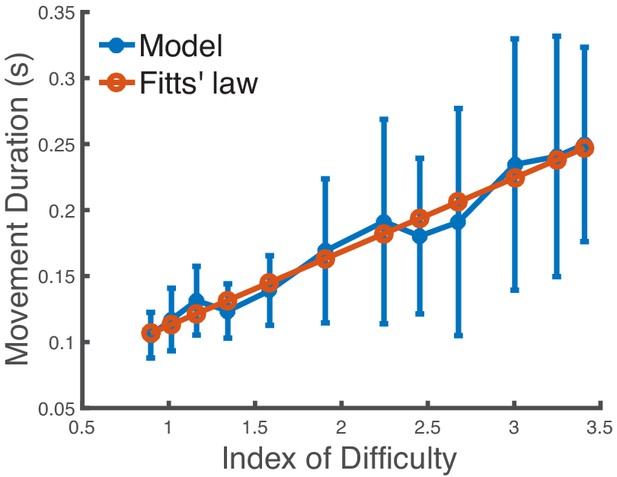
Impact of the optimizer on the speed-accuracy tradeoff.
We use a much less effective trajectory optimizer than in Figure 3C to predict the movement duration to a target in a center-out reaching task when varying the target size. The x-axis is the index of difficulty of the reaching movement. We see that the model’s mean predictions are still in very close agreement with Fitts’ law (R2 = 0.969).
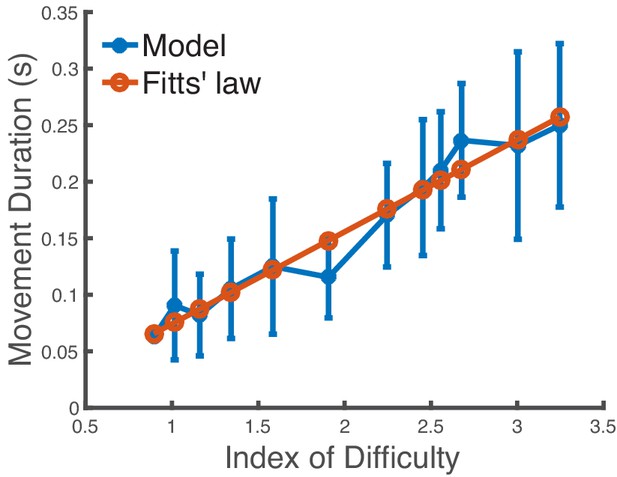
Impact of the muscle activations term on the speed-accuracy tradeoff.
Predicted movement duration to a target in a reaching task when varying the target size without the muscle activation term in Equation 1. The x-axis is the index of difficulty of the reaching movement. We use covariance matrix adaptation evolution strategy with 20 iterations and 20 samples to generate the trajectories. We see that the model’s mean predictions are still in close agreement with Fitts’ law (R2 = 0.955), which indicates that the muscle activations term alone is not sufficient to explain the speed-accuracy tradeoff. The standard deviations are not statistically correlated with the experimental data in Figure 3A. The vertical bars are one standard deviation from the mean.

Impact of the force–length relationship in muscles.
Predicted movement duration to a target in a reaching task when using a simplified biomechanical model with muscles having a constant active force-length relationship (instead of a bell-shaped curve as described in Millard et al., 2013). The x-axis is the index of difficulty of the reaching movement. We see that the model’s mean predictions are in agreement with Fitts’ law (R2 = 0.94). The standard deviations are not statistically correlated with the experimental data in Figure 3A. The vertical bars are one standard deviation from the mean.
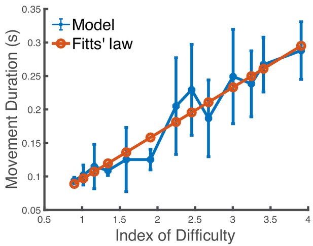
Impact of a simplified model with fewer muscles.
Predicted movement duration to a target in a reaching task when varying the target size when we use a model with 14 important muscles missing (deltoid anterior, deltoid posterior, infraspinatus, teres minor, etc.). The x-axis is the index of difficulty of the reaching movement. We use covariance matrix adaptation evolution strategy with 20 iterations and 20 samples to generate the trajectories. We see that the model’s mean predictions are in close agreement with Fitts’ law (R2 = 0.93). The standard deviations are not statistically correlated with the experimental data in Figure 3A. The vertical bars are one standard deviation from the mean.

Simulated hand paths.
Ten simulated hand paths when reaching for a large and small target 15 cm in distance. In this example, the average movement durations are 0.15 s and 0.22 s, respectively. The simulated muscle activity and kinematics are provided in supplementary material.
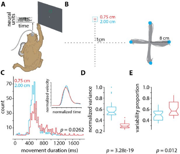
Neural data and analysis.
(A) Rhesus monkey reaches in 3D space using his right arm, while neural activity from 192 channels are recorded from two Utah arrays surgically implanted into contralateral dorsal premotor and primary motor cortex. The monkey’s arm position in space controlled the velocity of the cursor on the screen (methods described in Even-Chen et al., 2019). (B) (Left) the layout of the 40 targets to which the monkey reaches. For each of the 40 targets, two conditions are presented in a block-wise format. In one condition (block) the target has an acceptance window of size 2 cm (cyan), and in the other the acceptance window is of size 0.75 cm (red). Within each block, the targets appear randomly. Each block contains 400 trials (10 trials per target), and each experimental session contains about 10 blocks, 5 of each condition. (Right) representative arm reaches made by the monkey for four targets 8 cm away from the center with an acceptance window size of 2 cm. (C) Histograms of movement duration (MD) for the large (2 cm) and small (0.75 cm) targets (inset shows the normalized velocity profiles). The observed difference in variance is statistically significant (p=0.0262 via two-sample F-test). The MDs to the large and small targets are 461 ± 234 ms and 661 ± 258 ms. (D) Normalized variance of the preparatory neural state for the small (0.75 cm targets, red) and large (2.00 cm targets, cyan) targets. The variance in the preparatory state is computed by first taking trial-averaged firing rates for the last 200 ms of preparation before the go-cue, performing principal components analysis, and finding the volume of the error ellipse in 3D space, which captures at least 80% of the total variance (similar to as described in Vyas et al., 2018 and Even-Chen et al., 2019). Note that we do not spike sort or assign spikes to individual neurons (Wood et al., 2004). We instead use threshold crossings (Trautmann et al., 2019). (E) Proportion of movement variability explained by preparatory variability (as described in Churchland et al., 2006a), for the small (0.75 cm targets, red) and large (2.00 cm targets, cyan) targets. In D and E the p-values are computed from one-way ANOVA.
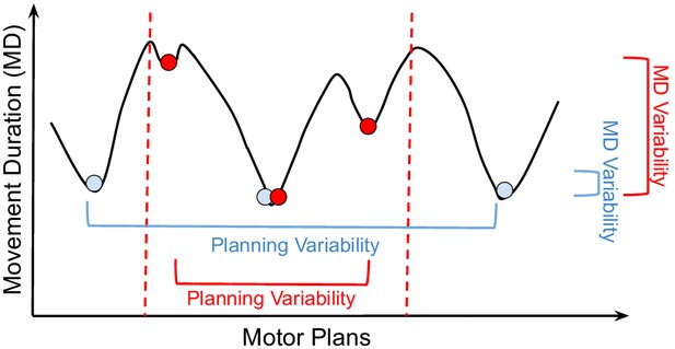
Optimization landscape.
Cartoon of how different motor plans can generate movements (i.e., driven by muscle excitation patterns) with different durations. The blue and red circles are examples of control solutions for the large and small targets, respectively. The dashed lines illustrate the constraints in the optimization landscape for the smaller target. From the analysis in Figure 4C and D, for reaches to a small target (red), movement planning variability decreases (x-axis), but movement duration (MD) variability increases (y-axis). For reaches to a larger target (blue), movement planning variability increases, but MD variability decreases. According to our theory, reaches to larger targets are faster because of the presence of good control solutions in the optimization landscape. We empirically observe that these good solutions have MDs that are only slightly larger than the global minimum solution (i.e., the fastest reach to the target). A bad control solution corresponds to a significantly slower reach. On average, reaches to the small target are slower because tighter constraints remove good solutions from the optimization landscape, which is otherwise identical to the landscape for the large target. While this decreases motor planning variability, it increases MD variability. In stochastic optimization, it is empirically found that having a large number of good local minima helps avoid bad local minima (Goodfellow et al., 2016, Chapter 8).
Videos
Comparison of reaching movements between a representative subject (model without muscles) and our computational model (model with muscles).
Tables
Impact of the biomechanical model.
We summarize how our results vary based on the biomechanical model. We tested six different models: a torque-driven model, a musculoskeletal model missing 14 important muscles (e.g., deltoid anterior, deltoid posterior, infraspinatus, teres minor, etc.), a musculoskeletal model with unrealistic muscle force–length relationships, a musculoskeletal model with an unrealistic cost function, a realistic musculoskeletal model with an effective optimizer, and a realistic musculoskeletal with a less effective optimizer. The results for the model ‘without planning variability’ are taken from the literature.
| Fitts’ law | Behavior results correlated with experimental data (MD means and standard deviations) | |
|---|---|---|
| Torque or musculoskeletal model with signal-dependent noise and without planning variability | Yes | No |
| Torque model | Yes | No |
| Musculoskeletal model with missing muscles | Yes | No |
| Musculoskeletal model with unrealistic force–length relationships | Yes | No |
| Musculoskeletal model with an unrealistic cost function (i.e., no muscle activations term) | Yes | No |
| Musculoskeletal model with an effective optimizer | Yes | Yes |
| Musculoskeletal model with a less effective optimizer | Yes | Yes |
Model Parameters.
| Fitts’ Law | Behavior Results Correlated with Experimental Data (movement duration means and standard deviations) | |
|---|---|---|
| Torque or Musculoskeletal Model with Signal-Dependent Noise and without Planning Variability | Yes | No |
| Torque Model with Planning Variability | Yes | No |
| Musculoskeletal Model with Planning Variability | Yes | Yes |
Impact of the Biomechanical Model.
We summarize how our results vary based on the biomechanical model. We tested six different models: a torque-driven model, a musculoskeletal model missing 14 important muscles (e.g., deltoid anterior, deltoid posterior, infraspinatus, teres minor, etc.), a musculoskeletal model with unrealistic muscle force-length relationships, a musculoskeletal model with an unrealistic cost function, a realistic musculoskeletal model with an effective optimizer, and a realistic musculoskeletal with a less effective optimizer. The results for the model “without planning variability” are taken from the literature.
| Fitts’ Law | Behavior Results Correlated with Experimental Data (movement duration means and standard deviations) | |
|---|---|---|
| Torque or musculoskeletal model with signal-dependent noise and without planning variability | Yes | No |
| Torque model | Yes | No |
| Musculoskeletal model with missing muscles | Yes | No |
| Musculoskeletal model with unrealistic force-length relationships | Yes | No |
| Musculoskeletal model with an unrealistic cost function (i.e., no muscle activations term) | Yes | No |
| Musculoskeletal model with an effective optimizer | Yes | Yes |
| Musculoskeletal model with a less effective optimizer | Yes | Yes |
Additional files
-
Supplementary file 1
Fast reaching experimental data.
For five subjects, we present the mean, standard deviation, minimum, and maximum of the movement durations in 10 reaches to a large (L) and small (S) square targets (see the section Fast reaching task). The target widths are 8 cm and 2 cm, and the reach amplitudes are 15 cm. The data are available at https://simtk.org/projects/ue-reaching/.
- https://cdn.elifesciences.org/articles/57021/elife-57021-supp1-v2.docx
-
Transparent reporting form
- https://cdn.elifesciences.org/articles/57021/elife-57021-transrepform-v2.docx


