Epithelial colonies in vitro elongate through collective effects
- Laboratory of Cell Physics ISIS/IGBMC, CNRS and Université de Strasbourg, France
- Institut de Génétique et de Biologie Moléculaire et Cellulaire, France
- Centre National de la Recherche Scientifique, UMR7104, France
- Institut National de la Santé et de la Recherche Médicale, U964, France
- Department of Civil Engineering, Indian Institute of Technology Bombay, Powai, India
- Department of Mechanical Engineering, Indian Institute of Technology Bombay, Powai, India
- The Francis Crick Institute, United Kingdom
- Max Planck Institute for the Physics of Complex Systems, Germany
- Cluster of Excellence Physics of Life, Germany
Figures
Figure 1 with 2 supplements
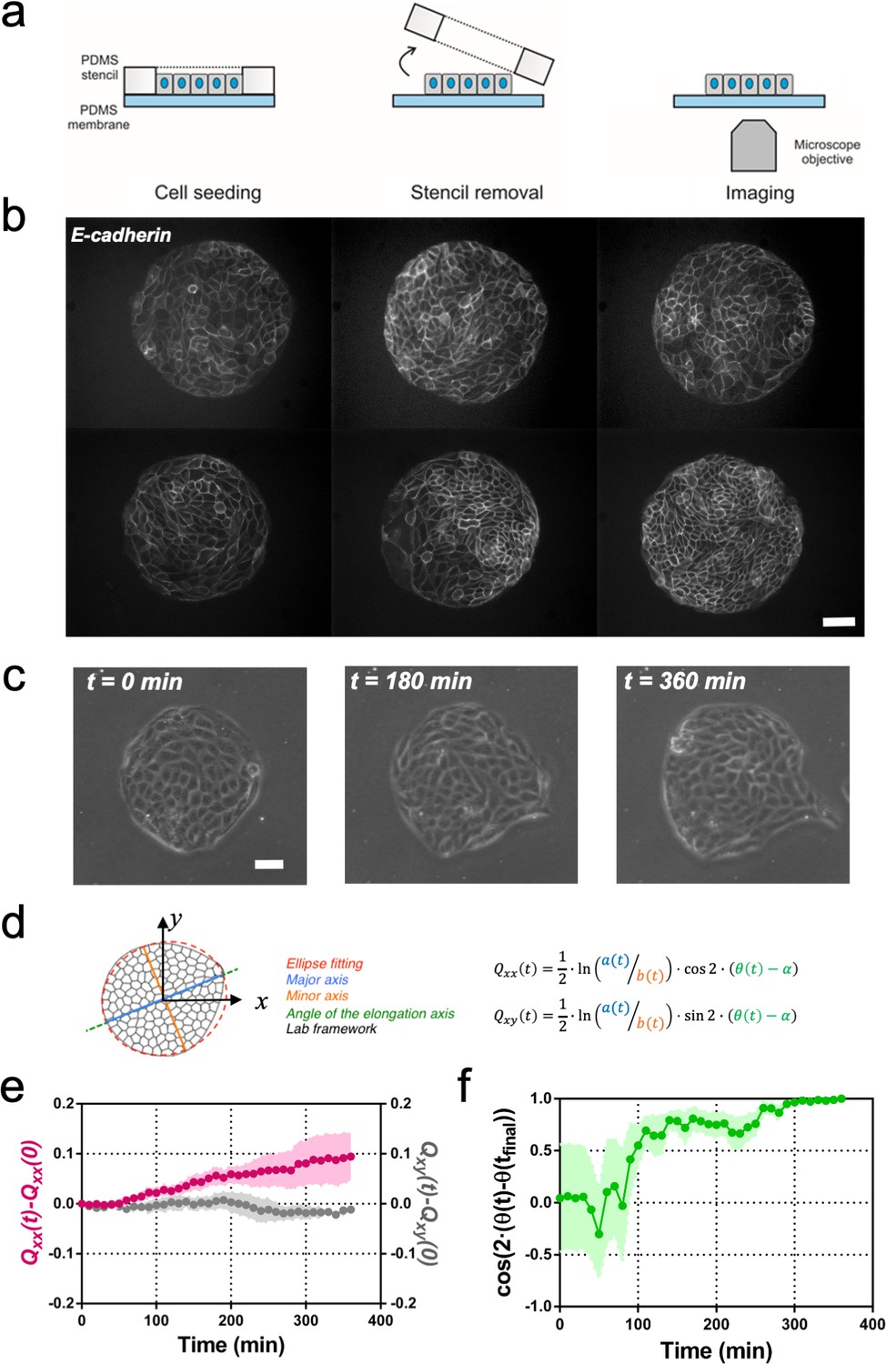
Symmetry breaking and its quantification.
(a) Schematics of the experimental set-up: Madin Darby Canine Kidney (MDCK) cells were seeded on a poly(dimethylsiloxane) (PDMS) membrane using stencils to predefine their shape. When the colony was confluent, the stencil was removed and the expansion of the colony was observed under the microscope. (b) Several examples of MDCK colonies (GFP-E-cadherin) after stencil removal and prior to colony expansion. Scale bar 50 µm. (c) Phase contrast images of the spontaneous elongation of an MDCK colony for 360 min. Scale bar 50 µm. (d) Colony elongation is quantified by ellipse fitting and Qxx and Qxy measurement referred to the elongation axis (α = θ(tfinal)). (e) Qxx (left y axis) and Qxy (right y axis) during 360 min of colony expansion. Mean value ± standard error of the mean, n = 4 colonies from N = 4 independent experiments. (f) Cosine of two times the angle difference between the instantaneous main direction of the colony (θ(t)) and the main direction of the colony at 360 min (θ(tfinal)). Colonies set the elongation direction within the first 120 min. Mean value ± standard error of the mean, n = 4 colonies from N = 4 independent experiments.
-
Figure 1—source data 1
The Qxx(t)-Qxx(0) and Qxy(t)-Qxy(0) of individual colonies used in panel (e) and the raw values of cos(2·(θ(t)-θ(tfinal))) used in panel (f) of Figure 1.
- https://cdn.elifesciences.org/articles/57730/elife-57730-fig1-data1-v2.xlsx
Figure 1—figure supplement 1
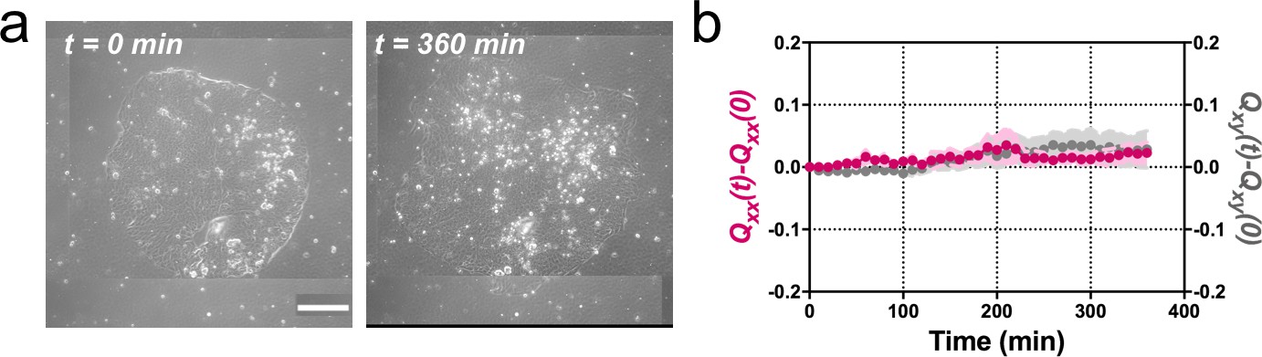
Madin Darby Canine Kidney (MDCK) colonies of 750 µm in diameter expand isotropically.
(a) Phase contrast images of the spontaneous expansion of an MDCK colony for 360 min. Scale bar 200 µm. (b) Qxx (left y axis) and Qxy (right y axis) during 360 min of colony expansion. Mean value ± standard error of the mean, n = 3 colonies from N = 3 independent experiments.
-
Figure 1—figure supplement 1—source data 1
Qxx(t)-Qxx(0) and Qxy(t)-Qxy(0) for the three 750 µm in diameter individual colonies of MDCK cells expanding for 6 hours.
- https://cdn.elifesciences.org/articles/57730/elife-57730-fig1-figsupp1-data1-v2.xlsx
Figure 1—figure supplement 2
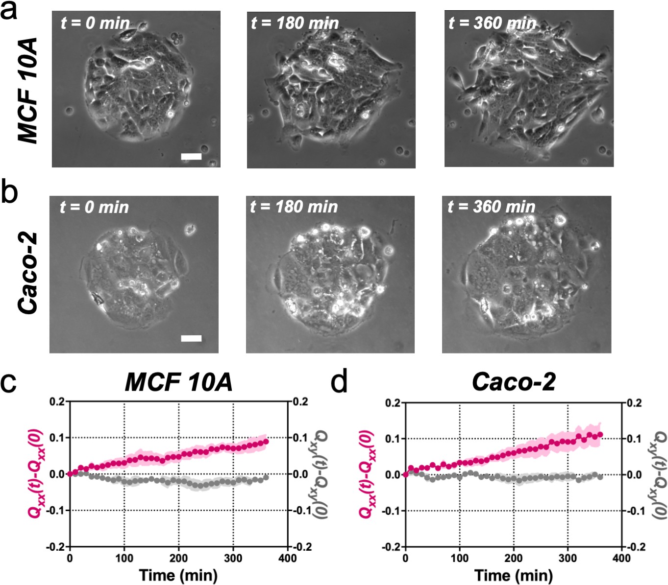
MCF 10A and Caco-2 colonies of 250 µm in diameter expand asymmetrically similar to Madin Darby Canine Kidney (MDCK) colonies.
(a) Phase-contrast images of the spontaneous elongation of an MCF (Michigan Cancer Foundation) 10A colony for 360 min. Scale bar 50 µm. (b) Phase-contrast images of the spontaneous elongation of a Caco-2 colony for 360 min. Scale bar 50 µm. (c) Qxx (left y axis) and Qxy (right y axis) during 360 min of MCF 1A colony expansion. Mean value ± standard error of the mean, n = 10 colonies from N = 3 independent experiments. (d) Qxx (left y axis) and Qxy (right y axis) during 360 min of Caco-2 colony expansion. Mean value ± standard error of the mean, n = 6 colonies from N = 3 independent experiments.
-
Figure 1—figure supplement 2—source data 1
Raw data corresponding to panels (c) and (d): Qxx(t)-Qxx(0) and Qxy(t)-Qxy(0) for individual colonies (250 µm in diameter) of MCF 10A cells and Caco-2 expanding for 6 hours.
- https://cdn.elifesciences.org/articles/57730/elife-57730-fig1-figsupp2-data1-v2.xlsx
Figure 2 with 1 supplement
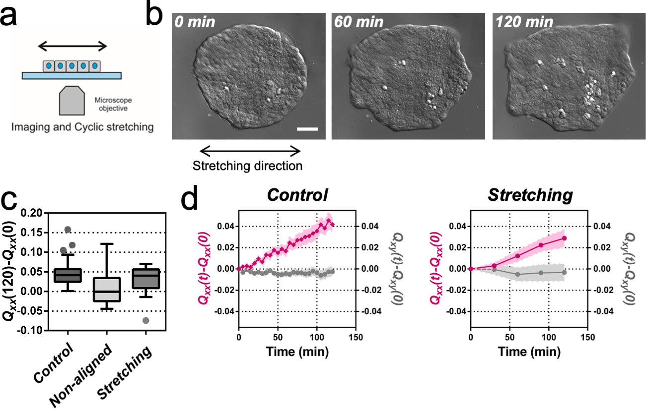
Uniaxial cyclic stretching rectifies symmetry breaking.
(a) Schematics of the experiment where the colony expansion was observed under the microscope while the underlying membrane was uniaxially stretched. (b) Snapshots of the expansion of a Madin Darby Canine Kidney (MDCK) colony while cyclically stretched. Scale bar 50 µm. (c) Colony elongation (Qxx) of control colonies along the elongation axis, control colonies in the laboratory framework (non-aligned, α = 0) and colonies under cyclic uniaxial stretching in the laboratory framework (uniaxial stretching, α = 0). Box Plot between 25th and 75th percentile, being the line in the box the median value, whiskers and outliers (dots) are obtained following Tukey’s method, Ncontrol = 11 independent experiments, n = 25 colonies and Nstretching = 9, n = 20 colonies. Mann-Whitney test control vs control aligned p=0.0003, control vs stretching p=0.0281 and control aligned vs stretching p=0.3319. (d) Qxx (left y axis) and Qxy (right y axis) during 120 min of colony expansion for control colonies and colonies under cyclic uniaxial stretching. Mean value ± standard error of the mean, Ncontrol = 8, n > 14 colonies and Nstretching = 9, n = 20 colonies.
-
Figure 2—source data 1
Raw data used for the panel (c) of Figure 2 and Qxx(t)-Qxx(0) and Qxy(t)-Qxy(0) for the individual colonies used for panel (d) of Figure 2.
- https://cdn.elifesciences.org/articles/57730/elife-57730-fig2-data1-v2.xlsx
Figure 2—figure supplement 1
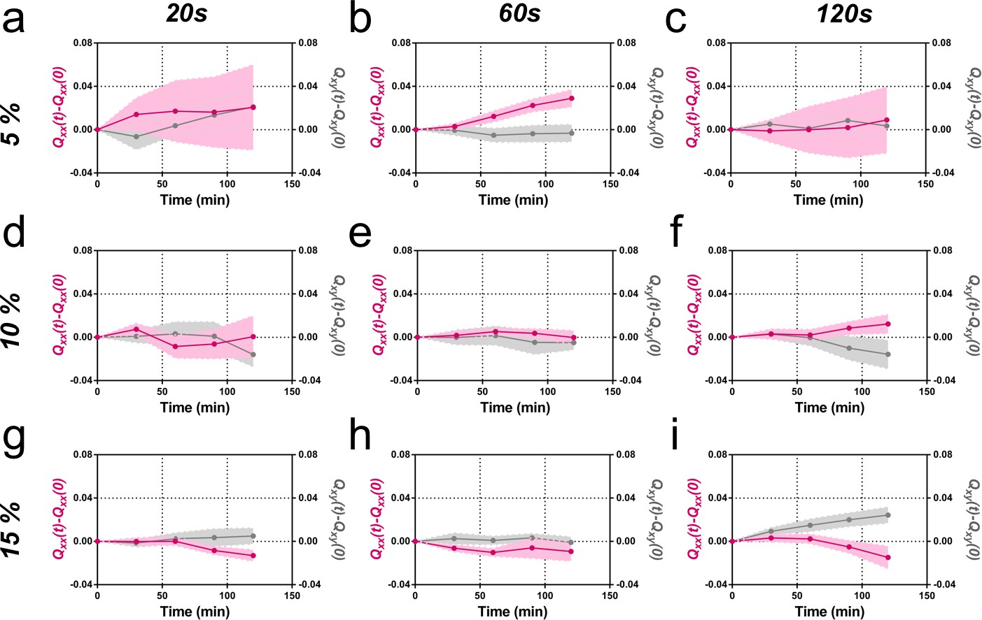
Elongation as a function of frequency and amplitude of cyclic uniaxial stretching.
Cumulative Qxx (left y axis) and cumulative Qxy (right y axis) during 120 min of colony expansion (α = 0). Mean value ± standard error of the mean. (a) Five percent amplitude and 20 s frequency N = 3, n = 5 colonies. (b) Five percent amplitude and 60 s frequency N = 9, n = 20 colonies. (c) Five percent amplitude and 120 s frequency N = 5, n = 6 colonies. (d) Ten percent amplitude and 20 s frequency N = 4, n = 6 colonies. (e) Ten percent amplitude and 60 s frequency N = 5, n = 8 colonies. (f) Ten percent amplitude and 120 s frequency N = 4, n = 8 colonies. (g) Fifteen percent amplitude and 20 s frequency N = 3, n = 9 colonies. (h) Fifteen percent amplitude and 60 s frequency N = 3, n = 6 colonies. (i) Fifteen percent amplitude and 120 s frequency N = 3, n = 6 colonies.
-
Figure 2—figure supplement 1—source data 1
Values of Qxx(t)-Qxx(0) and Qxy(t)-Qxy(0) for each of the colonies included in Figure 2—figure supplement 1.
- https://cdn.elifesciences.org/articles/57730/elife-57730-fig2-figsupp1-data1-v2.xlsx
Figure 3
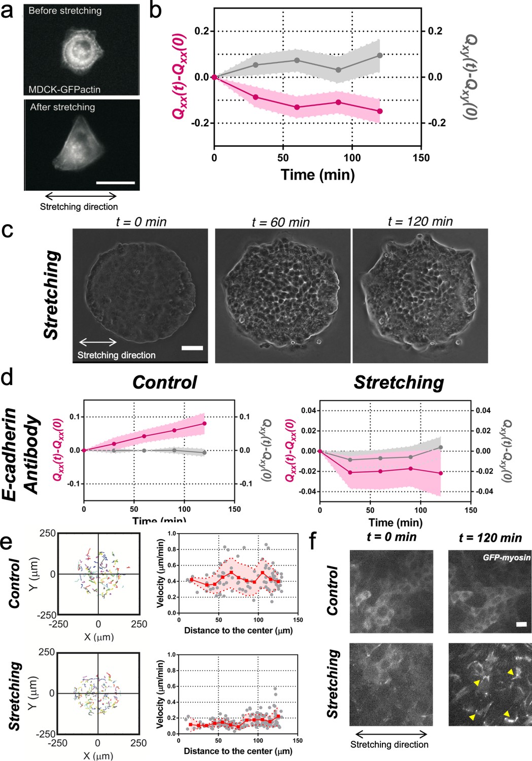
Collective effects are essential for rectification.
(a) Image of a single MDCK-GFP-actin cell before and after being stretch for 2 hr (5% strain and 60 s period). Scale bar 20 µm. (b) Qxx (left y axis) and Qxy (right y axis) of single cells during 120 min of cyclic uniaxial stretching (α = 0). Mean value ± standard error of the mean. N = 3, n = 31 cells. (c) Phase-contrast images of a Madin Darby Canine Kidney (MDCK) colony evolving for 120 min under cyclic mechanical stretching when E-cadherins are blocked by an E-cadherin antibody. Scale bar 50 µm. (d) Comparison of the cumulative Qxx (left y axis) and cumulative Qxy (right y axis) during 120 min of colony expansion when E-cadherin are blocked by an E-cadherin antibody in control and under cyclic uniaxial stretching (α = 0). Mean value ± standard error of the mean, Ncontrol = 3, n = 8 colonies and Nstretching = 4, n = 15 colonies. (e) Trajectories of cells (left) and single-cell velocity as a function of its distance to the center of the colony (right) in control colonies (top) and under cyclic uniaxial stretching (bottom). ncontrol = 90 cells from 8 colonies of Ncontrol = 4 independent experiments and nstretching = 154 cells from 13 colonies of Nstretching = 4 independent experiments. Individual cells in gray, red square and line corresponds mean (binned by distance to the center), shadowed area corresponds to SD. (f) Myosin distribution inside MDCK-GFP-myosin colonies at 0 min and at 120 min after expansion in control and under uniaxial stretching. Note the myosin structures appearing in the stretching case (yellow arrows). Scale bar 10 µm.
-
Figure 3—source data 1
The Qxx(t)-Qxx(0) and Qxy(t)-Qxy(0) of individual cells used in panel (b) and individual colonies used in panel (d); we also provide datasets for the velocities of individual cells in panel (e).
- https://cdn.elifesciences.org/articles/57730/elife-57730-fig3-data1-v2.xlsx
Figure 4 with 2 supplements
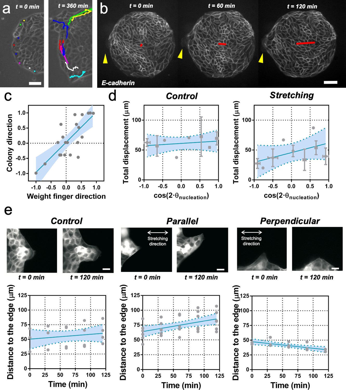
Fingers and symmetry breaking.
(a) Trajectories of boundary cells during colony expansion. Two types of trajectories are observed: radial and tangential. Scale bar 50 µm. (b) Fluorescent images (GFP-E-cadherin) of a colony evolving for 120 min. Red line shows the orientation of the colony according to ellipse fitting (length scales with the change in Qxx) and yellow arrow indicates a cell migrating radially. Scale bar 50 µm. (c) Direction of the colony elongation (quantified by the cosine of two times the angle of the main axis of the colony at t = 2 hr) as a function of the weight finger direction (quantified by the average of the cosine of two times the angle of each finger trajectory, for example the angle corresponding to the vector between the position of the finger at t = 0 hr and t = 2 hr, of each finger weight by the finger’s displacement). N = 5, ncolonies = 12 colonies and nfinger = 21 fingers. Blue line corresponds to the linear fitting of the data points and the shadowed area corresponds to the 95% confidence interval. Pearson’s correlation coefficient r = 0.7724, p=0.0001. (d) Total displacement of finger growth as a function of its initial position in the colony (angular coordinate from the center of the colony) for control colonies and colonies under uniaxial stretching. N = 5 independent experiments, ncolonies = 11 colonies and nfinger = 21 fingers (control) and N = 6, ncolonies = 10 colonies and nfinger = 28 fingers (stretching). Averaged fingers in gray (both position and distance, Mean ± SD), blue line corresponds to the linear fitting of the data points and the shadowed area corresponds to the 95% confidence interval. (e) Distance between the tip of the finger and the edge of the monolayer along time, for monolayers in control conditions, stretched parallel and perpendicular to the finger growth direction. Ncontrol = 3, Nparallel = 4 and Nperpendicular = 3 independent experiments and n = 4, 6, and 3 fingers, respectively. Individual fingers in gray, blue line corresponds to the linear fitting of the data points and the shadowed area corresponds to the 95% confidence interval.
-
Figure 4—source data 1
Raw data corresponding to panels (c), (d) and (e).
For panels (c) and (d), we list the individual values corresponding to each colony and its associated fingers. For panel (e), we list the values for individual fingers in each condition.
- https://cdn.elifesciences.org/articles/57730/elife-57730-fig4-data1-v2.xlsx
Figure 4—figure supplement 1
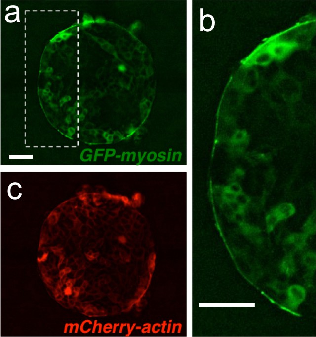
A supra-cellular acto-myosin cable sets the boundary of the colony.
(a) Madin Darby Canine Kidney (MDCK) cells expressing GFP-myosin and mCherry-actin. (b) Inset of the myosin cable at the colony boundary. (c) Image of the actin signal. Scale bar 50 µm.
Figure 4—figure supplement 2
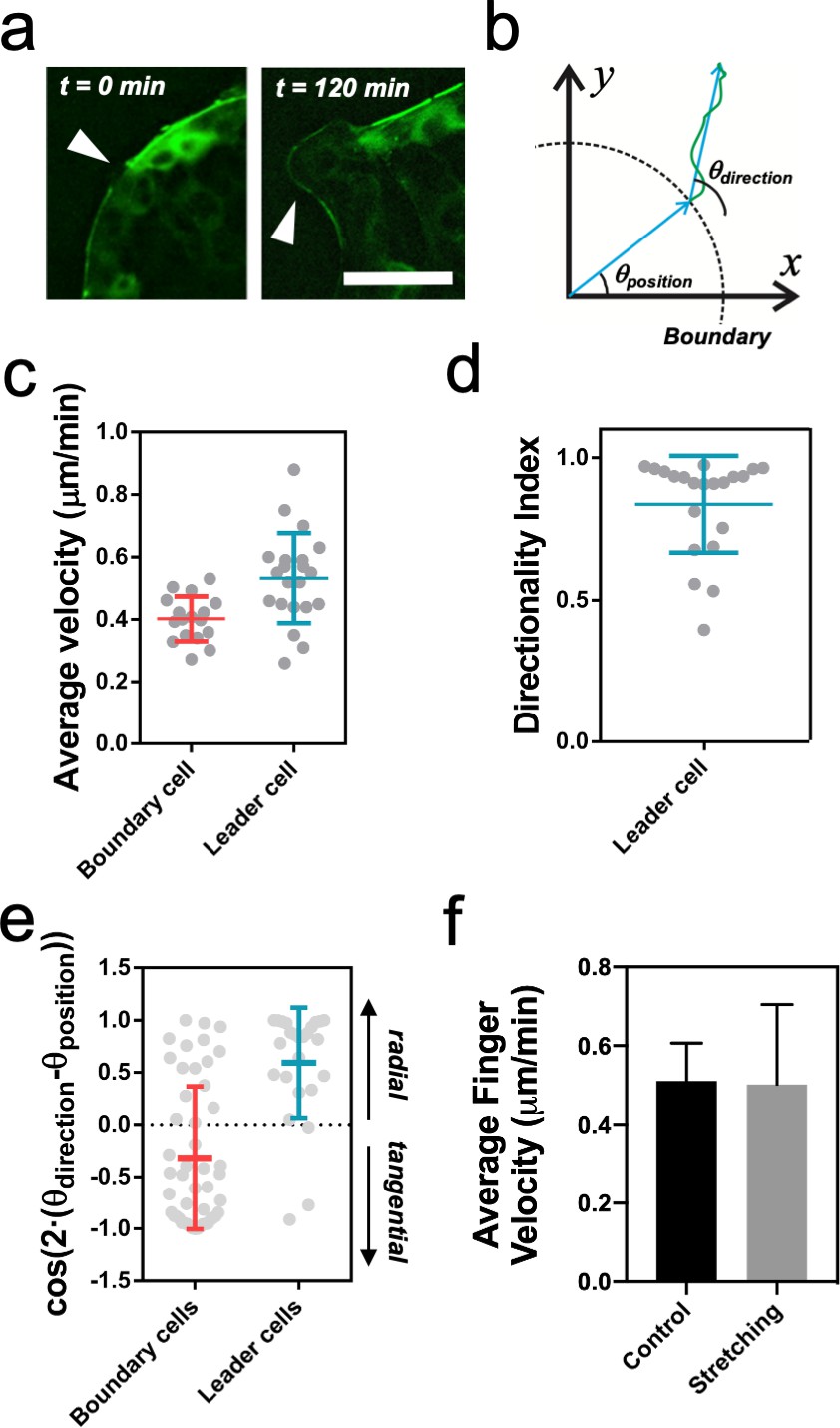
Leader cell dynamics.
(a) Discontinuities in the myosin cable structure at t = 0 min (white arrows) become finger-like structures at t = 120 min (white arrows). Scale bar 50 µm. (b) Schematics of a cell trajectory. Its initial position at the boundary with respect to the center of the colony defines the angle θposition. The vector between the initial and the final position of the cell defines the trajectory direction θdirection. (c) Average velocity of cells at the outer rim of the colony. Leader cells are faster than other boundary cells. nboundary = 17 cells from 8 colonies and N = 4 independent experiments and nleader = 21 cells from 12 colonies and N = 5 independent experiments. Individual cells in gray with Mean ± SD. (d) Directionality index for leader cells as the ratio of the distance between the initial and final position over the total distance covered by the cell. nleader = 21 cells from 12 colonies and N = 5 independent experiments. Individual cells in gray with Mean ± SD. (e) Cosine of two times the angle difference between θposition and θdirection for cells at the boundary and cells in finger-like structures. Values close to one correspond to radial trajectories and values close to −1 correspond to tangential trajectories. Mean value ± standard deviation, nboundary = 49 cells from 8 colonies and N = 4 independent experiments and nleader = 25 cells from 12 colonies and N = 5 independent experiments. Individual cells in gray with Mean ± SD. (f) Average finger velocity in control and in stretching cases. Only fingers parallel to the direction of stretching (Δθ < 30°) from Figure 4d are considered. Mean ± SD.
-
Figure 4—figure supplement 2—source data 1
Datasets for the individual velocities, angles and directionality index plotted in panels (c–f).
- https://cdn.elifesciences.org/articles/57730/elife-57730-fig4-figsupp2-data1-v2.xlsx
Figure 5 with 5 supplements
Collective effects and symmetry breaking.
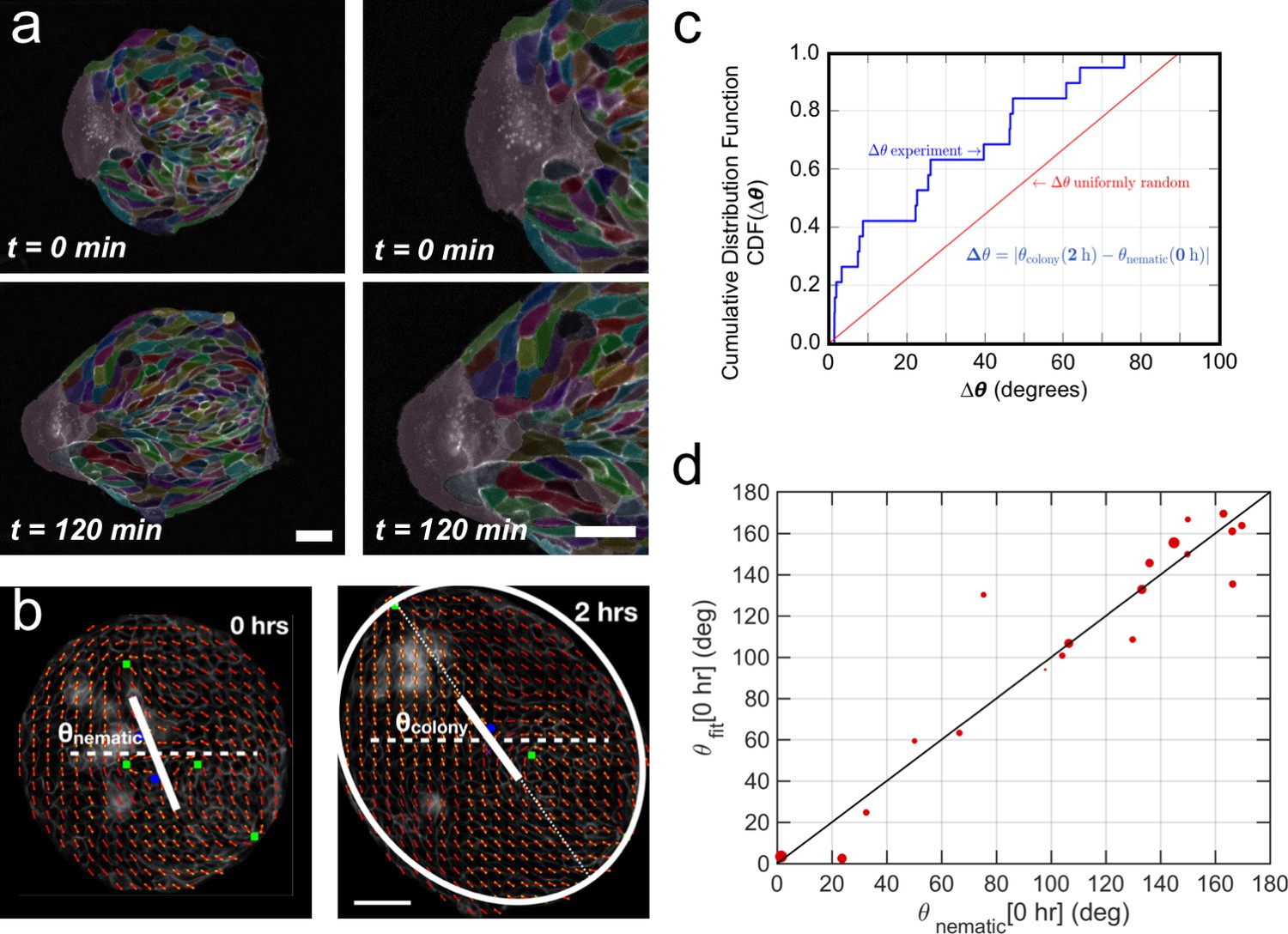
(a) A leader cell at the boundary of the colony pulls the colony outwards while inner cells deform and elongate. Scale bar 50 µm. (b) Cell shape is quantified using a nematic field (red segments). First, the mean cell shape nematic is quantified at the moment of stencil removal (0 hr) and the orientation θnematic of its mean for the entire colony is obtained. Then, the overall shape of the colony after 2 hr is obtained by fitting an ellipse, whose major axis makes an angle θcolony. The yellow directors correspond to fits for the cell shape nematic field obtained with respect to the +1/2 and −1/2 topological defects of the experimentally obtained (red) nematic field (also see Appendix 1D for details.) Scale bar 50 µm. (c) The cumulative distribution function (CDF) for the difference Δθ between θnematic (0 hr) and θcolony (2 hr) is obtained from n = 19 colonies of N = 5 independent experiments. Red line corresponds to the CDF of a random distribution of the difference Δθ. This plot shows a strong correlation between the cell shape nematic and the overall shape symmetry breaking (also see Figure 5—figure supplement 2d, and Appendix 1E). (d) The experimentally measured angle of mean nematic orientation θnematic obtained for 19 colonies at t = 0 hr is compared with its counterpart θfit obtained by fitting the experimental data with Equation 1 of the main paper with respect to the orientation parameter α (see Appendix 1D). The size of the red circles in (b) is proportional to the magnitude of anisotropy of the colony shape after 2 hr. n = 19 colonies of N = 5 independent experiments for MDCK.
-
Figure 5—source data 1
Raw data corresponding to panels (c) and (d).
For panel (c), we list the individual values used to calculate the cumulative distribution function. For panel (d), we list the values for the x-axis, the y-axis and the weight associated to each dot.
- https://cdn.elifesciences.org/articles/57730/elife-57730-fig5-data1-v2.xlsx
Figure 5—figure supplement 1
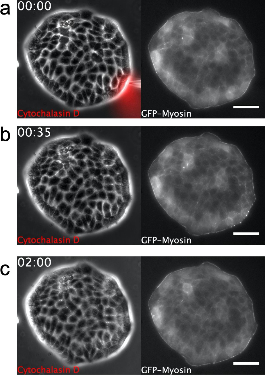
Supra-cellular acto-myosin cable disruption.
Phase contrast images of a Madin Darby Canine Kidney (MDCK) colony expressing GFP-myosin. A micropipette is placed shortly next to the colony boundary in (a). Note dynamics of myosin cable at the boundary. Scale bar 50 µm. Time: hh:mm. (a) Cytochalasin D is locally injected. (b) Disassembly of the myosin cable. (c) Recovery after Cytochalasin D injection. The myosin cable reforms at the colony boundary and no growth of finger is observed (see also the full dynamics in Video 5).
Figure 5—figure supplement 2
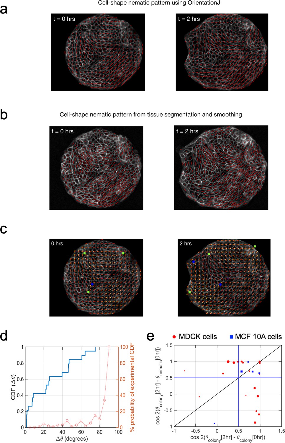
Cell shape nematic field.
Comparison of (a) cell shape nematic field obtained from OrientationJ plugin of ImageJ with (b) its counterpart obtained from tissue segmentation, triangulation and smoothing. It can be seen that the simpler, direct approach in (a) shows a very similar output as from the more detailed procedure in (b). (c) Fitting of cell-shape nematic field (yellow segments) with the one obtained experimentally (red segments) from OrientationJ using a simple expression (Equation 14 in Appendix 1D) in terms of topological defects. The green squares and the blue circles represent, respectively, +1/2 and −1/2 topological defects at the corresponding locations obtained from the experimental nematic field. (d) Correlation between θnematic (0 hr) and θcolony(2 hr) for finite sample size. Simple calculation to obtain the probability of observing a cumulative distribution function (CDF) for Δθ, the angle between the mean colony shape nematic θnematic at 0 hr and overall colony elongation θcolony at 2 hr, in the absence of any physical correlation between these two quantities, that is Δθ is picked with uniform probability from the set [0°, 90°] (orange curve and y axis on the right). It can be seen that in such a case, the probability to experimentally observe CDF >0.6 for Δθ = 30° in a sequence of 19 independent experiments is less than 1/100. This provides a strong indication that θnematic(0 hr) is very likely to be physically connected with θcolony(2 hr) and not randomly picked between 0° and 90°. n = 19 colonies of N = 5 independent experiments. (e) Final orientation of the colony is correlated with the initial shape nematic of initial orientation. The orientation of mean cell shape nematic θnematic of the colony at 0 hr is strongly correlated with the overall orientation of the colony θcolony at 2 hr. It can be inferred from the presence of 17 out of 26 colonies above the horizontal blue line at 0.5 (corresponding to Δθ = 30°). Of the rest of the nine colonies which do not show this trend, seven colonies show a strong correlation of their final orientation with their orientation at the start of experiment. The size of the symbols is proportional to the magnitude of anisotropy of the colony shape after 2 hr. nMDCK = 19 colonies of NMDCK = 5 independent experiments. nMCF 10A = 5 colonies of NMCF 10A = 2 independent experiments.
-
Figure 5—figure supplement 2—source data 1
Values of the probability to obtain the experimental cumulative distribution function of Figure 5c and we list the values for the x-axis, the y-axis and the weight associated to each point of Figure 5—figure supplement 2e.
- https://cdn.elifesciences.org/articles/57730/elife-57730-fig5-figsupp2-data1-v2.xlsx
Figure 5—figure supplement 3
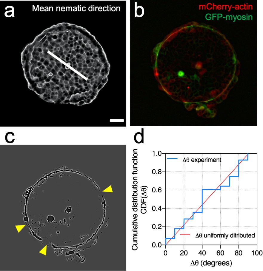
Mean nematic direction and defects in the acto-myosin cable.
(a) Mean cell shape nematic of a Madin Darby Canine Kidney (MDCK) colony. Scale bar 50 µm. (b) Actin (red) and myosin (green) signals at the boundary of the colony. (c) Processed image to identify openings of the cable (yellow arrows). (d) Cumulative distribution function of Δθ. Where Δθ corresponds to the angular distance between the mean nematic direction and the position of defects in the acto-myosin cable, . N = 3 experiments, n = 7 colonies.
-
Figure 5—figure supplement 3—source data 1
Values of the experimental data points used to obtained the cumulative distribution function showed in Figure 5d.
- https://cdn.elifesciences.org/articles/57730/elife-57730-fig5-figsupp3-data1-v2.xlsx
Figure 5—figure supplement 4
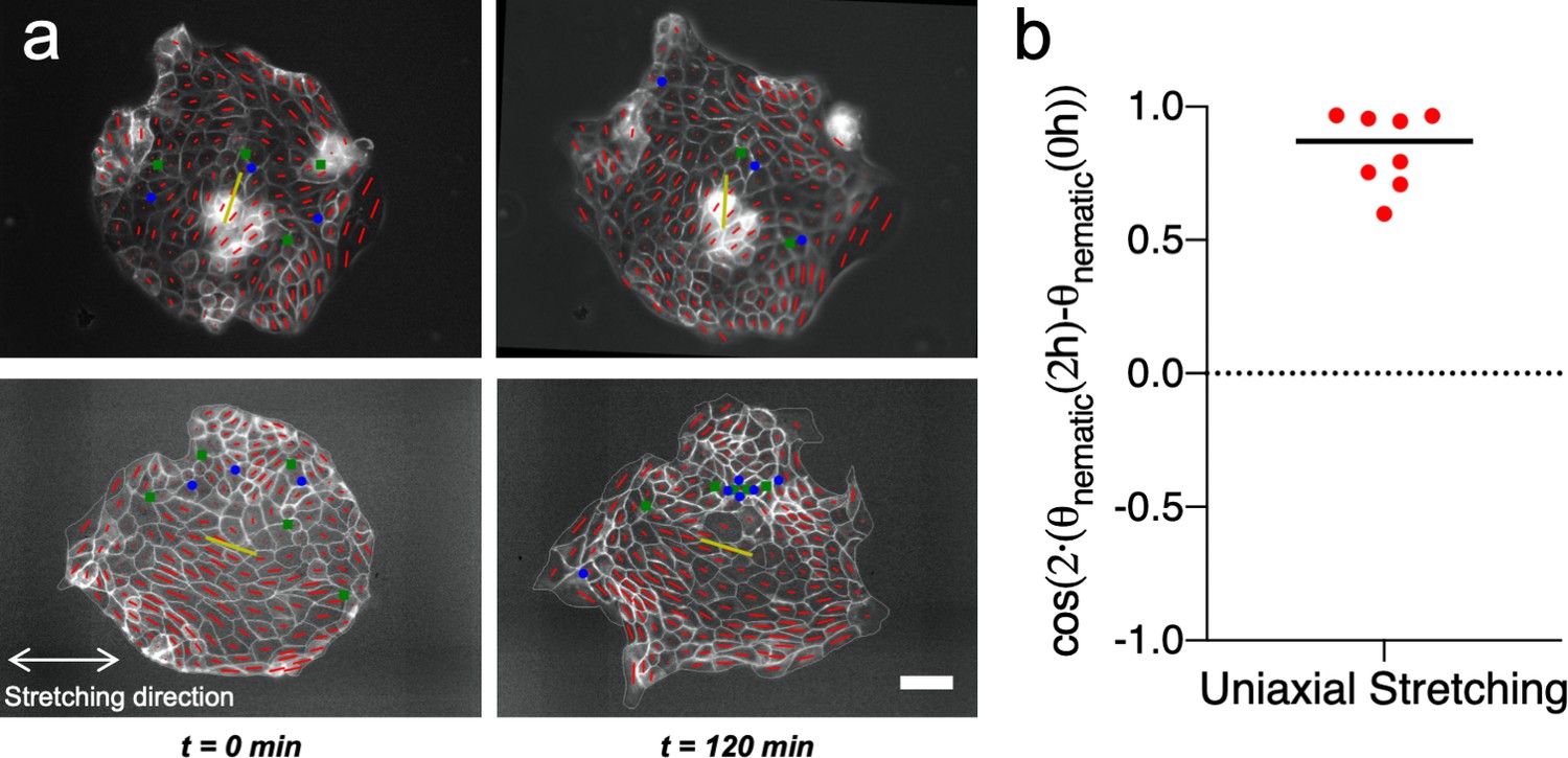
Uniaxial cyclic stretching does not modify the mean nematic direction.
(a) Cell shape nematic field (red segments) and mean nematic direction (yellow) of two colonies under uniaxial cyclic stretching at t = 0 min and t = 120 min. Mean nematic direction remains invariant after 2 hr of uniaxial cyclic stretching. Scale bar 50 µm. (b) Box plot of the change in the mean nematic direction of colonies under uniaxial cyclic stretching, cos(2·(θnematic (2 hr) – θnematic (0 hr))). n = 8 colonies from N = 6 experiments.
-
Figure 5—figure supplement 4—source data 1
Individual values represented in Figure 5b.
- https://cdn.elifesciences.org/articles/57730/elife-57730-fig5-figsupp4-data1-v2.xlsx
Figure 5—figure supplement 5
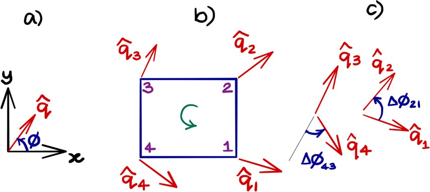
Obtaining topological charge for the orientation field on a rectangular grid.
(a) An orientation director makes an angle ϕ with the axis as shown. (b) The orientation field at the nodes of the smallest cell of the rectangular grid. The topological charge of within the cell is obtained by calculating the change in the orientation angle between the adjacent nodes of the grid and traversed in the anticlockwise direction. (c) The angle is taken to be the smallest of the angles between the adjacent directors and respects the nematic nature (or and symmetry) of the field. We note that this procedure is ambiguous when is a multiple of π/2, a case that generally does not happen in practice. After using anticlockwise and clockwise , the net topological charge of the orientation field within the rectangular cell in (b) is obtained as .
Figure 6 with 3 supplements
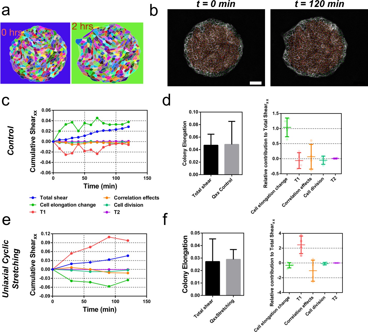
Contributions to symmetry breaking.
(a) Snapshots of two colonies from control condition segmented and tracked for cells using Tissue-Analyzer (TA) for a duration of t = 120 min starting from removal of stencil at t = 0. Scale bar 50 µm. (b) The segmented and tracked images are triangulated in Tissue-Miner (TM). Scale bar 50 µm. The green dots represent the centers of the segmented cells. (c) The dynamics of triangulation is analyzed in TM to provide the overall xx component of cumulative pure shear strain in a sample colony as a function of time (total shear). (d) Comparison between the mean total pure shear obtained from TM and the overall colony pure shear obtained from ellipse fitting (left). Total shear corresponds to ncolonies = 4 colonies from N = 2 independent experiments and Qxx control was obtained from ncolonies = 25 colonies of N = 11 independent experiments. Relative contribution of the different processes to the total pure shear (right). Total shear and contributions were obtained from ncolonies = 4 colonies from N = 2 independent experiments. (e) Cumulative pure shear decomposition for stretched colony. (f) Comparison between the mean total pure shear obtained from TM and the overall colony pure shear obtained from ellipse fitting (left) and relative contribution of the different processes to the total pure shear (stretching case). Total shear corresponds to ncolonies = 4 colonies from N = 4 independent experiments and Qxx stretching was obtained from ncolonies = 20 colonies of N = 9 independent experiments. Relative contribution of the different processes to the total pure shear (right). Total shear and contributions were obtained from ncolonies = 4 colonies from N = 4 independent experiments.
Figure 6—figure supplement 1
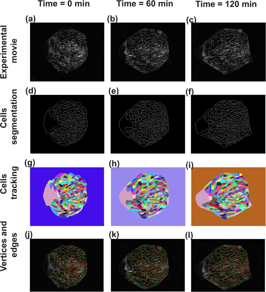
Steps in image analysis.
As the first step of analysis using TissueMiner, the images obtained from the experiment have been skeletonized, segmented and tracked using TissueAnalyser. (a–c) Show the images of cell colony at three different time points. (d–f) In order to differentiate the cell edges from the rest of the tissue for easy edge detection, the tissue has been skeletonized by adjusting the threshold value. (g–i) TissueAnalyser detects the edges and segments the colony, based on a watershed algorithm. At this step, algorithm also tracks the cells and assigns them a color and a global track identity, which remain constant throughout the process. When a cell undergoes division, a new track identity and color are assigned to one of the two daughter cells, while keeping the other same. (j–l) Using the output from TissueAnalyser, TissueMiner analyzes the tissue and represents it as a collection of cells made of a network of edges (green lines) connected to vertices (red dots) at any given time.
Figure 6—figure supplement 2
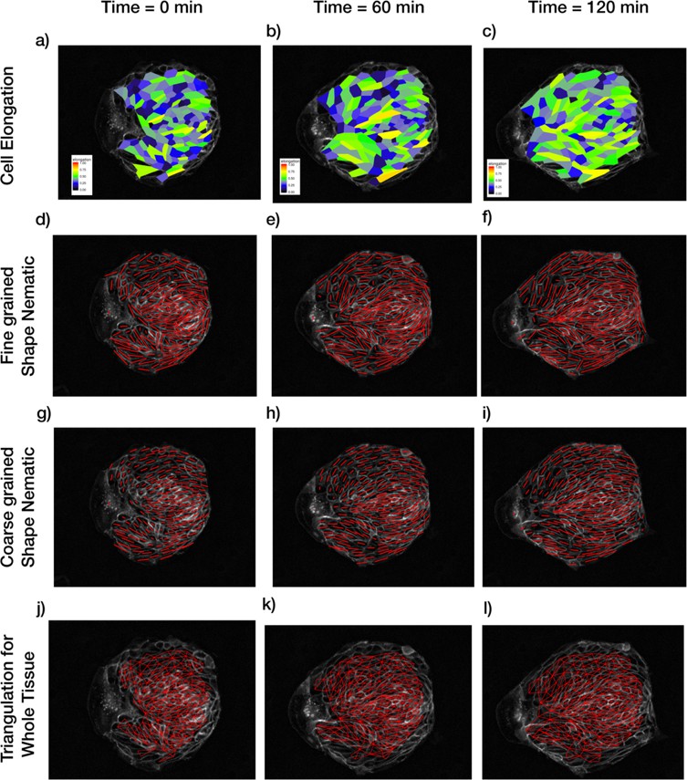
Patterns of cellular parameters obtained from TissueMiner analysis.
(a–c) Cell elongation magnitude distribution is plotted for three different time points. (d–f) Actual fine-grained cell elongation nematic for individual cells. The length of the segments is proportional to the magnitude of cell-shape nematic ε and the orientation is φ (see Appendix 1A). (g–i) Coarse-grained cell shape nematic is obtained by using a Gaussian kernel of size 30 pixels around every cell. (j–l) The algorithm to find out tissue deformation is based on the triangulation method as described in Etournay et al., 2016; Merkel et al., 2017. Any topological changes in the form of T1 transition, cell division, or cell extrusion will lead to a new triangulation. The triangulation is not reliable near the boundary and hence a layer of cells near the boundary is not included in the triangulation and subsequent calculations for tissue pure shear.
Figure 6—figure supplement 3
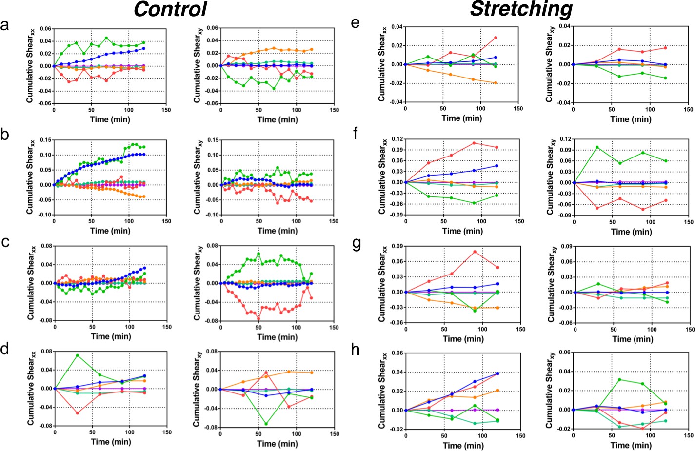
Cumulative pure shear decomposition.
(a–d) Control experiments. Decomposition of pure shear (blue) into its components arising from cell shape change (green), T1 transitions (red), correlation effects (orange), cell division (turquoise), and cell extrusion (purple). The x direction for each colony is chosen such that xy component of total shear is zero at t = 120 min, and indicates the overall orientation of colony anisotropy. The anti-correlation effect between cell elongation and other components that is seen in Figure 6c of the main paper is clearly visible in every case. The interval between subsequent time data points is 10 min for (a), 5 min in (b–c), and 30 min for (d). The data for xx component of pure shear in (a) is presented in Figure 6. (e–h) Stretched colonies. Same analysis method and time evolution of pure shear presented in (a–d) for control colonies, but now for stretched colonies. The time interval between subsequent time data points is 30 min. Interestingly, the anti-correlation effect between the cell elongation and other components with respect to the total pure shear is seen here too.
-
Figure 6—figure supplement 3—source data 1
Values of each of the different contributions to cumulative shear along time for the 8 colonies shown in Figure 6—figure supplement 3.
- https://cdn.elifesciences.org/articles/57730/elife-57730-fig6-figsupp3-data1-v2.xlsx
Figure 7 with 1 supplement
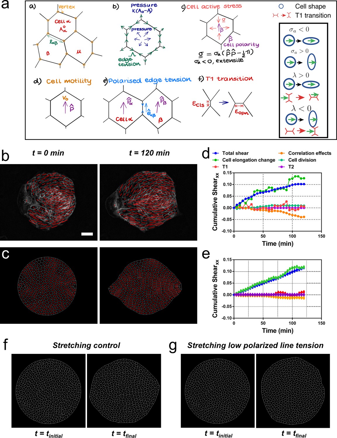
Vertex model recapitulates symmetry breaking and shear decomposition.
(a) Schematic of vertex model depicting the arrangement of cells, forcing, and topological transitions in a tissue. 2-D monolayer of epithelial cells is represented by polygons, generally sharing a common edge and two vertices between cells. For any cell α shown in the figure, Aα is the area, is the preferred area and lαβ is the length of the edge shared between cells α and β. The forces on any vertex i in the basic vertex model are from pressure due to deviation in the cell area from its preferred value and the tensile force arising from edge or cortical contractility Λ. In our model, each cell also has a polarity associated with it through which active forces can act on the cell vertices due to anisotropic cell active stress (extensile in our case), cell motility v0 and polarized or biased edge tension that depends on the orientation of the edge with respect to the polarities of the adjoining cells. When the edge connecting two cells becomes smaller than a critical value , the cells are made to modify their neighbors by forming a new edge of length as shown. Scheme depicting the different possibilities from the model parameters. (b) Experimental coarse-grained cell shape nematic at t=0 and t=120 min. Scale bar 50 µm. (c) A vertex model with internal activity arising from extensile active cell stress (σa′ = -5) and biased edge tension for the cell-cell junctions (λ′ = 20). Prime symbol ′ refers to non-dimensional values (see Appendix 2E). (d) Overall xx component of cumulative pure shear strain in the sample colony shown in (b) as a function of time (total shear). (e) Shear decomposition of the in silico experiment which is similar to its experimental counterpart in (d). (f) A vertex model with an additional aligning term that defines the direction of the uniaxial stretching through cell polarity. When cell-cell junctions are intact, biased edge tension (λ′ = 50) dominates over active cell stress (σa′ = 2) and the colony elongates along the (horizontal) direction of stretch collectively through T1 transitions. (g) When the effect of edge tensions is lowered (λ′ = 25) and active cell stress is increased (σa′ = 4), the colony elongates perpendicularly to the direction of stretch.
Figure 7—figure supplement 1
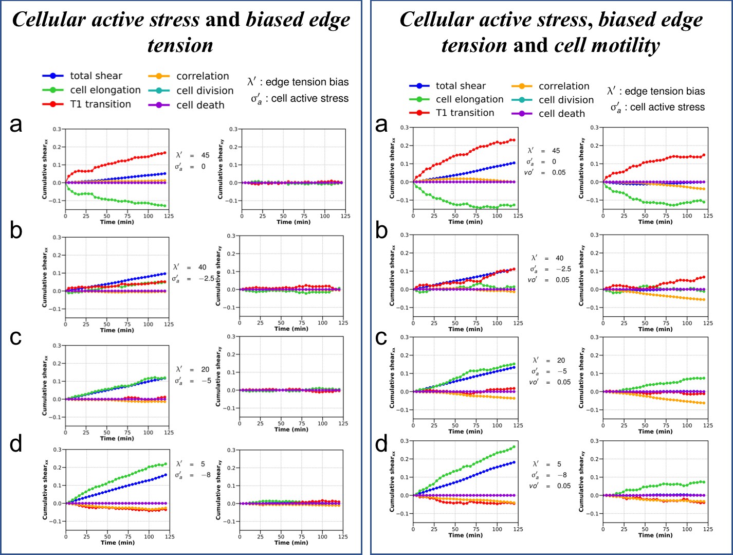
Cumulative pure shear decomposition patterns for the simulated colonies.
(Left) Varying strength of cellular active stress and biased edge tension. Briefly, the cellular active stress () is an internal cellular stress that tends to drive cell elongation. Biased edge tension () is implemented by modulating the line tension of the cell edges on the basis of the relative angle the edges make with the polarity of their two shared cells. A colored noise with a small strength and persistence time is applied on the edge line tension to ensure baseline fluctuations. Note the relative positions of the pure shear due to T1 transitions (red) and cell elongations (green) with respect to the overall colony shear (blue). The x axis is chosen to be the major axis of elongation such that the xy component of cumulative total pure shear strain is zero at the end of the simulation. It can be seen from (a) to (d) that the relative position of the red and green curves with respect to the blue curve is an indication of the internal processes which are more dominant in a particular colony and show marked similarity with the corresponding experimental curves seen in Figure 6—figure supplement 3. (Right) Varying strength of cellular active stress, biased edge tension and cell motility. All simulations shown here are as in left panel a–d, but with the addition of a small motility term . It can be clearly seen that addition of motility does not qualitatively modify the relative positions of the contributions from cell elongation (green) and T1 transitions (red) with respect to each other when compared with their counterparts in left panel. However, in this particular case, for the parameters and the initial conditions, the xy component of the shear is comparatively more dominant.
-
Figure 7—figure supplement 1—source data 1
Values of each of the different contributions to cumulative shear along time for the different simulations.
- https://cdn.elifesciences.org/articles/57730/elife-57730-fig7-figsupp1-data1-v2.xlsx
Figure 8 with 1 supplement
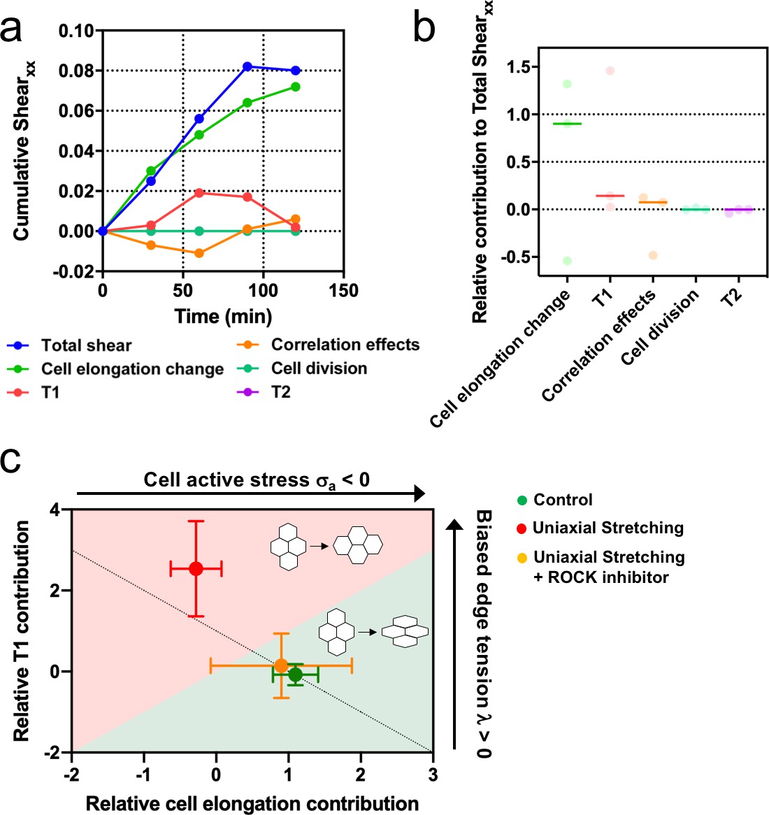
Stretching-dependent elongation is mediated by ROCK.
(a) Cumulative pure shear decomposition for stretched colony in the presence of ROCK inhibitor Y-27632 50 µM. (b) Relative contribution of the different processes to the total pure shear. Total shear and contributions were obtained from ncolonies = 3 colonies from N = 3 independent experiments. Individual experiments and median are plotted. (c) Contribution of single-cell elongation to total elongation versus contribution of T1 transitions to total elongation. In the green area, single-cell elongation dominates over T1, whereas red area corresponds to T1 transitions dominating over cell elongation. Along the dashed line, contribution of correlation effects and oriented cell division to total shear is close to zero. Above this line this contribution is negative and below the line is positive. According to our vertex model, by changing the strength of cellular active stress and biased edge tension, colonies change the relative contribution of each mechanism of elongation. Experiments show that epithelial colonies spontaneously elongate through single-cell elongation (green point, N = 2, ncolonies = 4), whereas colonies under uniaxial stretching elongate through T1 (red dot, N = 4, ncolonies = 4). When ROCK activity is inhibited, colonies under uniaxial stretching elongate through single-cell elongation (orange dot, N = 3, ncolonies = 3). Points represent median ± SD.
-
Figure 8—source data 1
Values of each of the different contributions to cumulative shear as time progresses for the three colonies analyzed.
- https://cdn.elifesciences.org/articles/57730/elife-57730-fig8-data1-v2.xlsx
Figure 8—figure supplement 1
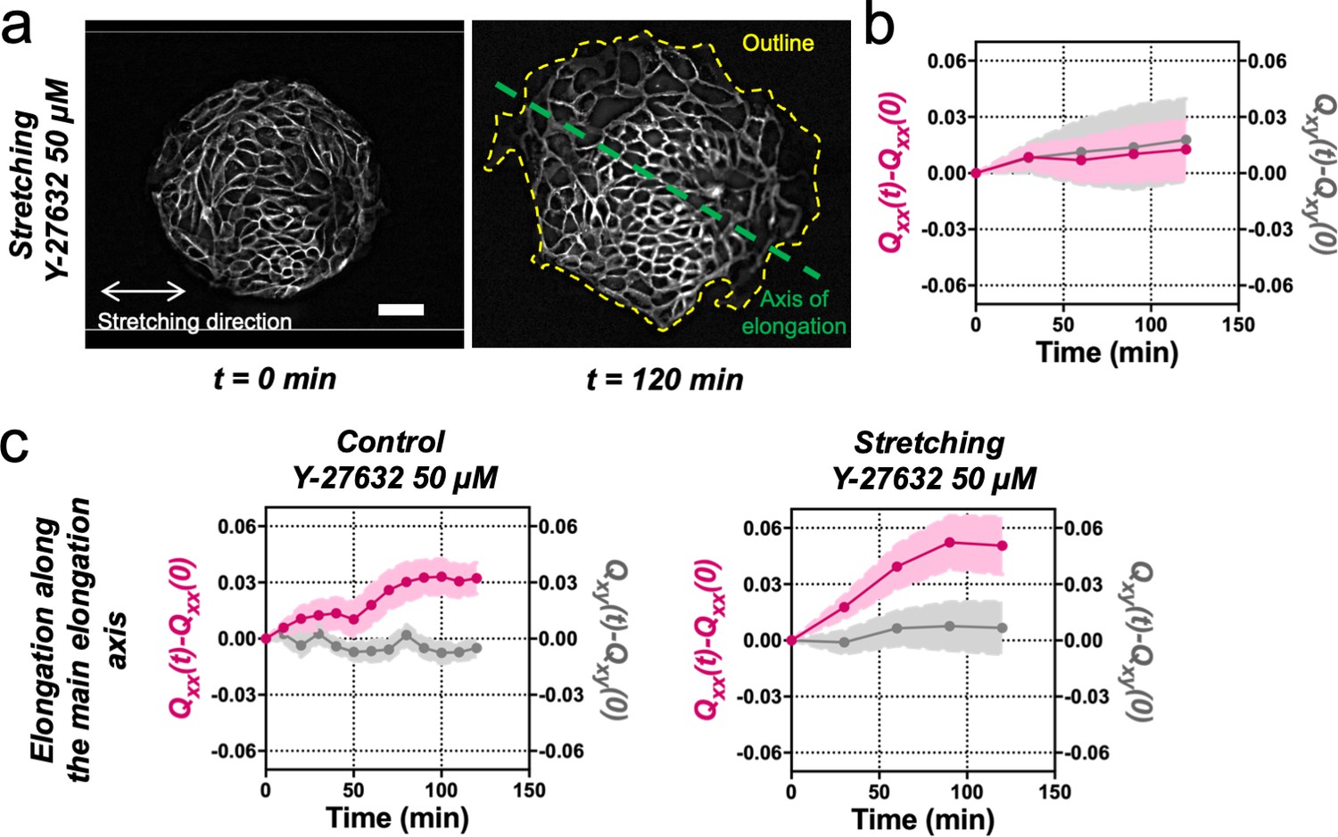
Stretching-dependent elongation is mediated by ROCK.
(a) Fluorescent images of an Ecadherin-GFP Madin Darby Canine Kidney (MDCK) colony evolving for 120 min under cyclic mechanical stretching when ROCK is inhibited by Y-27632 50 µM. The direction of the uniaxial stretching is indicated in white, the outline of the colony at 120 min is indicated in yellow and the major axis (θ(tfinal)) is indicated in green. Colonies do not elongate along the stretching direction, but they still have a main elongation axis. Scale bar 50 µm. (b) Qxx (left y axis) and Qxy (right y axis) of MDCK colonies during 120 min of cyclic uniaxial stretching in the presence of ROCK inhibitor. Elongation is measured in the direction of external force (α = 0). Mean value ± standard error of the mean. N = 3, n = 8 colonies. (c) Comparison of the cumulative Qxx (left y axis) and cumulative Qxy (right y axis) during 120 min of colony expansion when ROCK is inhibited in control and under cyclic uniaxial stretching. Elongation is measured along the spontaneous elongation direction (α = θ(tfinal)). Mean value ± standard error of the mean, Ncontrol = 3, n = 12 colonies and Nstretching = 3, n = 8 colonies.
-
Figure 8—figure supplement 1—source data 1
Values of Qxx(t)-Qxx(0) and Qxy(t)-Qxy(0) for each of the colonies included in Figure 8—figure supplement 1.
- https://cdn.elifesciences.org/articles/57730/elife-57730-fig8-figsupp1-data1-v2.xlsx
Author response image 1
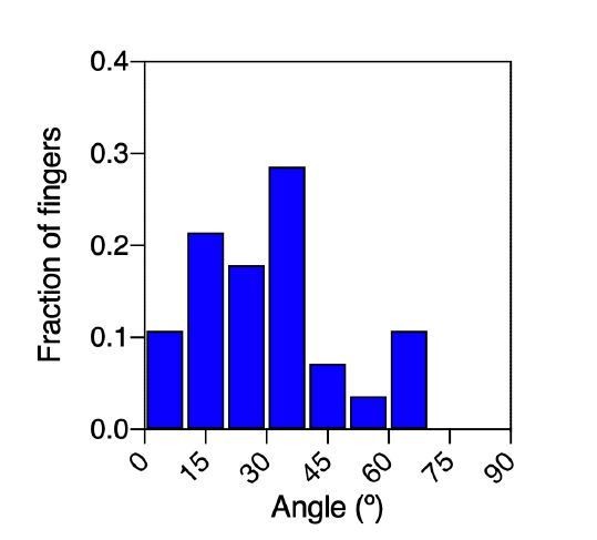
Distribution of the angular distance between fingers and their nearest defect.
Videos
Video 1
Spontaneous symmetry breaking of circular colonies.
Time-lapse of a Madin Darby Canine Kidney (MDCK) cells colony freely evolving after removal of a poly(dimethylsiloxane) (PDMS) stencil. Time in hh:mm. Scale bar 50 μm.
Video 2
Cyclic stretching of Madin Darby Canine Kidney (MDCK) colonies.
Time-lapse of an MDCK colony under cyclic stretching (5% and 120 s). Time in hh:mm:ss. Scale bar 50 μm.
Video 3
Expansion of Madin Darby Canine Kidney (MDCK) colonies under cyclic stretching.
Time-lapse of an MDCK colony under cyclic stretching (5% and 60 s) at the 0% strain position. Time in hh:mm. Scale bar 50 μm.
Video 4
Early symmetry breaking of circular colonies.
Composite array time-lapse of MDCK-GFP-Ecadherin cells colonies during the first 2 hr of expansion. Time in hh:mm. Scale bar 150 μm.
Video 5
Disruption of the acto-myosin cable.
Movie showing the disruption of the acto-myosin cable. The colony and the micropipette used are shown at the left and the myosin signal is shown at the right. Cytochalasin D was mixed with Cy5 to allow its visualization. Time in hh:mm. Scale bar 50 μm (right).
Video 6
Nematic field alignment precedes colony elongation.
Movie showing cell- shape nematics and topological defects of an elongating colony. Time in hh:mm. Scale bar 50 μm.
Video 7
Contributions to colony elongation.
Movie showing cell tracking, neighbor triangulation, cell-shape nematics, and topological defects of an elongating colony. Time in hh:mm. Scale bar 50 μm.
Video 8
In silico recreation of a colony elongation.
Vertex model simulation of a colony elongation. Cell-shape nematics, topological defects, and cell polarization are followed over time.
Video 9
In silico recreation of single versus collective effect of stretching.
Competition between active cell stress σa and biased junction tension λ governs direction of colony elongation. (Left) When cell-cell junctions are normal, we propose that λ’=50 dominates over σa′ = −2 and the colony elongates along the direction of stretch (horizontal) collectively through T1 transitions (collective stretching). (Right) When E-cadherin levels are low (blocked by anti-E-cadherin antibody), the effect of edge tensions λ′=25 is lowered as compared and that of active cell stress σa′ = −4 is increased, thus leading to elongation of the colony perpendicular to the direction of stretch (vertical) through individual cell elongation (single stretching). The superscript ′ indicates non-dimensionalized parameter (see Appendix 2E).
Additional files
Download links
A two-part list of links to download the article, or parts of the article, in various formats.
Downloads (link to download the article as PDF)
Open citations (links to open the citations from this article in various online reference manager services)
Cite this article (links to download the citations from this article in formats compatible with various reference manager tools)
Epithelial colonies in vitro elongate through collective effects
eLife 10:e57730.
https://doi.org/10.7554/eLife.57730


