Synaptic and intrinsic mechanisms underlying development of cortical direction selectivity
- Department of Biology, Brandeis University, United States
- Volen Center for Complex Systems, Brandeis University, United States
- Sloan-Swartz Center for Theoretical Neurobiology Brandeis University, United States
Figures
Figure 1
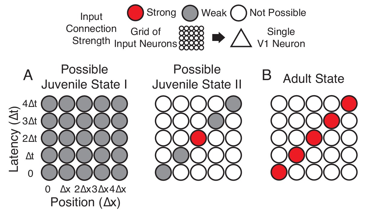
Hypotheses of initial naive states.
(A) In Possible Juvenile State I, receptive fields might be initially broad and weak in space and time and later sharpened to exhibit a slant. In this state, the lack of direction selectivity comes from the symmetry in the broad initial receptive field. In Possible Juvenile State II, there is a compact initial input that is constrained to grow only at certain positions and latencies, either by addition of new synaptic inputs or by changes in the properties of existing inputs. In this state, the lack of direction selectivity comes from the symmetry of compact strong input, and the weak inputs do not contribute at the naive stage. (B) Experienced state, with a characteristic directional slant in space time, indicating that the cell would respond to a leftward moving stimulus at an appropriate velocity.
Figure 2 with 1 supplement
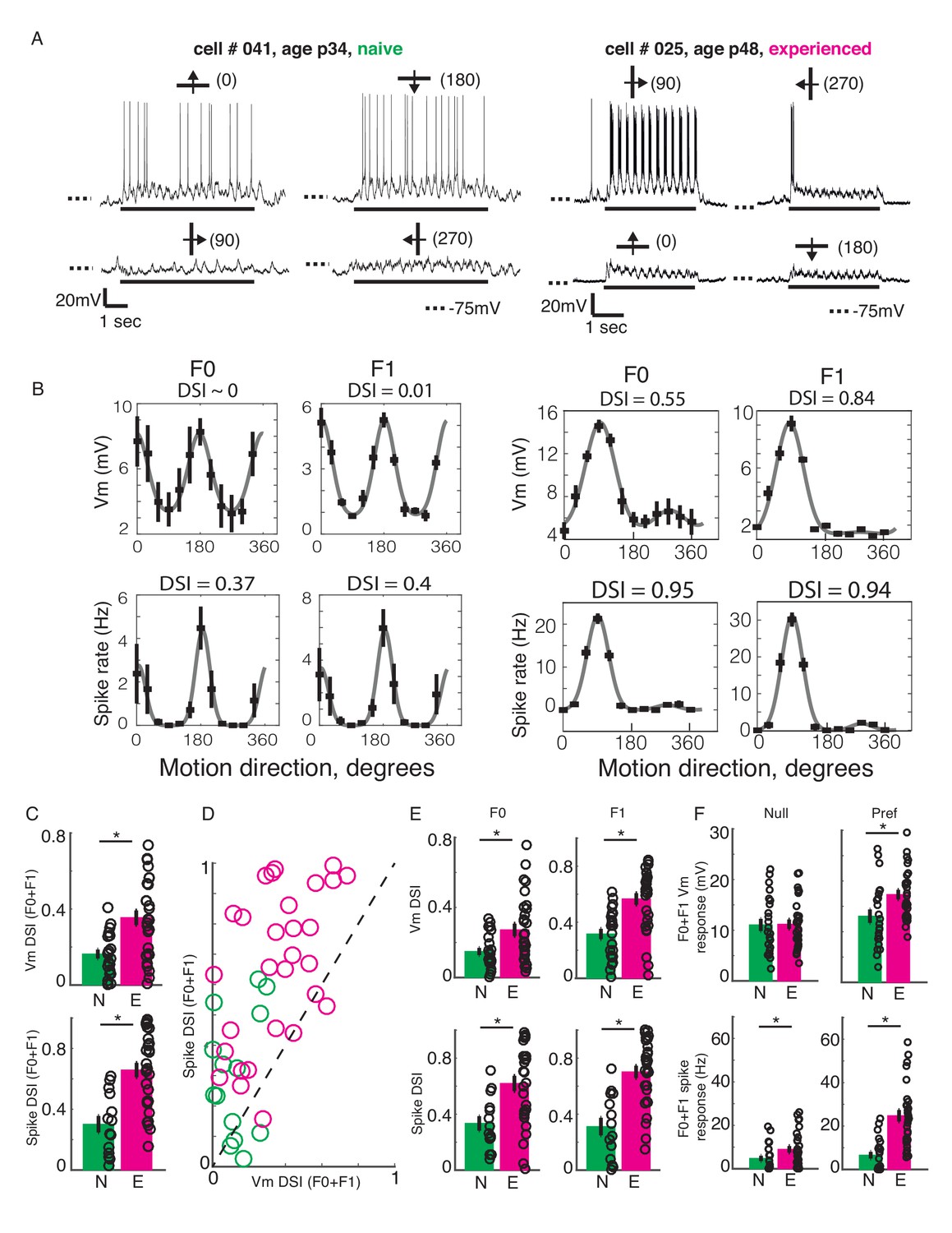
Developmental increase in direction selectivity of membrane potential (Vm) and spiking responses in V1 cells.
(A) Vm responses of a simple cell from a visually naive and an experienced ferret each. For each cell, single-trial responses to presentation of sinusoidal gratings moving in both directions orthogonal to the preferred orientation (top) and the non-preferred orientation (bottom) are shown. The stimulus orientations and motion directions are indicated above each trace with a solid bar and arrow, respectively, and the angles representing the specific directions of motion are given in parentheses. Solid bar below each trace indicates the duration of the stimulus display and dotted lines indicate the Vm level of −75 mV. For both cells, the gratings drifted at a temporal frequency of 4 Hz and the Vm oscillated at the same frequency with a strong response to each grating cycle. (B) Direction tuning curves of the cells in A, plotted separately for Vm (top) and spiking (bottom) responses, and for the F0 or DC (left) and the F1 or fundamental (right) components of the responses. Direction selectivity index (DSI) value calculated from each tuning curve is given above each curve. Both F0 and F1 DSI values are higher in the cell from the experienced animal. (C) Mean total Vm and spike DSI values, calculated from F0+F1 responses, compared between naive (N, green) and experienced (E, magenta) animal groups. (D) Vm and spike total DSI (F0+F1) values for each cell plotted against each other. Dashed line denotes the line of unity. (E) Same as C, but the DSI values are calculated separately for the F0 and the F1 components of response. (F) Mean total (F0+F1) Vm and spiking responses to the null and preferred direction of motion compared between naive and experienced groups. For all panels: error bars denote SEM; circles denote values for individual cells; asterisks denote significant differences at p<0.05 level, Wilcoxon rank sum test.
Figure 2—figure supplement 1
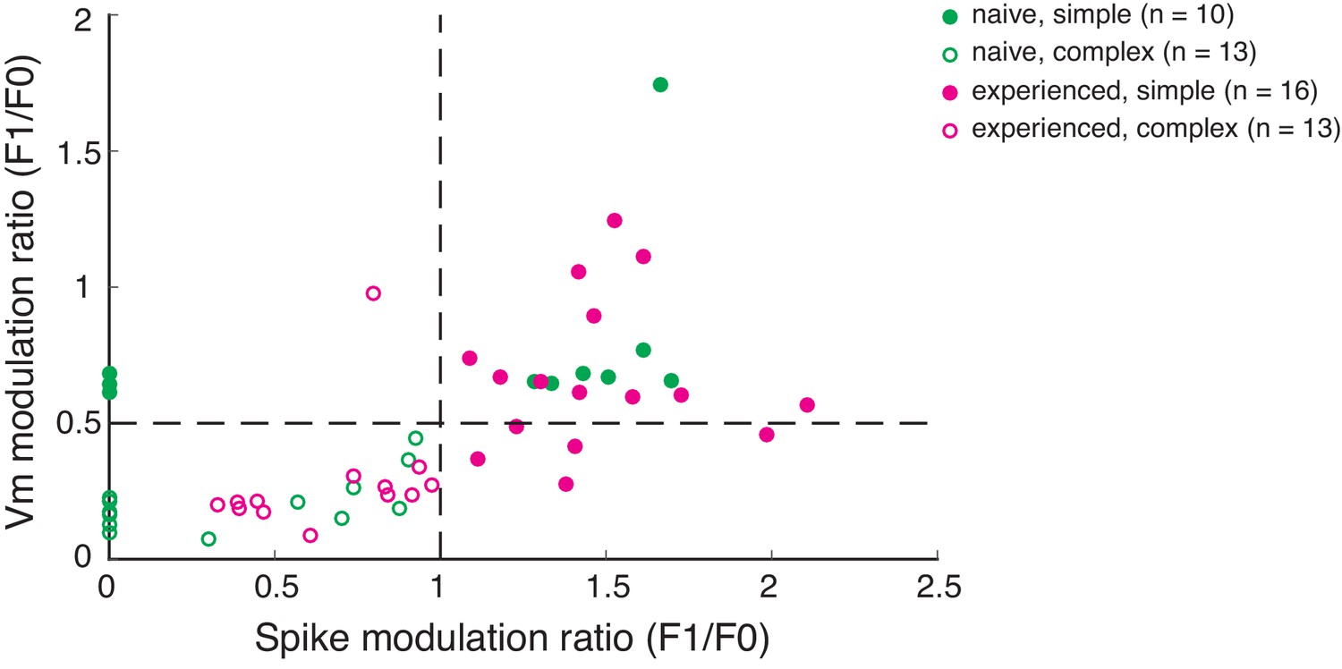
Scatterplot of spike and Vm modulation ratios (F1/F0) for allcells recorded.
Cells with spike modulation ratio >1 from this figure were classified as simple cells. In the naive group, many neurons did not fire sufficient spikes to calculate a spike modulation ratio. Those neurons were plotted in this figure with a spike modulation ratio set to 0. Out of those neurons, those with Vm modulation ratio >0.5 were classified as simple cells.
Figure 3
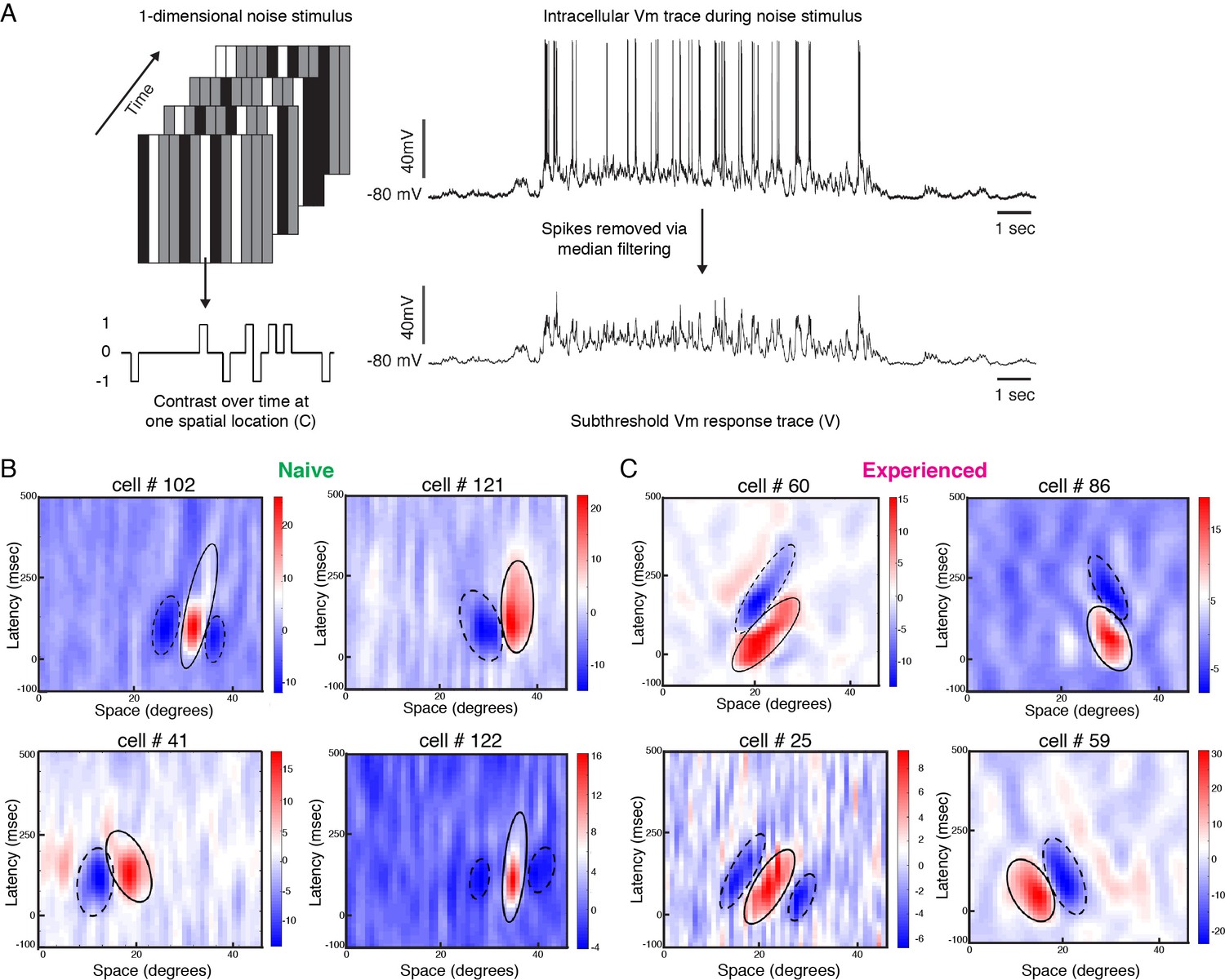
Developmental reorganization of linear spatiotemporal receptive fields in visual cortical simple cells.
(A) Schematic of sparse noise stimulus, rotated to match each cell’s preferred orientation. Spikes were removed and the membrane potential was correlated with the stimulus at each position. (B) Vm spatiotemporal receptive fields of four simple cells each from naive animals. X-axis represents spatial location, y-axis represents latency from onset of visual stimuli, and the cross-correlation coefficient between the stimulus contrast and Vm values are represented by the color. Black lines outline the ellipses fitted to the ON (continuous) and OFF (dashed) subunits. Raw correlations are shown, which are blurred by the time step of the stimulus (100 ms), so some ellipses overlap zero. (C) Same, for four cells from experienced animals. Receptive fields in experienced animals appeared more elongated in space time, and more slanted, consistent with the increased direction selectivity that was observed.
Figure 4 with 1 supplement

Spatiotemporal receptive fields become more extended, slanted in space-time with short-term visual experience.
(A) Quantification of the nine parameters defining the characteristics of the spatiotemporal receptive field subunits. In each panel, the parameter being quantified is described by a schematic on the left, and on the right is a bar plot showing the mean ± SEM of the parameter values in the naive (N, green, 19 subunits from 8 cells) and experienced (E, purple, 26 subunits from 12 cells) animals. Black circles denote individual subunit values. Red stars denote statistical significance at p<0.05 level via WRS test. (B) Relationship between cell-average spatiotemporal receptive field structure parameters and Vm DSI for all simple cells. The R2 and p values for each linear correlation are shown above each plot. Raw correlations were used in the calculations, which are blurred by the time step of the stimulus (100 ms), so some ellipses begin earlier than latency 0. If the outlier (orientation <45 °) in orientation is removed, then the r2 is 0.26 and p≤0.03. (C) All subunits (ON = solid, OFF = dashed) for naive cells. Lines are at 0 time lag. Scale bar shows 250 msec by 20° of visual angle. Note that correlations are raw, so they are blurred 100 ms by the stimulus timesteps (some subunits begin before time 0). (D) Same, for experienced cells. Note the earlier onset responses and the greater slants. (E) Cumulative histogram of response latencies of naive and experienced simple cells to grating stimuli. Latency is defined as the first time when the voltage signal reaches six standard deviations.
Figure 4—figure supplement 1
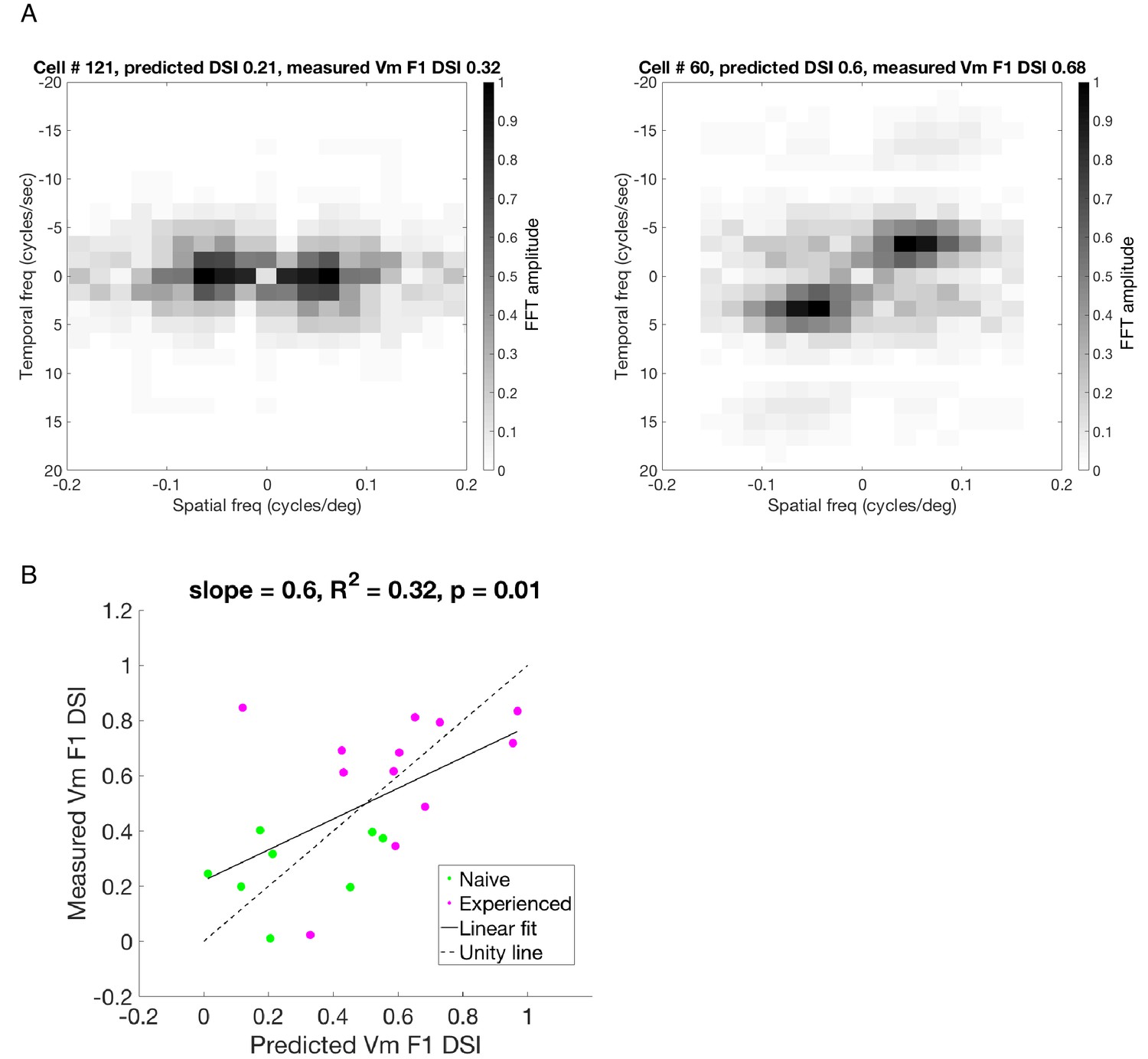
Predicting Vm DSI of the F1 component from the simple cell STRFs.
(A) STRFs were Fourier transformed along both space and time axes to convert both dimensions to the frequency domain. The amplitudes were scaled between 0–1 and plotted as a color map image, in which the intensity of every pixel represented the Fourier amplitude of response at a particular spatial and temporal frequency combination. The darkest pixel corresponds to the neurons’ preferred spatial and temporal frequencies. Left: frequency-domain STRF of cell # 121 recorded in a visually naive ferret; Right: frequency-domain STRF of cell # 60 recorded in a visually experienced ferret. In these images, there are four quadrants organized around the origin, which represents 0 spatial and temporal frequency. The two diagonally opposite quadrants contain the same data, and each of the two such diagonal pairs correspond to the two opposite directions of motion each. For example, if the quadrant with positive spatial and temporal frequencies represents forward motion, then the quadrant with positive spatial and negative temporal frequencies represents the backward motion. In a cell with low direction selectivity (left), the intensity of pixels in these two quadrants are similar, whereas in a highly direction selective cell (right), the pixel intensities are strikingly higher in one of the two quadrants. The imbalance of intensities along the two diagonals can be used to predict direction selectivity of the linear component for a simple cell. The summed amplitudes from each of the two quadrants represent predicted amplitudes of Vm responses to the two opposite motions, and we used those predicted responses to calculate a predicted Vm DSI for the linear component of the cell’s response. (B) The predicted Vm DSI of the linear component (F1) and the actual Vm F1 DSI measured in each cell were correlated to each other, and this was true for both the naive and the experienced groups. The overall R2 value of 0.32 implies that the linear spatiotemporal summation properties of the simple cells can account for 32% of the variance in Vm F1 DSI.
Figure 5
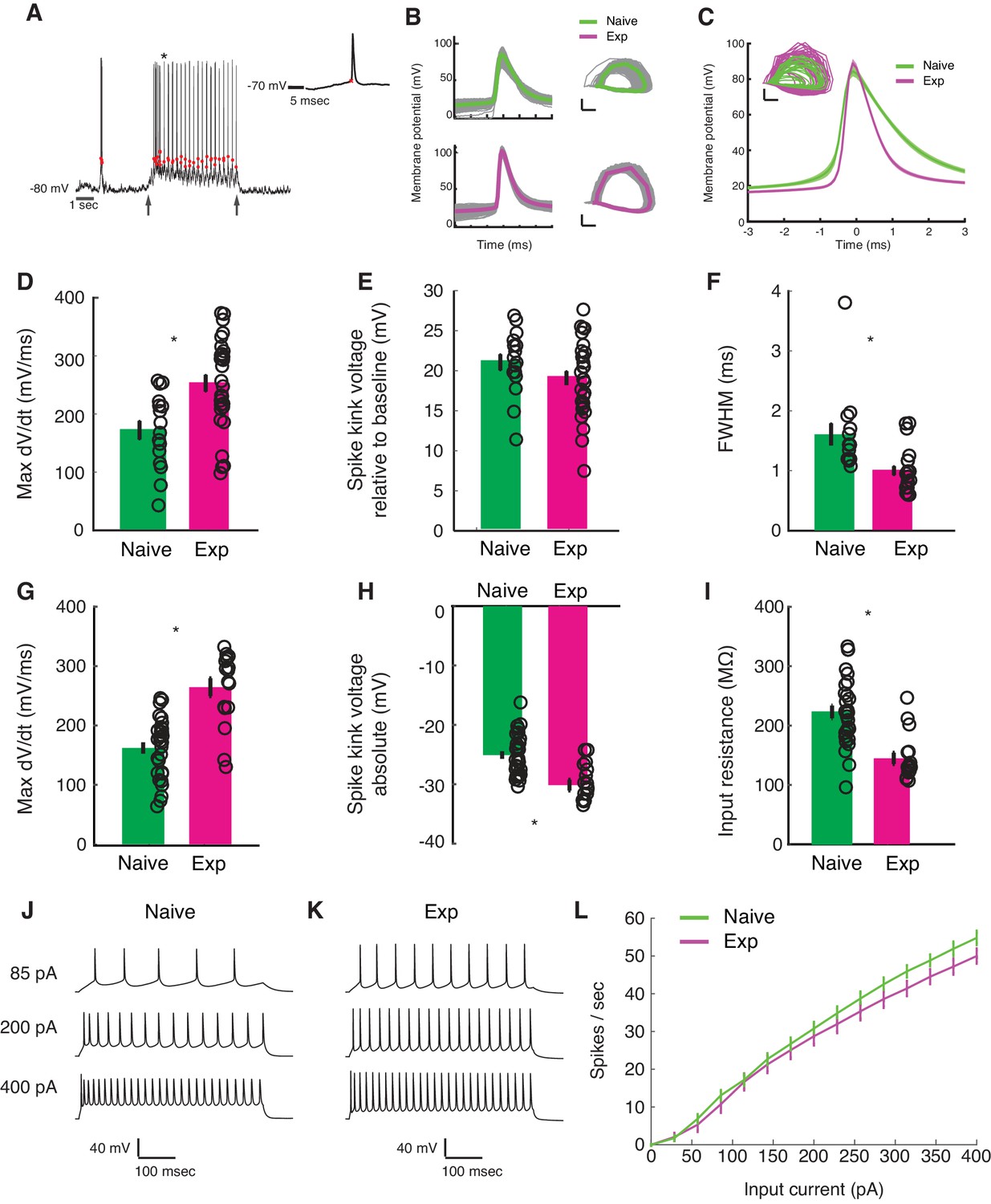
Developmental enhancement of excitability in cortical cells.
(A) Detection of spike kink voltage from single action potentials in vivo (Azouz and Gray, 1999). (B) Action potentials and spike phase diagram from an example naive (top) and experienced cell (bottom). Individual spike traces shown in gray. In spike phase diagram, membrane potential is on the horizontal axis (scale bar is 20 mV) and dV/dt is on the vertical axis (scale bar is 100 mV/msec). (C) Average and standard error of the mean of voltage waveforms for naive (N = 14) and experienced (N = 29) cells, showing much wider action potentials in naive animals. Shaded area is standard error of the mean across cells. Inset: phase diagram of mean spike waveforms; membrane potential is on the horizontal axis (scale bar is 20 mV) and dV/dt is on the vertical axis (scale bar is 100 mV/msec). (D) Maximum dV/dt for naive and experienced cells in vivo (WRS test, p<2.0e-04); (E) spike kink voltages in vivo (WRS test, p=0.2); (F) action potential full width at half height (WRS test, p<4.3e-04) in vivo. (G) Maximum dV/dt for synaptically isolated cells in brain slices for naive and experienced animals. Ex vivo measurements showed similar maximum dV/dt values as in vivo measurements (N = 29 naive, N = 17 experienced, WRS, p<2.4e-05), showing similar values as in vivo measurements. (H) Spike kink voltage exhibited a significant decrease when measured in isolated cells from visually experienced animals (WRS p<1.6e-04). (I) Spike kink reductions and increased maximum dV/dt co-occurred with developmentally typical decreases in membrane resistance (WRS, p<1.2e-04), suggesting that experienced cells would take longer to charge from rest even though they spike at lower voltages. Example firing rate vs. current curves for a cell from a naive (J) animal and an experienced (K) animal are shown, and average firing rate vs. current curves are shown (L). The increased excitability with age and the decreased input resistance produced firing rate vs. current relationships that were not different between the two cases: (Kruskal-Wallis test of slopes: p<0.068). For all panels, p-values as listed are before Bonferroni correction; significant * indicates significant difference after Bonferroni correction (which did not change results for these tests).
Figure 6 with 1 supplement
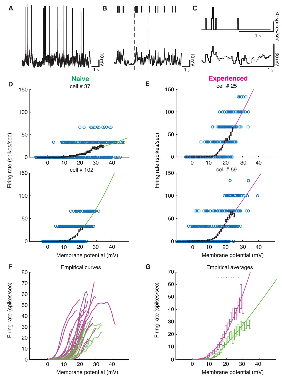
Developmental enhancement of input-output gain.
(A) To calculate the voltage-to-firing rate transform, we (B) extracted spike times and used median filtering to remove spike waveforms from the membrane potential, and (C) averaged firing rate and spike-filtered membrane potential into 30 ms bins (Priebe et al., 2004; Priebe and Ferster, 2005; Priebe and Ferster, 2006). (D) Membrane potential and firing rate observations from two cells from naive and (E) two cells from experienced animals. Empirical means and standard error of the mean in sliding 1 mV windows (black) and a power law fit (Priebe et al., 2004) (naive are green, experienced are magenta) are shown for each cell. Empirical means are calculated up until first bin that does not contain 15 Vm, firing rate ordered pairs. (F) Empirical mean voltage-to-firing rate relationships for all cells (N = 16 naive, N = 29 experienced). (G) Mean and standard error of the mean empirical voltage-to-firing rate transforms for naive and experienced animals, averaging over cells; * indicates locations where a t-test shows a p-value of less than 0.05. Voltage values that had data for at least two cells are shown. Experienced voltage-to-firing rate transforms exhibited increased firing rates at a given voltage over a large membrane voltage range. Solid lines are power law fits, weighed by number of data points at each voltage.
Figure 6—figure supplement 1
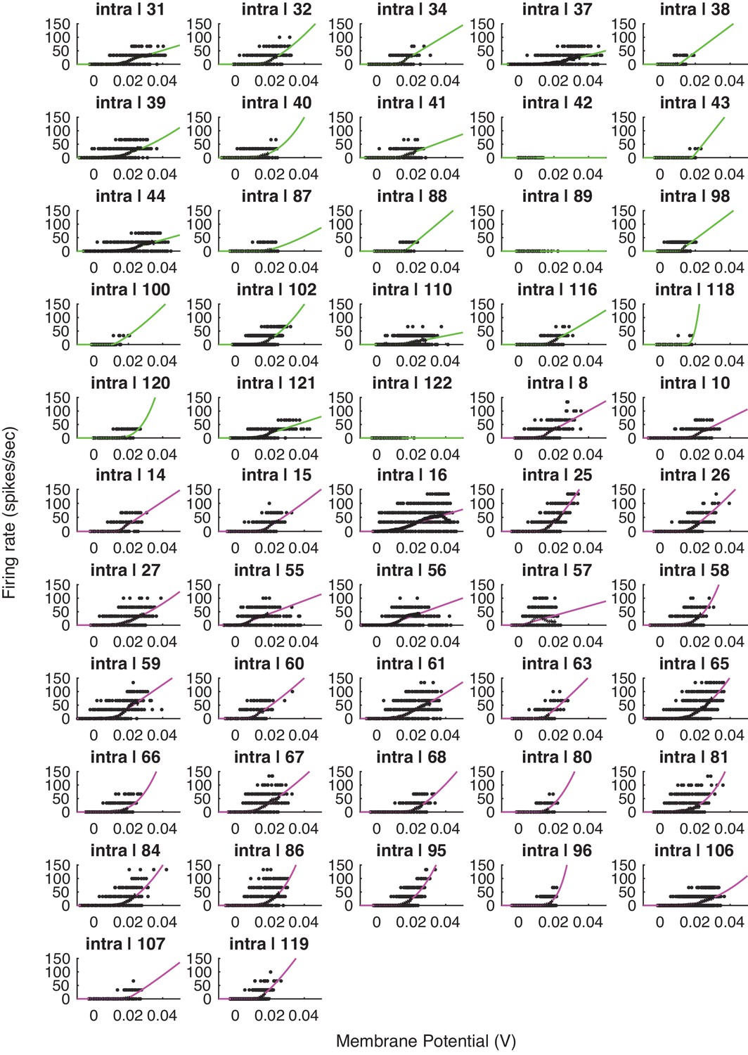
Voltage-to-firing rate transforms for all cells in the study.
This figure includes all cells, including cells that exhibited no 1 mV bin with at least 15 spikes (inclusion criteria for the group analysis).
Figure 7

Increases in membrane potential selectivity and input-output gain are both required for mature direction selectivity and firing rates.
(A) Actual mean spiking response rates for each stimulus plotted against the mean spiking response that is obtained by applying the voltage-to-firing rate transform to each stimulus’s membrane potential record for all naive cells (N = 16), showing that the phenomenological model captures the voltage-to-membrane transfer well. (B) Same, for experienced cells (N = 29). Model captures the actual spiking responses well. (C) Actual direction index values derived from the mean responses (F0) of naive and experienced cells. (D) Simulations of what we would expect if naive or experienced waveforms were paired with naive or experienced voltage-to-firing rate transforms. Plots show vertical histograms (with 5–95 percentile error bars) of mean direction selectivity index values for 10,000 simulations of 20 cells for several cases: 1) randomly selected naive voltage waveforms applied to randomly selected naive voltage-to-firing rate transforms; 2) randomly selected experienced voltage waveforms applied to randomly selected naive voltage-to-firing rate transforms; 3) randomly selected naive voltage waveforms applied to randomly selected experienced voltage-to-firing rate transforms, and 4) randomly selected experienced voltage waveforms applied to randomly selected experienced voltage-to-firing rate transforms. Scale bar on top of histogram shows 100 simulations. Axis labels identify the model by the waveforms used (top symbol) and voltage-to-firing rate transform used (bottom symbol). Actual data values are shown as dashed lines. To achieve increases in direction selectivity, it was only necessary for the model to adopt the voltage response waveforms of the experienced animals: the increased gain of the experienced animals was not necessary. (E+F) Same as C,D, but response to preferred direction is shown. Scale bar shows 50 simulations. To achieve increases in firing rates observed in experienced animals, experienced voltage-to-firing rate transforms were necessary. In D,F, models can be compared to whether they match the individual cell data by seeing if the individual cell data mean across cells falls within the 5–95%-tile range (the distribution of means is sampled empirically through simulation). Overall, to achieve both increases in direction selectivity and firing rate that are observed in vivo, changes in voltage responses and voltage-to-firing rate transform were necessary.
Tables
Key resources table
| Reagent type (species) or resource | Designation | Source or reference | Identifiers | Additional information |
|---|---|---|---|---|
| Software, algorithm | Matlab | The MathWorks, Natick, MA | RRID:SCR_001622 | |
| Software, algorithm | GitHub | GitHub | RRID:SCR_002630 | |
| Software, algorithm | Psychophysics Toolbox | Psychtoolbox.org | RRID:SCR_002881 | |
| Software, algorithm | Spike2 | Cambridge Electronic Design | ||
| Other | Spyder Express 3 | Datacolor | ||
| Strain, strain background (Mustela putorius furo) | Ferrets | Marshall Bio-resources | ‘Conventional’ colony | Females |
| Other | Electrode Puller | Sutter Instrument Company | P-97 with box filament | |
| Other | Micromanipulator | Sutter Instrument Company | MP-285 | |
| Other | Microelectrode amplifier | Axon Instruments (now Molecular Devices) | AxoClamp-2B | |
| Other | Multifunction data acquisition system | Cambridge Electronic Design | Micro1401 |
Additional files
Download links
A two-part list of links to download the article, or parts of the article, in various formats.
Downloads (link to download the article as PDF)
Open citations (links to open the citations from this article in various online reference manager services)
Cite this article (links to download the citations from this article in formats compatible with various reference manager tools)
Synaptic and intrinsic mechanisms underlying development of cortical direction selectivity
eLife 9:e58509.
https://doi.org/10.7554/eLife.58509


