Research Article

Nuclear crowding and nonlinear diffusion during interkinetic nuclear migration in the zebrafish retina

Department of Physiology, Development and Neuroscience, University of Cambridge, United Kingdom
Department of Applied Mathematics and Theoretical Physics, Centre for Mathematical Sciences, University of Cambridge, United Kingdom
Howard Hughes Medical Institute, Janelia Research Campus, United States

Oct 6, 2020

https://doi.org/10.7554/eLife.58635

Version of Record

Accepted for publication after peer review and revision.

Download
Cite
Share
CommentOpen annotations (there are currently 0 annotations on this page).

Version of Record published: October 6, 2020 (This version)
Accepted: September 3, 2020
Received: May 6, 2020

1. Of interest
The Slingshot phosphatase 2 is required for acrosome biogenesis during spermatogenesis in mice

Ke Xu, Xianwei Su ... Hongbin Liu

Research Article Updated Mar 31, 2023
Further reading

Article
Figures and data
Abstract
Introduction
Results
Discussion
Materials and methods
Appendix 1
Data availability
References
Decision letter
Author response
Article and author information
Metrics

Abstract

An important question in early neural development is the origin of stochastic nuclear movement between apical and basal surfaces of neuroepithelia during interkinetic nuclear migration. Tracking of nuclear subpopulations has shown evidence of diffusion - mean squared displacements growing linearly in time - and suggested crowding from cell division at the apical surface drives basalward motion. Yet, this hypothesis has not yet been tested, and the forces involved not quantified. We employ long-term, rapid light-sheet and two-photon imaging of early zebrafish retinogenesis to track entire populations of nuclei within the tissue. The time-varying concentration profiles show clear evidence of crowding as nuclei reach close-packing and are quantitatively described by a nonlinear diffusion model. Considerations of nuclear motion constrained inside the enveloping cell membrane show that concentration-dependent stochastic forces inside cells, compatible in magnitude to those found in cytoskeletal transport, can explain the observed magnitude of the diffusion constant.

Introduction

The vertebrate nervous system arises from a pseudostratified epithelium within which elongated proliferating cells contact both the apical and basal surfaces. Within these cells, striking nuclear movements take place during the proliferative phase of neural development. More than 80 years ago, these movements, termed interkinetic nuclear migration (IKNM), were shown to occur in synchrony with their cell cycle (Sauer, 1935). Under normal conditions, nuclei of proliferating cells undergo mitosis (M) exclusively at the apical surface. During the first gap phase (G1) of the cell cycle, nuclei migrate away from this surface to reach more basal positions by synthesis phase (S), when DNA is replicated. In the second gap phase (G2), nuclei migrate rapidly toward the apical surface where they divide again (Del Bene, 2011; Sauer, 1935; Baye and Link, 2007; Leung et al., 2011; Kosodo et al., 2011; Norden et al., 2009). The molecular mechanisms that drive the rapid nuclear movement in G2 have been investigated in a number of tissues (Norden, 2017). In the mammalian cortex, they are thought to involve microtubules, as well as various microtubule motors and actomyosin (Xie et al., 2007; Tsai et al., 2007), while in the zebrafish retina, it appears to be the actomyosin complex alone that moves the nuclei to the apical surface during G2 (Norden et al., 2009; Leung et al., 2011). Nuclear movements during the majority of the cell cycle, in G1 and S phases, have been less thoroughly examined. Although similar molecular motors have been implicated (Schenk et al., 2009; Tsai et al., 2010), the underlying molecular processes remain unclear.

Importantly, IKNM is known to affect morphogenesis and cell differentiation in neural tissues (Spear and Erickson, 2012), as retinas with perturbed IKNM are known to develop prematurely and to display abnormalities in cell composition (Del Bene et al., 2008). Given this regulatory involvement of IKNM in retinal cell differentiation, a deeper understanding of the nuclear movements remains a major prerequisite for insights into the development of neural systems. On a phenomenological level, studies tracking individual nuclei in the zebrafish retina during the G1 and S phases have shown their movement to resemble a stochastic process (Norden et al., 2009; Leung et al., 2011), particularly in the form of the mean squared nuclear displacement versus time. When these relations are linear or slightly convex, they indicate a random walk (or persistent random walk), much as in ordinary thermal diffusion. During these periods, individual nuclei switch between apical and basal movements at random intervals, leading to great variability in the maximum basal position they reach during each cell cycle (Baye and Link, 2007). Similarly, in the mammalian cerebral cortex, the considerable internuclear variability in IKNM leads to nuclear positions scattered throughout the entire neuroepithelium in S phase (Sidman et al., 1959; Kosodo et al., 2011). In addition to the stochastic movements of nuclei during IKNM, there is also a slow basalward drift of the entire population of nuclei. As variable basalward-biased migration was observed in nuclear-sized microbeads inserted in between cells during IKNM in the mouse cortex (Kosodo et al., 2011), it seems likely that passive forces are involved in this drift. A number of possible explanations for these passive processes have been put forward. These suggestions include the possibility of direct energy transfer from rapidly moving G2 nuclei (Norden et al., 2009), as well as nuclear movements caused by apical crowding (Kosodo et al., 2011; Okamoto et al., 2013), that is an increase in nuclear packing density close to the apical tissue surface. Here, we present experiments and theoretical analyses to test both hypotheses, particularly that of apical crowding, and to assess quantitatively whether active forces are also necessary for basal drift.

While a linear scaling of the mean squared displacement with time is a hallmark of diffusive processes, there is now growing evidence in disparate systems of dynamics that exhibit such scaling, yet are decidedly different from conventional diffusion in other respects (Wang et al., 2009; Leptos et al., 2009). Thus, a full test of the apical crowding hypothesis requires the study of the entire spatio-temporal distribution of nuclei within the retinal tissue. Our work relies on the tracks of closely packed nuclei of zebrafish retinal progenitor cells (RPCs). The retina of the oviparous zebrafish is easily accessible to light microscopy throughout embryonic development (Avanesov and Malicki, 2010) and has been used for several studies of the movements of nuclei during IKNM (Baye and Link, 2007; Del Bene et al., 2008; Norden et al., 2009; Sugiyama et al., 2009; Leung et al., 2011). We find evidence for IKNM being driven by apical crowding and further develop this idea into a mathematical model. Given the seemingly stochastic nature of individual nuclear trajectories, we base the model on a comparison between IKNM and a simple diffusion process. The model reveals the remarkable and largely overlooked importance of simple physical constraints imposed by the overall tissue architecture and allows us to describe accurately the global distribution of nuclei as a function of time within the retinal tissue. In this way, we describe IKNM as a tissue-wide rather than a single-cell phenomenon. We further develop the model by examining the motion of nuclei within the constrained environment of the enveloping cell membrane. This allows for an estimate of the hydrodynamic drag experienced by the nuclei, and hence of their diffusivity if the system were in thermodynamic equilibrium. We conclude from the magnitude of the diffusivity extracted from the data that basalward migration of nuclei during IKNM cannot be due to thermal diffusion alone. Instead, the model indicates that a stochastic force comparable with that which could be generated by cytoskeletal transport mechanisms must drive nuclear movements during IKNM. Finally, we obtain a mathematical description of the stochastic trajectories of individual nuclei in the presence of a finite concentration of others. Simulations of these trajectories also confirm that IKNM can only be understood when taking interactions between individual nuclei into account and hint at the way in which nuclei interact in a tissue-wide fashion. This description raises new questions about how cells sense and respond to being crowded, and may shed light on other aspects of progenitor cell biology, such as the statistics of cell cycle exit and cellular fate choice.

Results

Generating image sets with high temporal resolution

We imaged fluorescently labeled nuclei of whole retinas of developing zebrafish at 2 min intervals, an optimal time period given the difficulty to track nuclei accurately over long times and the increased photobleaching with shorter intervals. We compared movies of retinas imaged at 2 min and at 20 s intervals over a period of 2 hrs and found that the improvement in temporal resolution made no difference to our analyses. This suggests that it is unlikely that there are important intervening movements that might complicate the analysis within each 2-min interval.

To follow the nuclei of all cells within a portion of the retina, we used H2B-GFP transgenic lines with GFP expression exclusively in the nuclei (Figure 1A). In order to achieve the desired temporal resolution without sacrificing image quality, fluorescence bleaching and sample drift must be minimized as much as possible. The retinas of H2B-GFP embryos were imaged using either a single-angle lightsheet microscope (see Figure 1B for a schematic) or an upright two-photon scanning microscope. Both of these methods yield images with minimal bleaching compared to other microscopic techniques (Svoboda and Yasuda, 2006; Stelzer, 2015). However, while the single-angle lightsheet can generate large stacks of images, it is very sensitive to lateral drift due to a small area of high resolution imaging. Therefore, some data sets were produced using two-photon microscopy, which, despite the limitations of scanning time, could produce areas of high-resolution images of sufficient size.

Figure 1

Download asset Open asset

Imaging and tracking fluorescently labeled nuclei.

(A) A transgenic H2B-GFP embryonic retina imaged using lightsheet microscopy at ∼30 hpf. The lens, as well as apical and basal surfaces are indicated. (B) A schematic representation of single-angle lightsheet imaging of the retina. Laser light is focused into a sheet of light by the illumination objective and scans the retina. Fluorescent light is then collected by the perpendicular detection objective. (C) Track visualization and curation using the MaMuT plugin of Fiji. All tracks within a volume of the retina are curated and visualized. Circles and dots represent centers of nuclei, and lines show their immediate (10 previous steps) track. (D) The position of a single nucleus within the retinal tissue from its birth to its eventual division. The magenta dot indicates the nucleus tracked at various time points during its cell cycle. The last four panels are at shorter time intervals to highlight the rapid movement of the nucleus prior to mitosis.

Both lightsheet and two-photon microscopes produced images of at least half the retina with a depth of at least 50 μm over several hours in 2-min intervals. The images were processed using a suite of algorithms (Amat et al., 2015) to compress them to a lossless format, Keller Lab Block (KLB), correct global and local drift, and normalize signal intensities for further processing. Automated segmentation and tracking, in three dimensions, of the nuclei were carried out through a previously published computational pipeline that takes advantage of watershed techniques and persistence-based clustering (PBC) agglomeration to create segments and Gaussian mixture models with Bayesian inference to generate tracks of nuclei through time (Amat et al., 2014). Two main parameters greatly affect tracking results, overall background threshold and PBC agglomeration threshold. To obtain best automated tracking results, ground truth tracks were created for a section of the retina over 120 min and were compared to tracks generated over a range of these two parameters. The best combination of the two parameters was chosen as the one with highest tracking fidelity and lowest amount of oversegmentation in that interval.

The most optimal combination of parameters yielded an average linkage accuracy, from each time point to the next, of approximately 65%. Hence, extensive manual curation and correction of tracks were required. Tracking by Gaussian mixture models (TGMM) software generates tracks that can be viewed and modified using the Massive Multi-view Tracker (MaMuT) plugin of the Fiji software (Wolff et al., 2018; Schindelin et al., 2012). A region of the retina with the best fluorescence signal was chosen and all tracks within that region were examined and any errors were corrected. The tracks consist of sequentially connected sets of 3D coordinates representing the centers of each nucleus (Figure 1C), with which their movement across the tissue can be mapped over time. For example, Figure 1D shows IKNM of a single nucleus tracked from its birth, at the apical surface of the retina, to its eventual division into two daughter cells.

Analysis of nuclear tracks

This process yielded tracks for hundreds of nuclei, across various samples, over time intervals of at least 200 min. We used custom-written MATLAB scripts to analyze these tracks. The aggregated tracks of the main data set, in Cartesian coordinates, for all tracked lineages are shown in Figure 2A. Single tracks for any given time interval can be extracted and analyzed from this collection. In order to transform the Cartesian coordinates of the tracks into an apicobasal coordinate system, we drew contour curves at the apical surface of the retina (see Figure 1A) separating RPC nuclei from the elongated nuclei of the pigmented epithelium. We then calculated curves of best fit (second degree polynomials) in both the XY and YZ planes. Assuming that the apical cortex is perpendicular to the apicobasal axis of each cell, displacement vectors of the nuclei at each time point can be separated into apicobasal and lateral components. Since, in IKNM, the apicobasal motion is that of interest, we used this component for our remaining analyses.

Figure 2

Download asset Open asset

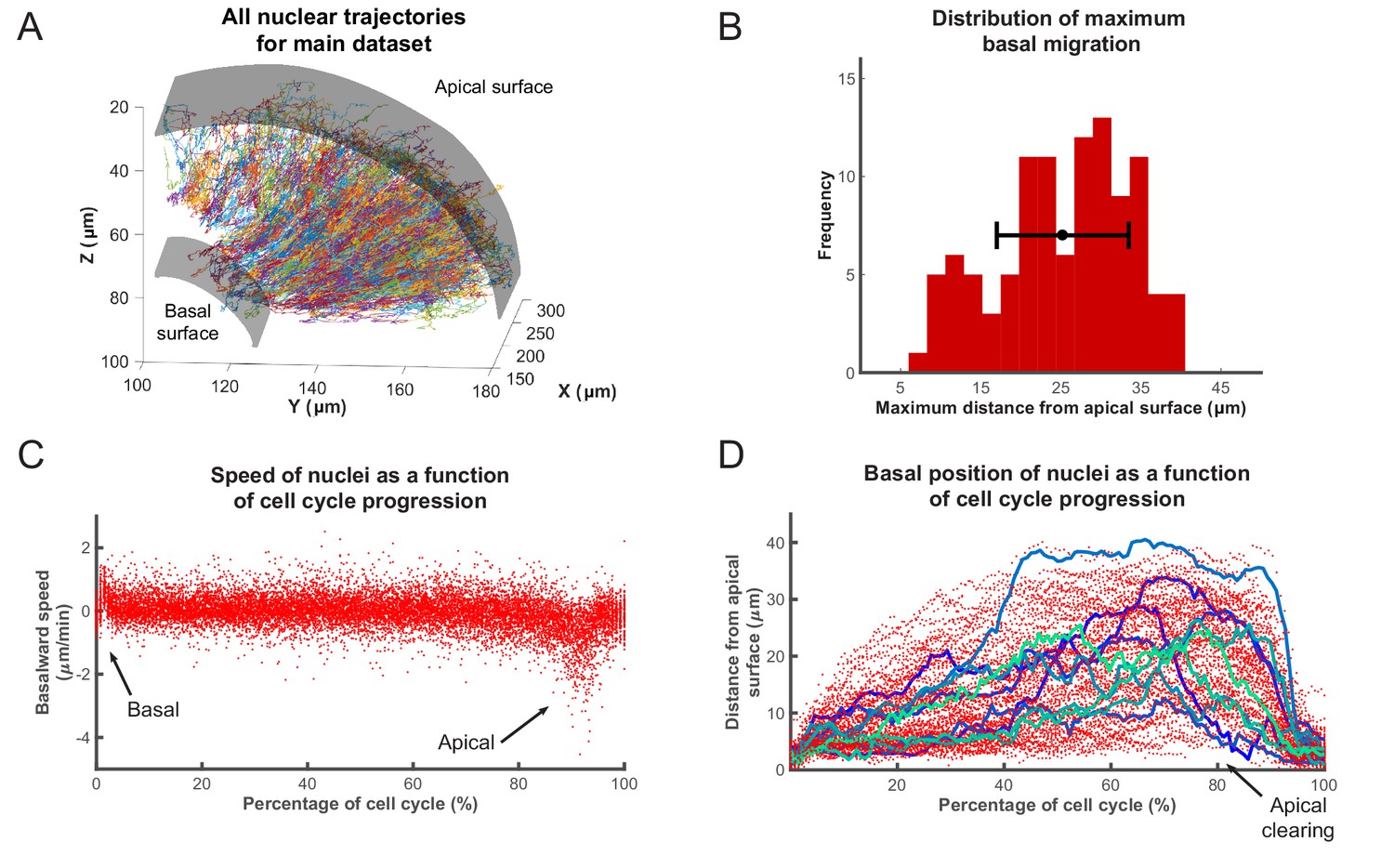
Analysis of nuclear tracks during IKNM.

(A) Extracted trajectories of nuclei in three dimensions. All curated tracks of the main data set over 400 min in the region shown in Figure 1C are presented. (B) The distribution of maximum distances reached away from the apical surface by nuclei during their completed cell cycles. The mean and one standard deviation are shown. (C) The speed distribution of 106 nuclei over complete cell cycles. The cell cycle lengths of all nuclei were normalized and superimposed to highlight the early basal burst of speed, as well as pre-division apical rapid migration. The speeds between these two periods are normally distributed. (D) Position of the same nuclei as in (C) measured by their distance from the apical surface over normalized cell cycle time. Even though all nuclei start and end their cell cycle near the apical surface, they move out across the retina to take positions in all available spaces, creating an apical clearing as indicated. Tracks for 10 randomly chosen nuclei are shown as colored lines to highlight the variability in the traversed trajectories.

Figure 2C,D show the speed and position of tracked nuclei of the same data set, over the duration of their cell cycle, for all cells that went through a full cell cycle. While all nuclei behave similarly minutes after their birth (early G1) and before their division (G2), their speed of movement and displacement is highly variable for the majority of the time that they spend in the cell cycle (Figure 2C,D). Most daughter nuclei move away from the apical surface, within minutes of being born, with a clear basalward bias in their speed distribution (Figure 2C). This abrupt basal motion of newly divided nuclei has also been recently observed by others (Leung et al., 2011; Shinoda et al., 2018; Barrasso et al., 2018). However, immediately after this brief period, nuclear speeds become much more equally distributed between basalward and apicalward, with a mean value near 0. Such a distribution is indicative of random, stochastic motion, which in turn leads to a large variability in the position of nuclei within the tissue (away from the apical surface) during the cell cycle (Figure 2B).

Interestingly, except during mitosis, we find an apical clearing of a few microns for dividing cells (Figure 2D). We checked to see if this was an artifact of measuring the distance to nuclear centers due to nuclear shape, as nuclei are rounded during M phase but are more elongated along the apicobasal axis at other times. We found no significant difference between the average length of the nuclear long axis when measured for 50 random nuclei right before their division (5.0 ± 0.7 µm) compared to 50 others chosen randomly from any other time point within the cell cycle (5.3 ± 1.1 µm), indicating that this clearing is likely to have a biological explanation, such as the preferential occupancy of M phase nuclei and surrounding cytoplasm at the apical surface during IKNM. We also performed the same measurements for 25 random nuclei 10 min after division when the average long axis length is significantly decreased by 0.8 fold (3.9 ± 0.5 µm). However, this measurement increased significantly in the following 10 min (4.8 ± 0.7 µm) to become similar to that at M phase.

Basal movement of nuclei is driven like a diffusive process

Previous work has shown that when RPCs are pharmacologically inhibited from replicating their DNA, their nuclei neither enter G2 nor exhibit rapid persistent apical migration that normally occurs during the G2 phase of the cell cycle (Leung et al., 2011; Kosodo et al., 2011). A more surprising result of these experiments is that the stochastic movements of nuclei in G1 and S phases also slow down considerably during such treatment (Leung et al., 2011). It was, therefore, suspected that the migration of nuclei of cells in G2 toward the apical surface jostles those in other phases (Norden et al., 2009). We searched our tracks for evidence of such direct kinetic interactions among nuclei by correlating the speed and direction of movement of single nuclei with their nearest neighbors. These neighbors were chosen such that their centers fell within a cylindrical volume of a height and base diameter twice the length of long and short axes, respectively, of an average nucleus. Figure 3A shows the lack of correlation between the speed of movement of nuclei and the average speed of their neighbors. We further categorized the neighboring nuclei by their position in relation to the nucleus of interest (along the apicobasal axis), their direction of movement, and whether they were moving in the same direction of the nucleus of interest or not. None of the resulting eight categories of neighboring nuclei showed a correlation in their average speed with the speed of the nucleus of interest. Furthermore, we considered the movement of neighboring nuclei one time point (2 min) before or one time point after the movement of the nucleus of interest. Yet, we still found no correlation between these time-delayed and original speeds. These results suggest that there does not appear to be much transfer of kinetic energy between neighboring nuclei, and this is consistent with general considerations of the strongly overdamped character of motion at these length scales.

Figure 3

Download asset Open asset

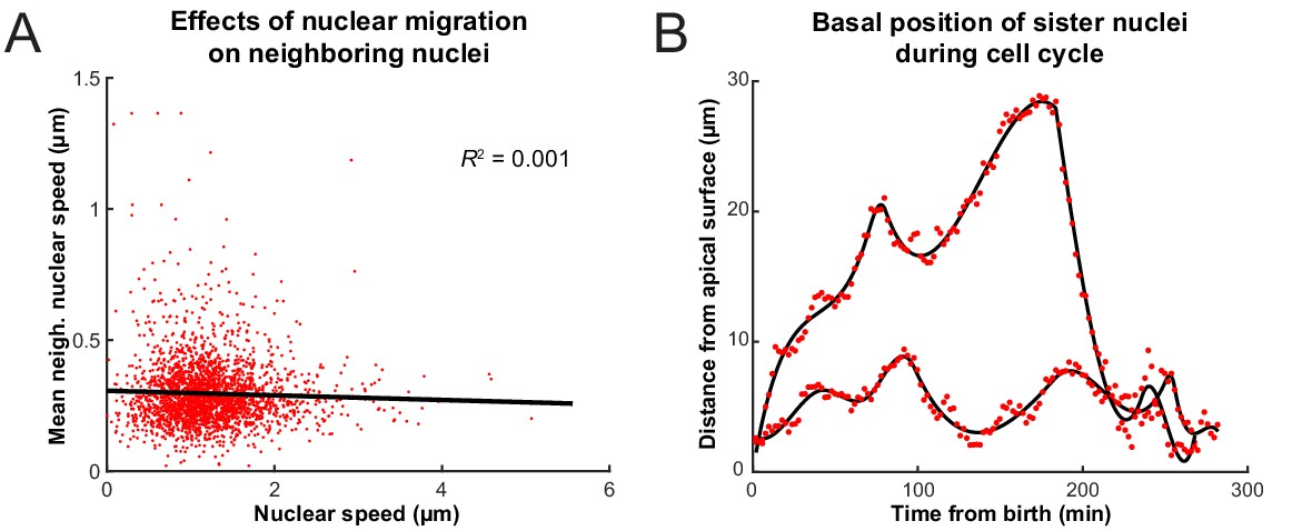
Interactions of nuclei in close proximity.

(A) Average speed of nuclei neighboring a nucleus of interest as a function of the speed of that nucleus. (B) The positions of two sister nuclei at each time point imaged (red circles) over their complete cell cycle. The black lines are spline curves indicating the general trend of their movements.

Another hypothesis advanced for the basal drift in IKNM is that the nuclear movements are driven by apical crowding (Kosodo et al., 2011; Okamoto et al., 2013). How apical crowding might result in basal IKNM can be understood by comparing IKNM to a diffusive process. In diffusion, a concentration gradient drives the average movement of particles from areas of high to areas of low concentration. However, despite the average movement being directed, each individual particle’s trajectory is a random walk (Reif, 1965). Similarly, during IKNM a gradient in nuclear concentration is generated because nuclei divide exclusively at the apical surface. If basal IKNM were comparable to diffusion, this nuclear concentration gradient would be expected to result in a net movement of nuclei away from the area of high nuclear crowding at the apical side of the neuroepithelium (Miyata et al., 2014; Okamoto et al., 2013). Indeed, in IKNM each individual nucleus’ trajectory resembles a random walk (Norden et al., 2009). Therefore, for the cells in the G1 and S phases (which account for more than 90% of the cell cycle time in our system), IKNM has, at least on a phenomenological level, the main features of a diffusive process.

To test further whether we can indeed describe IKNM using a model of diffusion, we first asked what would happen to the concentration gradient if we blocked the cell cycle in S phase, which inhibits both the apical movement of the nuclei in G2 and mitosis at the apical surface. If the comparison to diffusion were valid, we expect the blockage to abolish the build-up and maintenance of the concentration gradient. We, therefore, compared the normally evolving distribution of nuclei in a control retina with that measured from a retina where the cell cycle was arrested at S phase using a combination of hydroxyurea (HU) and aphidicolin (AC) (Leung et al., 2011; Icha et al., 2016). These compounds inhibit DNA polymerase and ribonuclear reductase, respectively, to halt DNA replication (Baranovskiy et al., 2014; Singh and Xu, 2016). In the HU-AC-treated retina, we counted the number of nuclei in a three-dimensional section of the tissue containing approximately 100 nuclei, at equal time intervals, starting with 120 min after drug treatment. The delay ensured that almost all cell divisions, from nuclei that had already completed the S phase at the time of treatment, had taken place. These results are shown in Figure 4A,C, in which retinal tissue is approximated as a spherical shell of apical radius a and the rescaled coordinate $ξ = r / a$ , where r is the distance from the center of the lens, is presented on the x-axis. As expected from the diffusion model (Figure 4D), over the course of 160 min, the mean of the nuclear distribution moved further toward the basal surface in treated retinas, and the concentration difference between the apical and basal surfaces diminished (Figure 4B,C). In contrast, in control retinas the mean of the nuclear distribution moved toward the apical surface (Figure 4A,C) as the gradient continued to build up. Hence, these results support the suitability of a diffusive model to describe the basal nuclear migration during IKNM.

Figure 4

Download asset Open asset

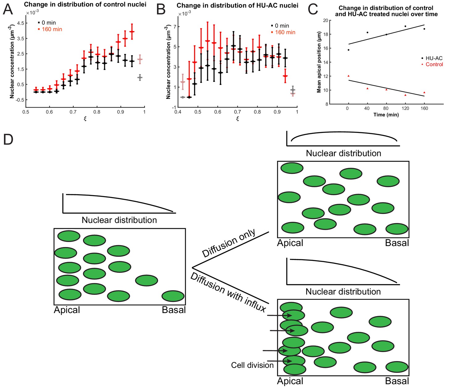
Nuclear concentration gradient across the apicobasal axis of the retina.

The concentration of nuclei is higher near the apical surface compared to the basal surface. (A) In the control retina, the nuclear concentration gradient builds up over time. (B) Blocking apical migration and division of nuclei, by inhibiting S phase progression, leads to a shift in the distribution of nuclei toward the basal surface in the HU-AC treated retina. In A and B, the coordinate $ξ = r / a$ is used, where a is the radius of the apical surface and r the distance from the center of the lens. (C) The shift in the distribution of nuclei under HU-AC treatment when compared to the untreated retina. The average distance of nuclei away from the apical surface increases consistently over time in the absence of cell division, but remains the same when new nuclei are constantly added at the apical surface. (D) A schematic of how a diffusion model would work in the context of IKNM in the retina. A concentration gradient of nuclei (left) would drive the net movement of nuclei from the apical surface to the basal surface. However, without maintenance of the gradient, the drive for this net migration is lost (top right). In the retina, the gradient is maintained through cell divisions at the apical surface, modeled as a one-way influx across the apical surface (bottom right), continuously driving the net movement basally.

An analytical diffusion model of IKNM

To investigate whether a diffusion model provides a quantitative description of IKNM, we focused on the crowding of nuclei at the apical side of the tissue. In mathematical terms, crowding creates a gradient in nuclear concentration c along the apicobasal direction of the retina. If we assume there is no dependence of the nuclear concentration on the lateral position within the tissue then we require a diffusion equation for the nuclear concentration $c (r, t)$ as a function only of the apicobasal distance r and time t. The retina can be approximated as one half of a spherical shell around the lens, and thus we use spherical polar coordinates with the origin of the coordinate system at the center of the lens, the basal surface at $r = b$ and the apical surface at $r = a$ (Figure 5B). We first consider the simplest diffusion equation for this system, in which there is a diffusion constant D independent of position, time, and c itself, namely

\frac{\partial c}{\partial t} = \frac{D}{r^{2}} \frac{\partial}{\partial r} (r^{2} \frac{\partial c}{\partial r}) .

Figure 5

Download asset Open asset

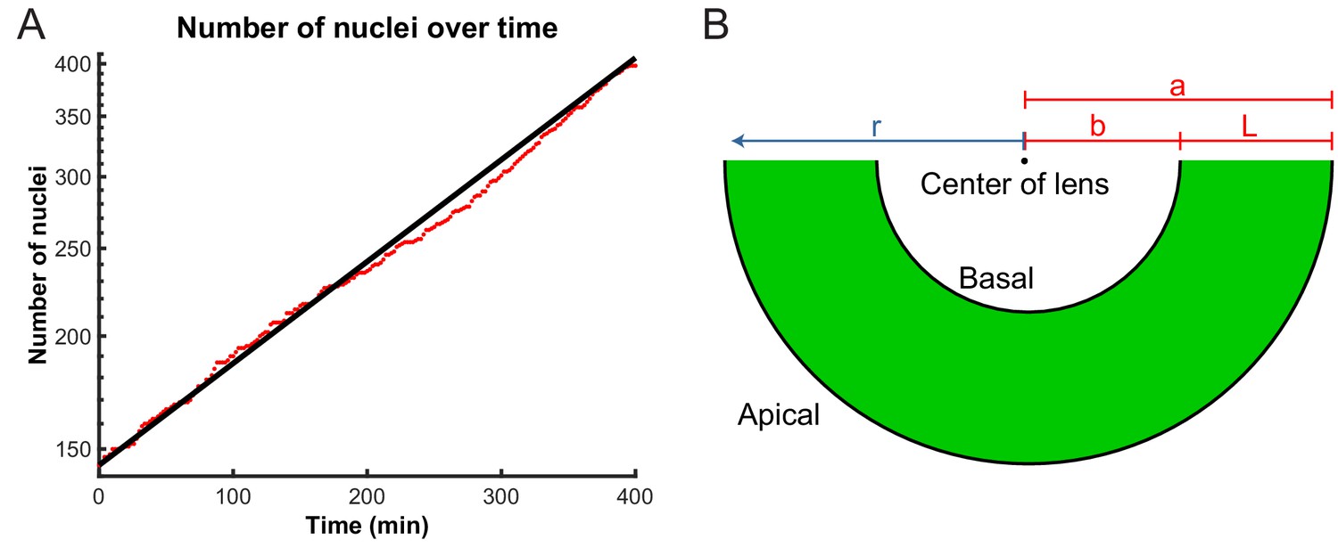
Model parameters extracted from experimental data.

(A) Number of nuclei grows exponentially during the proliferative stage of the retinal development. A line can be fitted to the log-lin graph of nuclear numbers as a function of time to extract the doubling time (cell cycle length) in this period. (B) A schematic of the retina indicating the variables used in the diffusion model of IKNM. a: distance from center of lens to apical surface; b: distance from center of lens to basal surface; L: thickness of the retina; r: distance from center of lens for each particle.

We seek to determine D from the experimental data of the concentration profile $c (r, t)$ . Note that in this parsimonious view of modeling we have not included a ‘drift’ term of the kind that is expected to be present at the very late stages of IKNM, when nuclei return to the apical side.

In addition to Equation 1, we must specify the boundary conditions appropriate to IKNM. Since nuclei only divide close to the apical surface of the tissue, we treat mitosis as creating an effective influx of nuclei through the apical boundary. To quantify this influx, we extracted the number of cells $N (t)$ as a function of time. As during the stages of development examined here cells are neither dying nor exiting the cell cycle (Biehlmaier et al., 2001), we assumed that the number of cell divisions is always proportional to the number of currently existing cells. This assumption predicts an exponential increase in the number of cells or nuclei, over time, as was recently confirmed by Matejčić et al., 2018:

N (t) = N_{0} e^{t / τ},

where $N_{0}$ is the initial number of nuclei and $τ = T_{P} / \ln 2$ , with $T_{P}$ the average cell cycle length. Figure 5A shows the agreement between the theoretically predicted curve $N (t)$ with the experimentally obtained numbers of nuclei over time. Having obtained $N_{0}$ and $T_{P}$ from our experimental data, the predicted curve has no remaining free parameters and thus no fitting is necessary. Using Equation 2, we formulate the influx boundary condition as

{D \frac{\partial c}{\partial r} |}_{r = a} = \frac{1}{S} \frac{\partial N (t)}{\partial t} = \frac{N_{0}}{S τ} e^{t / τ},

with S the apical surface area of our domain of interest. In contrast to the apical side of the tissue, there is no creation (or depletion) of nuclei at the basal side (Matejčić et al., 2018), and hence a no-flux boundary condition,

{\frac{\partial c}{\partial r} |}_{r = b} = 0.

The position $r = b$ where this basal boundary condition is applied could change throughout tissue development. Matejčić et al., 2018 found that a basal exclusion zone, where nuclei cannot enter due to accumulation of basal actin, exists in the zebrafish retina before approximately 42 hpf. Before this point in development, the no-flux boundary condition is applied at the tissue radius where the nuclear exclusion zone begins, while later in development, the no-flux boundary condition should be applied at the position of the actual basal cell surfaces. Here, we only model early stages of embryonic development well before the disappearance of the basal exclusion zone, therefore the location $r = b$ , where we apply our basal boundary condition, is chosen such that we only consider the region of the retinal tissue actually accessible to moving nuclei during IKNM. Thus, taken together, Equations 1, 3 and 4 fully specify this simplest mathematical model of IKNM.

In solving these equations to find the concentration of nuclei $c (r, t)$ in the retinal tissue it is convenient to introduce dimensionless variables for space and time,

ξ = \frac{r}{a}, s = \frac{D t}{a^{2}},

and further define the purely geometric parameter $ρ = b / a < 1$ . The exact solution for the nuclear concentration, whose detailed derivation is given in the Appendix, is

c (ξ, s) = \sum_{i = 1}^{\infty} (h_{i} e^{- λ_{i}^{2} s} + \frac{α_{i} f_{0}}{σ + λ_{i}^{2}} e^{σ s}) H_{i} (ξ) + \frac{1}{1 - ρ} (\frac{1}{2} ξ^{2} - ρ ξ + g_{0}) f_{0} e^{σ s} .

The first terms within parentheses describe the decay over time of the initial condition $c (ξ, s = 0)$ . Here, $λ_{i}$ are the eigenvalues and $H_{i} (ξ)$ the eigenfunctions of the radial diffusion problem, and the coefficients $h_{i}$ are determined from the experimental initial conditions (see Materials and methods). The second terms within the sum and the final term on the right hand side of Equation 6 are constructed such that the solution fulfills the boundary conditions Equation 3 and Equation 4. In the last term, the constant $g_{0}$ was obtained using the constraint that the volume integral of the initial concentration yields the initial number of nuclei $N_{0}$ . $f_{0}$ , σ and $α_{i}$ emerge within the calculation of the solution and are specified in the Appendix. Thus, the diffusion constant D in Equations 1 and 6 is the only unknown.

The linear model is accurate at early times

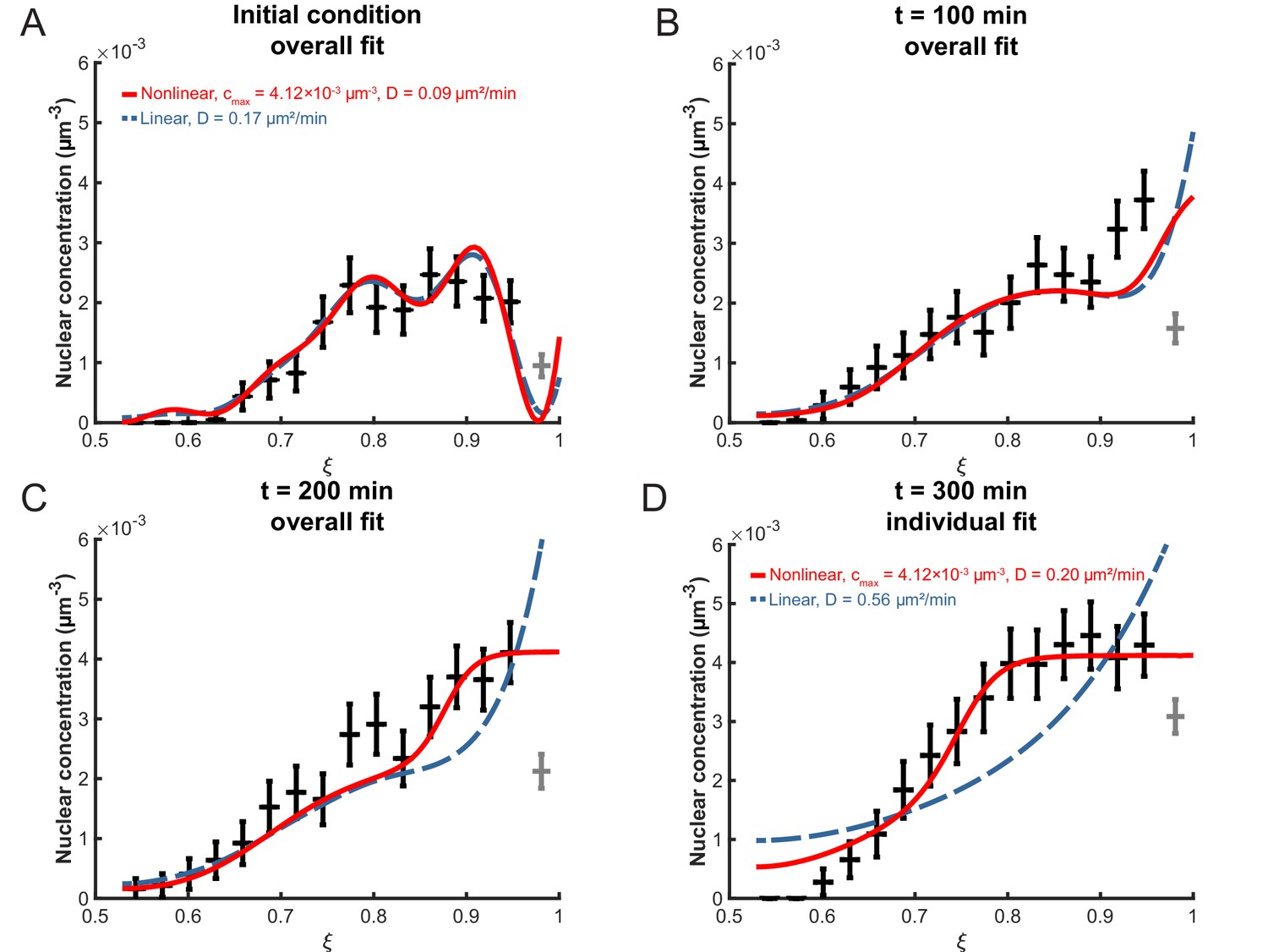
To determine the effective diffusion constant D from the data, the experimental distribution of nuclei in the retinal tissue was first converted into a concentration profile. Then, the optimal D-value, henceforth termed $D^{*}$ , was obtained using a minimal- $χ^{2}$ approach. The value obtained within the linear model for a binning width of 3 μm and an apical exclusion width of 4 µm is $D_{lin}^{*} = 0.17 \pm 0.07$ µm²/min. Using this, we can examine the decay times of the different modes in the first term of Equation 6. The slowest decaying modes are the ones with the smallest eigenvalues $λ_{i}$ and we find that the longest three decay times are $𝒯_{1} \approx 1325$ min, $𝒯_{2} \approx 350$ min and $𝒯_{3} \approx 158$ min. This shows that indeed all three terms of Equation 6 are relevant on the timescale of our experiment and need to be taken into account when calculating the concentration profile. The corresponding plots of $c (ξ, s)$ are shown in Figure 6A–C. As can be seen from this figure, the diffusion model fits the data very well at early times, $t \leq 200$ min after the start of the experiment at 24 hpf (see Materials and methods). However, for $t \geq 200$ min the model does not fit the data as well; the experimentally observed nuclear concentration levels off at a value between $4.00 \times 10^{- 3}$ µm⁻³ and $4.50 \times 10^{- 3}$ µm⁻³ (Figure 6D), an aspect that is not captured by this model of linear diffusion.

Figure 6

Download asset Open asset

Fitting the linear and nonlinear models to the distribution of nuclei over time.

(A) The initial experimental concentration profile of nuclei at $t = 0$ min, as well as the calculated initial condition curves (see Materials and methods Equation 17) for the linear (red solid line) and nonlinear (blue dashed line) models. The fit of the models to experimental distribution of nuclei after 100 min (B), 200 min (C), and 300 min (D) are shown. For the first three graphs, the best fits over all 100 intervening time points were used with the corresponding diffusion constants shown in (A). For t = 300 min, the best fits at that time point only were used with the corresponding diffusion constants indicated.

One particular aspect of the biology that the linear model neglects is the spatial extent of the nuclei. In the linear diffusion model, particles are treated as point-like and non-interacting. However, our microscopy images (see Figure 1A) clearly indicate that the nuclei have finite incompressible volumes, so that their dense arrangement within the retinal tissue would lead to steric interactions once the nuclear concentration is sufficiently high. Moreover, the packing density of nuclei can not exceed a maximum value dictated by their geometry. Therefore, we next examined whether accounting for such volume and packing density effects leads to a more accurate theory describing the nuclear distribution during IKNM.

Nonlinear extension to the model

When the diffusion Equation 1 is written in the following form

\frac{\partial c}{\partial t} = D \frac{1}{r^{2}} \frac{\partial}{\partial r} {r^{2} c \frac{\partial}{\partial r} [\frac{\partial}{\partial c} (c \ln c)]},

we can identify the term $c \ln c$ as proportional to the entropy density $𝒮$ of an ideal gas, and its derivative with respect to c as a chemical potential. In an ideal gas, all particles are treated as point-like and without mutual interactions. In order to include the spatial extent of particles (i.e. the spatial extent of nuclei in this case), we must estimate the entropy in a way that accounts for the maximum concentration allowable given steric interactions. This is a well-studied problem in equilibrium statistical physics, in which, purely as a calculation tool, it is useful to consider space as divided up into a lattice of sites. Each of these sites can be either empty or occupied by a single particle. In this ‘lattice gas’ model, the discrete sites assure a minimum distance of approach for particles and thus effectively introduce a particle size and, correspondingly, a maximum particle concentration $c_{max}$ (Huang, 1987). In this system, a useful approximation to the entropy is

𝒮_{lattice gas} \propto c \ln c + (c_{max} - c) \ln (c_{max} - c) .

Substituting this expression for the term $c \ln c$ in Equation 7, we obtain the nonlinear diffusion equation

\frac{\partial c}{\partial t} = D \frac{1}{r^{2}} \frac{\partial}{\partial r} (r^{2} \frac{c_{max}}{c_{max} - c} \frac{\partial c}{\partial r}) .

The term 'nonlinear' refers to the mathematical structure of the newly obtained Equation 9. In the mathematical classification, an equation is linear in a certain variable if this variable only appears raised to the power one within the equation. For example, the simplest diffusion Equation 1 is linear in c and all its derivatives with respect to r and t, such as $\partial c / \partial t$ . In contrast, in Equation 9 the term $c_{max} / (c_{max} - c)$ appears which is proportional to $c^{- 1}$ . Hence, Equation 9 is said to be nonlinear. The additional nonlinear term in Equation 9 (as compared to Equation 1) is an important aspect of the model as it arose from the introduction of the spatial extent of the nuclei and their maximum possible packing density $c_{max}$ . This effect also has to be taken into account in the boundary conditions. Adjusting the boundary conditions at the apical side accordingly leads to

{D \frac{c_{max}}{c_{max} - c} \frac{\partial c}{\partial r} |}_{r = a} = \frac{N_{0}}{S τ} e^{t / τ},

while the basal boundary condition remains the same as Equation 4. Together, Equation 9 and the boundary conditions in Equations 4 and 10 represent an extension to the diffusion model for IKNM, which now accounts for steric interactions between the nuclei. The maximum concentration $c_{max}$ incorporated in this model was obtained, as described in the Materials and methods, by considering a range of nuclear radii and the maximum possible packing density for aligned ellipsoids (Donev et al., 2004).

Similar to fitting the linear model, we also need to establish a description of the initial condition. To make both models consistent with each other, we employ the linear model’s initial condition, Equation 6 at $s = 0$ with $h_{i}$ as obtained from Equation 17 (Figure 6A). The concentration profile in the nonlinear model and its derivative were obtained numerically using the MATLAB pdepe solver. Fitting this concentration profile to the data was by means of a minimal- $χ^{2}$ approach as well. When the optimization takes data points up to $t = 200$ min into account, we find $D_{nonlin}^{*} = 0.09 \pm 0.05$ µm²/min (Figure 6, Table 1). As can be seen, by choosing $c_{max}$ correctly, an excellent fit to the data can be obtained, particularly to the flattened part of the distribution at later times near the apical side ( $ξ \sim 1$ ), where the linear model fails. These results show that a lattice-gas based diffusion model is indeed suitable to describe time evolution of the nuclear concentration profile of the zebrafish retina during IKNM over several hours of early development.

Table 1

List of best-fit diffusion constants $D^{*}$ , their standard deviations and probabilities for the studied conditions.

	$D_{nonlin}^{*}$ (µm²/min)	$σ_{D}$ (µm²/min)	$P_{χ} (χ^{2}; ν)$
Normal	0.09	0.05	0.49–0.51
Normal (repeat sample)	0.10	0.06	0.47–0.48
High T	0.13	0.08	0.42
Low T	0.06	0.05	0.69–0.7

Basalward IKNM is not due to thermal diffusion but is compatible with cytoskeletal transport

This diffusion model, with the calculated diffusion constant $D_{nonlin}^{*} = 0.09 \pm 0.05$ µm²/min obtained from the nonlinear implementation, allows us to probe the physical and biological considerations that could set its scale. Notably, at low nuclear densities, $c ≪ c_{max}$ , the term $c_{max} / (c_{max} - c)$ in Equation 9 tends to unity, and the ordinary diffusion Equation 1 with $D_{lin}^{*} = D_{nonlin}^{*}$ is recovered. We can thus make use of its well-known properties for further evaluation. First, we assess whether nuclei in IKNM move due to free equilibrium thermal diffusion in a fluid. If so, the diffusion constant obeys the Stokes-Einstein equation (Einstein, 1905)

D_{thermal} = \frac{k_{B} T}{ζ},

where $k_{B} = 1.38 \times 10^{- 23}$ JK⁻¹ is the Boltzmann constant, T is the absolute temperature, and ζ is the drag coefficient for the particle, the constant of proportionality between the speed with which it moves and the force applied. For a spherical particle of radius $R$ in a fluid of viscosity η, the reference value is $ζ_{0} = 6 π η R$ . If we assume that the particles move in water at 25 °C, for which $η \approx 9 \times 10^{- 4}$ Pas, and if we approximate the nuclei as spheres with $R = 3.5$ µm, corresponding to the maximum nuclear concentration $c_{max} = 4.12 \times 10^{- 3}$ µm⁻³ (as in Figure 6), we obtain $D_{thermal} \approx 4.2$ µm²/min. This value is about 50 times larger than the measured value of $D_{nonlin}^{*}$ , implying that freely diffusing nuclei in water would be vastly more mobile than seen during IKNM.

While the free thermal diffusivity of nuclei serves as a useful reference quantity, nuclei clearly do not move in pure water, nor in an unbounded fluid. The viscosity of the cytoplasm is likely much higher than that of water due to the high number of organelles and polymeric components present; a higher viscosity leads to a lower diffusion constant via the Stokes-Einstein relation (Equation 11). Similarly, the slender shape of the individual cells within pseudostratified epithelia (Norden, 2017) would imply that a considerable amount of energy is required to transport fluid through the narrow region between the nucleus and the membrane.

In order to understand the effects of membrane confinement on fluid transport, it is useful to consider a minimal energetic description of the cell shape. That is provided by an energy $ℰ$ that incorporates membrane elasticity, through a bending modulus κ, and surface tension γ,

ℰ = \int 𝑑 S {\frac{κ}{2} ℋ^{2} + γ},

where $d S$ is the element of surface area and $ℋ$ is the mean curvature. For a cylindrically symmetric shape given by a function $δ (z)$ , $d S = 2 π δ \sqrt{1 + δ_{z}^{2}}$ and

ℋ = \frac{δ_{z z}}{{(1 + δ_{z}^{2})}^{3 / 2}} - \frac{1}{δ \sqrt{1 + δ_{z}^{2}}},

where $δ_{z}$ stands for $d δ / d z$ , etc. The equilibrium shape of a membrane is that which minimizes Equation 13 subject to constraints such as boundary conditions and/or a given enclosed volume.

As first understood in the context of the so-called ‘pearling instability’ of membranes under externally imposed tension (Bar-Ziv and Moses, 1994; Nelson et al., 1995; Goldstein et al., 1996), narrow necks emerge as characteristic equilibrium structures when the dimensionless ratio $γ R_{\infty}^{2} / κ$ is much larger than unity, where $R_{\infty}$ is a characteristic tube radius imposed far from the neck (e.g. the nuclear radius $R$ ). In this limit, the neck radius is on the order of $\sqrt{κ / γ}$ . For fluid membranes, it is known that $κ \sim 20 k_{B} T$ (Helfrich, 1973), while the magnitude of tension (an energy per unit area) is such that the surface energy associated with a molecular area is comparable to thermal energy; $γ ℓ^{2} / k_{B} T \sim 1$ , where $ℓ$ is a molecular dimension (e.g. 1 nm). Thus, γ may be as large as $\sim 10^{- 5}$ Jm⁻² and $γ R^{2} / κ$ is very large indeed ( $\sim 10^{5}$ ).

To illustrate the kinds of shapes that are energetic minima of Equation 12, we show in Figure 7 that which arises when we impose (i) an overall aspect ratio of $\sim 20$ for the cell, as measured by Matejčić et al., 2018, (ii) cell radii of 1.98 and 0.94 µm at the apical and basal sides of the tissue, respectively, as determined from that aspect ratio and the approximate length L of cells in our experiment, and (iii) position of the nucleus at the midpoint of the cell, with a radius $R = 3.5$ µm. The details of calculations are given in the Appendix. As the necks become extremely narrow in the relevant limit, we have taken a smaller value of γ to illustrate the basic effect. Because the gap between the membrane and the enveloped sphere is so thin, we have set the membrane radius equal to that of a sphere with membrane radius $R_{t u b e}$ over some angular extent and minimized the energy with respect to the position of the last contact point, as detailed in the Appendix.

Figure 7

Download asset Open asset

Cell shapes.

(A) Equilibrium cell shape obtained from minimization of elastic energy, with specified radii $δ_{a} = 1.98$ µm and $δ_{b} = 0.94$ µm at apical and basal sides. Here, the length L of the cell is taken to be 55 µm. (B) Coordinate system defined in Daniels, 2019, where $R$ is the nuclear radius and $R_{tube}$ and θ are the radius of the membrane tube around the nucleus and the opening angle of the membrane, respectively.

The similarity of this shape to those described in the literature suggests that this model is a useful starting point for the discussion of the fluid dynamics of nuclear motion during IKNM. Recently, Daniels, 2019 considered the transport of a sphere through the fluid contained within a cylindrically symmetric tight-fitting tubular membrane with bending modulus κ and surface tension γ, much like the geometry of cells undergoing IKNM. At a finite temperature T, the membrane will exhibit thermally driven shape fluctuations which, as shown by Helfrich, 1978, produce a repulsive interaction with the nearby sphere, swelling the gap. In the limit of large tension (appropriate for a tight-fitting membrane), the calculation simplifies to yield the result

ζ_{tube} = 32 ζ_{0} {(\frac{κ}{k_{B} T} \frac{γ R^{2}}{k_{B} T})}^{2 / 3},

where, for ease of interpretation, we have written the factors within parentheses as a product of two convenient dimensionless ratios. As the nuclear radius is micron-sized, we find $γ R^{2} / k_{B} T \sim 10^{7}$ , which in turn implies a drag coefficient ratio on the order of 10⁵ and diffusivities $D_{tube} \approx (1 - 5) \times 10^{- 6} D_{thermal}$ . Because of the very close spacing between the membrane and nucleus and the high viscous drag associated with such a geometry, these values are about 3 to 4 orders of magnitude smaller than the measured $D_{nonlin}^{*}$ . This is without considering changes in the cytoplasmic viscosity, which would decrease the value of D even further. Therefore, we conclude that the nuclear movements in IKNM cannot be due to thermal diffusion, but must be actively driven, for example through cytoskeletal transport.

We can turn to a more microscopic interpretation of the value of the diffusion constant. At low nuclear concentrations, when Equation 1 holds, the behavior of individual particles can be described using the overdamped Langevin equation (compare to Lemons and Gythiel, 1997)

ζ \frac{\partial r}{\partial t} = ℱ (t)

where $ℱ (t)$ is a stochastic force. In the standard way, if we average over realizations of the random force $ℱ (t)$ and integrate in time, the mean squared displacement $⟨ r {(t)}^{2} ⟩ = Γ t / ζ^{2}$ is obtained, where $Γ = \int 𝑑 q Q (q)$ , with $Q = ⟨ ℱ (t^{'}) ℱ (t^{''}) ⟩$ the correlation function of the stochastic force between time points $t^{'}$ and $t^{''}$ and $q = t^{'} - t^{''}$ . For systems at densities low enough for Equation 1 to hold, we know further that $⟨ r {(t)}^{2} ⟩ = 6 D t$ , leading to the result

Γ = 6 ζ^{2} D,

expressing the unknown quantity $Γ$ in terms of the measured diffusion constant and the friction coefficient. Using the numerical values quoted above, we find $Γ \approx (1.2 \times 10^{- 18} - 3.4 \times 10^{- 17})$ N²s. As the units of $Γ$ are force² × time, we can estimate the underlying forces if we know their correlation time. As most molecular processes of cytoskeletal components have characteristic time scales of 10 ms to 1 s, we obtain forces in the range of 1–50 nN. This result is compatible with cytoskeletal transport under the assumption that the nucleus is transported either by multiple molecular motors at once, since each molecular motor protein typically exerts forces on the order of several pN, or through typical forces arising from polymerization of cytoskeletal components, which are in the same range (Peskin et al., 1993; Footer et al., 2007).

A stochastic model for the movement of individual nuclei reveals a potential microscopic mechanism for concentration-dependent IKNM

Having obtained an interpretation of the diffusion constant $D^{*}$ as arising from cytoskeletal transport throughout the cell cycle, and not only during the apicalward movement of the nuclei during G2, we turn to an interpretation of the concentration dependence of IKNM that results from nuclear crowding (Equation 9). To this end, we seek an extension to the stochastic dynamics of individual nuclei (Equation 15) that corresponds to the concentration evolution in the nonlinear diffusion Equation 9. In general, there are two different ways to achieve such a correspondence. In the first, an additional force $F_{external}$ is introduced into the Langevin Equation 15, which describes the average effect of surrounding nuclei on the individual nucleus in question and is thus concentration-dependent. In the second, we make direct use of the fact that $D_{nonlin} c_{max} / (c_{max} - c) \to D_{lin}$ as $c \to 0$ . Inverting this relationship and applying it to the expression $Γ = 6 γ^{2} D$ for the low concentration case, we can also extend the Langevin Equation 15 by making $Γ$ concentration-dependent, that is, $Γ = 6 γ^{2} D_{nonlin}^{*} c_{max} / (c_{max} - c)$ .

Using both models, we can simulate individual nuclei in the experimental environment they experience during IKNM, namely the time-varying nuclear distribution across the retinal tissue that we found as the solution of the nonlinear model. Simulating several nuclei where each single one corresponds exactly to one nucleus in the experiment gives us a means to replicate the processes that took place in the tissue over a larger period of time. From such a simulation, we can also extract a mean squared displacement curve (MSD curve) that corresponds to the MSD curve calculated from the experimental nuclear trajectories. Of course, because our simulations are based on a stochastic equation, suitable averaging over realizations of the stochastic force are used to obtain statistically significant results.

Figure 8 shows the range of possible MSD curves for simulations of the low concentration model described by Equation 15 and those with the two possible high-concentration extensions, each represented by a shaded area. Shown also is the experimental MSD curve obtained from the very same nuclei used in the numerics. As can be seen, the experimental curve only agrees with the model that assumes a concentration-dependent value of $Γ$ , and not the low-concentration model from Equation 15. In addition, the experimental curve does not agree with the possibility of including the effects of surrounding nuclei as an independent, additional force. These results have two implications. First, they lend further support to the notion raised above that IKNM cannot be understood as a single-cell phenomenon. Instead, we can only interpret quantities such as MSD curves of nuclei undergoing IKNM correctly if we explicitly take the surrounding nuclei into account, even if there seems to be no direct energy transfer between nuclei, as shown from our experimental work (Figure 3). Second, the simulation results shown in Figure 8 provide a means to distinguish between different ways in which the neighboring nuclei may act on a moving nucleus. As the experimental MSD curve only agrees with the model that assumes a concentration-dependent stochastic force, among those considered, the results indicate that cells are, in some manner, sensitive to the local nuclear concentration. As we have previously shown, the strength of this stochastic force is compatible with cytoskeletal transport. At high nuclear concentrations (i.e. when nuclei are packed close to the maximum possible packing density), as is the case closest to the apical surface of the retinal tissue, cells may recruit more molecular motors to transport nuclei away from this surface faster, leading to the concentration dependence of the stochastic force.

Figure 8

Download asset Open asset

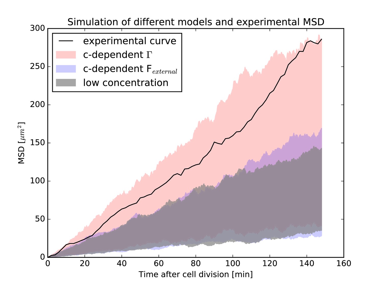
Mean-squared-displacement (MSD) of the first 40 nuclei that could be tracked beginning with cell division in the experiment.

The black curve is the experimental MSD curve as a function of (cell-internal) time after cell division. The shaded areas represent the simulations of different models. In red is the model that assumes the effect of surrounding nuclei is due to a concentration dependence of the stochastic force (i.e. has a concentration-dependent $Γ$ ). In blue is the model that includes the effect of surrounding nuclei via an additional force $F_{external}$ . In gray is the model for low nuclear concentration for comparison. In each case, the same 40 nuclei as the experiment have been simulated, taking their respective environment (i.e. the surrounding nuclear concentration) into account. In each simulation, the MSD curve was calculated as in the experiment. For each model, simulations were repeated 2500 times and the shaded areas represent the range of values covered by the individual resulting MSD curves for each model. The experimental MSD curve only agrees with the model assuming a concentration-dependent stochastic force.

Incubation temperature has direct effects on IKNM

The diffusion model may also address mechanistic questions about IKNM in retinas growing under varying experimental conditions. Zebrafish embryos are often grown at different temperatures to manipulate their growth rate (Kimmel et al., 1995; Reider and Connaughton, 2014), but it has been unclear how the nuclei in the retina behave at these different temperatures. To examine this issue, we grew the embryos at the normal temperature of 28.5 °C overnight and then incubated them at lower temperature (LT) of 25 °C or higher temperature (HT) of 32 °C during imaging. We could directly measure the change in average cell cycle length from experimental data and found that in HT, it is 205.5 min, while in LT, it is a much larger 532.78 min. We were then able to use these values in the model to investigate whether the change in temperature influences the processes that determine the effective diffusion constant of the nuclei. The resulting values for $D_{nonlin}^{*}$ are summarized in Table 1. Based on these values, two-sided t-tests (see Materials and methods) confirmed that there is no significant difference between the D-values obtained from the two normal condition data sets. In contrast, D-values for the LT and HT data sets were significantly different from the normal ones, with $p \leq 0.01$ . These results indicate, that aside from its effect on cell cycle length, incubation temperature is likely to influence IKNM directly by altering the mobility of nuclei, here represented by the effective diffusion constant D.

Discussion

In this work, we have shown that high-density nuclear trajectories can be used to tease apart the possible physical processes behind the apparently stochastic movement of nuclei during interkinetic nuclear migration. First, we acquired these trajectories using long-term imaging and tracking of nuclei with high spatial and temporal resolution within a three-dimensional segment of the zebrafish retina. Analysis of speed and positional distributions of more than a hundred nuclei revealed a large degree of variability in their movements during G1 and S phases. Although this variability had been observed before, previous experiments had only considered sparsely labeled nuclei within an otherwise unlabeled environment (Baye and Link, 2007; Norden et al., 2009; Leung et al., 2011). Thus, our results provide an important account of the variability of IKNM on a whole tissue level. In effect, the variability in IKNM means that nuclear trajectories appear stochastic during the majority of the cell cycle. Previously, it had been suggested that the origins of this apparent stochasticity lay in the transfer of kinetic energy between nuclei in G2 exhibiting rapid apical migration to nuclei in G1 and S phases of the cell cycle, much as a person with an empty beer glass may nudge away other customers to get to the bar (Norden et al., 2009). However, we found no evidence for direct transfer of kinetic energy between nuclei and their immediate neighbors. Recently, Shinoda et al., 2018 have also provided evidence that suggests direct collisions do not contribute to basal IKNM.

Another possibility is that the stochastic trajectories of G1 and S nuclei could be a result of nuclear crowding at the apical surface (Miyata et al., 2014), which, in effect, gives rise to a nuclear concentration gradient from the apical to the basal side of the tissue. This gradient is formed and sustained by nuclear divisions taking place exclusively at the apical surface. While the newly divided daughter nuclei are approximately 0.8 the size of M phase nuclei within the first 10 min after division, they increase in size in the following 10 min to become statistically indistinguishable from M phase nuclei. Thus, the difference in the nuclear density apicobasally is unlikely to be a direct result of variability in nuclear sizes during cell cycle. We confirmed the presence of a nuclear concentration gradient by calculating the nuclear concentration along the apicobasal dimension within the retinal tissue at various time points. Furthermore, to probe the source of the gradient, we treated the zebrafish retina with HU-AC to stop the cell cycle in S phase. While we observed the build-up of the nuclear concentration gradient over time in the control retina, the nuclear distribution flattened when cell division was inhibited with HU-AC treatment. Recent work indicates that only a small fraction of the apical tissue surface is occupied by mitotic cells at any given time (Matejčić et al., 2018). Nonetheless, even this small fraction consistently adds to the number of cells at the apical surface (Figure 5A) contributing to the observed evolving gradient shown in Figure 6.

These phenomenological similarities between IKNM and diffusion suggested a model that includes two key features: firstly, it focuses on the crowding of nuclei at the apical surface of the tissue, here included as the apical boundary condition. Secondly, in the nonlinear extension of the model, it incorporates a maximum possible nuclear concentration. This addition provided a striking overall improvement to the fits to experimental data over periods of many hours. The resulting difference in the obtained D-values between the linear and nonlinear versions of our model can be understood heuristically when closely examining the difference between Equations 1 and 9. The latter introduces the new term $c_{max} / (c_{max} - c)$ which one could think of loosely as corresponding to an effective, concentration dependent diffusion constant $\tilde{D} = D c_{max} / (c_{max} - c)$ . In general, $\tilde{D}$ will vary across the tissue thickness and, since c is nonzero for most of the retinal tissue, $\tilde{D} > D$ . Therefore, averaging across the retinal tissue, $\tilde{D}$ may actually be in very good agreement with the D-value found in the linear model. However, the linear model fails to describe the concentration-dependent nuclear mobility, which is successfully captured in the nonlinear model.

We made further use of the above correspondence between the linear and nonlinear models to obtain a microscopic interpretation of the particular value we obtained for $D_{nonlin}^{*}$ , since both models converge into one another at $c \to 0$ . The value of $D^{*}$ can neither be understood by assuming simple thermal diffusion of the nuclei, nor by simply including effects of membrane-hindered diffusion. Instead, it appears that both hindering and nonequilibrium driving forces have to be included, where nuclear mobility can be slowed-down due to the presence of the membrane and cytosolic composition and sped-up through active transport. Assuming membrane effects and active transport in a Langevin-type model for nuclei at low densities provided an estimate for the strength of the required transport forces, which is consistent with cytoskeletal transport of the nuclei throughout the cell cycle.

We then extended the Langevin-type model for individual nuclei to include the effects of high nuclear packing densities. The resulting models provided a possibility of exploring the properties of individual nuclear trajectories under conditions similar to those found in the experiments. Simulations using different models suggested that the effects of the dense nuclear packing influence the nuclear mobility by locally increasing the strength of the stochastic force. Importantly, the MSD curves obtained in the presence of crowding are essentially linear, even though the underlying dynamics are definitely nonlinear. This illustrates clearly the fact that the linearity of an MSD is not, by itself, particularly probative of the underlying diffusive dynamics.

The underlying processes causing IKNM during the G1 and S phases of the cell cycle in pseudostratified epithelia have been largely elusive. Several partially competing ideas have been put forward, ranging from the active involvement of cytoskeletal transport processes to passive mechanisms of direct energy transfer or movements driven by apical nuclear crowding (Schenk et al., 2009; Tsai et al., 2010; Norden et al., 2009; Kosodo et al., 2011). The fact that inanimate microbeads migrate much like nuclei during IKNM in the mouse cerebral cortex (Kosodo et al., 2011) suggests that active, unidirectional intracellular transport mechanisms are not directly responsible for these stochastic movements. Instead, we show that a passive diffusive process which takes steric interactions between nuclei into account produces an excellent representation of the time evolution of the actual nuclear distribution within the retinal tissue during early development. Consequently, our work builds on earlier models of apical crowding based on in silico simulations of IKNM (Kosodo et al., 2011). However, in contrast to earlier studies, we explicitly account for the dense nuclear packing within the zebrafish retina. Furthermore, we provide an interpretation for the general scale of the diffusion constant (D ∼ 0.1 μm²/min) from microscopic considerations, similar to those used to relate random walks to diffusion (Goldstein, 2018). The results of these microscopic considerations strongly suggest that nuclei are moved by means of cytoskeletal transport throughout the entirety of the cell cycle. However, this transport appears not to be unidirectional but highly stochastic during basal IKNM.

Finally, an extension of the single nuclei equations to high concentrations and the results of stochastic simulations of nuclear trajectories suggest that the stochastic forcing of nuclei itself is concentration-dependent. On a microscopic scale, this can be interpreted, for example, under the assumption that cells can sense the nuclear packing density. If they recruited more molecular motors to areas where nuclei are particularly densely packed, the strength of the stochastic transport forces would be concentration-dependent. Nuclei would thus be transported away from areas of high nuclear packing faster. In addition to these microscopic considerations, our work reveals the importance of simple physical constraints imposed by the overall tissue architecture, which could not be explored in previous studies which tracked sparse nuclei, and thus lacked the means to explore the effect of such three-dimensional arrangements. Hence, we paid special attention to the spherical shape of the retina and the concentration of nuclei in that space. Examining the evolution in distribution of nuclei over time unveils the importance of spatial restriction due to the curvature of the tissue. Additionally, the size of the nuclei in comparison to the tissue leads to the emergence of a maximum nuclear concentration which must be taken into account to model IKNM accurately.

By inhibiting cell cycle progression or changing temperature, we used the model to shed light on properties and mechanisms of the stochastic movements of nuclei during IKNM. From our results and previous studies, we know that cell cycle length is affected by change in incubation temperature (Kimmel et al., 1995; Reider and Connaughton, 2014). However, our results also indicate a significant influence of temperature on the mobility of nuclei and thus the underlying processes controlling their movement. This is reasonable in the light of our microscopic interpretations, which suggested that nuclei move due to cytoskeletal transport through the entire cell cycle in IKNM. The fact that the speed and dynamic properties of both the microtubule and actomyosin systems are temperature dependent may explain the changes in the diffusion constant that we see as a function of temperature (Hartshorne et al., 1972; Hong et al., 2016). In particular, as thermal diffusion is dependent on absolute temperature so the changes in temperature used in these experiments would have little effect on thermal diffusion. Furthermore, disparate observations seem to agree with such an interpretation. For example, a microtubule cage was observed around RPC nuclei (Norden et al., 2009) and myosin was also shown to surround these nuclei (Leung et al., 2011). Disruption of a microtubule motor (dynactin-1) functionality either by mutation (Del Bene et al., 2008) or introduction of a dominant negative allele (Norden et al., 2009) leads to a more basal positioning of nuclei and occasional bursts of basal movement. A conjecture consistent with these observations would be that during G1 and S phases actomyosin based forces push the nucleus basally, as also seen in the mouse telencephalon (Schenk et al., 2009), while microtubule motors push it apically. Finally, in G2 a concentration of myosin at the basal side of the nucleus leads to its rapid apical migration (Leung et al., 2011). However, a much closer examination of molecular mechanisms driving stochastic nuclear movements is required to better understand the connections between these phenomena, as we are far from understanding the nature of all the different forces involved in this process (Kirkland et al., 2020). Furthermore, the diffusion constant reported here reflects all types of nuclear movement during IKNM as it is derived from the changing nuclear concentration profile over time. It is not immediately clear how rapid apical migration contributes to this overall diffusion constant. Nonetheless, despite the large displacement during rapid apical migration at G2, this phase only accounts for about 8% of the cell cycle in RPCs (Leung et al., 2011). Therefore, the good agreement of our calculated diffusion constant with those previously reported in the literature for individual nuclei (Leung et al., 2011) suggests that the proposed model describes tissue-wide IKNM quite well. At the same time, it raises interesting new questions, such as how cells sense such concentrations and the mechanisms that increase the stochastic force on nuclear movement at higher concentrations.

The physiological consequences of nuclear arrangements and IKNM associated with all pseudostratified epithelia are not well understood. Our results provide a quantitative description of the stochastic distribution of the nuclei across the retina. This distribution has been implicated in stochastic cell fate decision making of progenitor cells during differentiation (Clark et al., 2012; Baye and Link, 2007; Hiscock et al., 2018). Our observations would fit with previous suggestions that a signalling gradient, such as Notch, exists across the retina and location-dependent exposure to it is important for downstream decision-making (Murciano et al., 2002; Del Bene et al., 2008; Hiscock et al., 2018; Aggarwal et al., 2016). Thus, our results not only have important implications for understanding the organization of developing vertebrate tissues, but may also provide a starting point for further exploration of the connection between variability in nuclear positions and cell fate decision making in neuroepithelia.

Materials and methods

Animals and transgenic lines

Request a detailed protocol

All animal works were approved by Local Ethical Review Committee of the University of Cambridge and performed in accordance with a Home Office project license PL80/2198. All zebrafish were maintained and bred at 26.5 °C. All embryos were incubated at 28.5 °C before imaging sessions. At 10 hr post-fertilization (hpf), 0.003% phenylthiourea (PTU) (sigma) was added to the medium to stop pigmentation in the eye.

Lightsheet microscopy

Request a detailed protocol

Images of retinal development for the main data set were obtained using lightsheet microscopy. Double transgenic embryos, Tg(bactin2:H2B-GFP::ptf1a:DsRed) were dechorionated at 24 hpf and screened positive for the fluorescent transgenic markers prior to the imaging experiment. The embryo selected for imaging was then embedded in 0.4% low gelling temperature agarose (Type VII, Sigma-Aldrich) prepared in the imaging buffer (0.3x Daniau's solution with 0.2% tricaine and 0.003% PTU [Godinho, 2011]) within an FEP tube with 25 µm thick walls (Zeus), with an eye facing the camera and the illumination light shedding from the ventral side. The tube was held in place by a custom-designed glass capillary (3 mm outer diameter, 20 mm length; Hilgenberg GmbH). The capillary itself was mounted vertically in the imaging specimen chamber filled with the imaging buffer. To ensure normal development, a perfusion system was used to pump warm water into the specimen chamber, maintaining a constant temperature of 28.5 ºC at the location of the specimen.

Time-lapse recording of retinal development was performed using a SiMView light-sheet microscope (Tomer et al., 2012) with one illumination and one detection arm. Lasers were focused by Nikon 10x/0.3 NA water immersion objectives. Images were acquired with Nikon 40x/0.8 NA water immersion objective and Hamamatsu Ocra Flash 4.0 sCMOS camera. GFP was excited with scanned light sheets using a 488 nm laser, and detected through a 525/50 nm band pass detection filter (Semrock). Image stacks were acquired with confocal slit detection (Baumgart and Kubitscheck, 2012) with exposure time of 10 ms per frame, and the sample was moved in 0.812 µm steps along the axial direction. For each time point, two 330 × 330 × 250 µm³ image stacks with a 40 µm horizontal offset were acquired to ensure the coverage of the entire retina. The images were acquired every 2 min from 30 hpf to 72 hpf. The position of the sample was manually adjusted during imaging to compensate for drift. The two image stacks in the same time point were fused together to keep the combined image with the best resolution. An algorithm based on phase correlation was subsequently used to estimate and correct for the sample drift over time. The processing pipeline was implemented with MATLAB (MathWorks).

Two photon microscopy

Request a detailed protocol

Images for the repetition data set and all other conditions were obtained using a TriM Scope II 2-photon microscope (LaVision BioTec). A previously established Tg(H2B-GFP) line, generated by injecting a DNA construct of H2B-GFP driven from the actin promoter (He et al., 2012), was used for all these experiments. Embryos were dechorionated and screened for expression of GFP at 24 hpf. An embryo was then embedded in 0.9% UltraPure low melting point agarose (Invitrogen) prepared in E3 medium containing 0.003% PTU and 0.2% tricaine. The agarose and embryo were placed laterally within a 3D printed half cylinder of transparent ABS plastic, 0.8 mm in diameter, attached to the bottom of a petri dish, such that one eye faced the detection lens of the microscope. The petri dish was then filled with an incubation solution of E3 medium, PTU, and tricaine in the same concentrations as above. For the experiment involving cell cycle arrest, hydroxyurea and aphidicolin (Abcam) were added to the incubation solution right before imaging, to a final concentration of 20 mM and 150 µM, respectively. The imaging chamber was maintained at a temperature of 25 °C, 28.5 °C, or 32 °C, as required, using a precision air heater (The Cube, Life Imaging Services).

Green fluorescence was excited using an Insight DeepSee laser (Spectra-Physics) at 927 nm. The emission of the fluorophore was detected through an Olympus 25x/1.05 NA water immersion objective, and all the signals within the visible spectrum were recorded by a sensitive GaAsP detector. Image stacks with step size of 1 μm were acquired with exposure time of 1.35 ms per line averaged over two scans. The images were recorded every 2 min for 10–15 hrs starting at 26–28 hpf. The same post-processing procedure for data compression and drift correction was used on these raw images as on those from lightsheet imaging.

Obtaining experimental input values for the model

Request a detailed protocol

The radial coordinates $r_{n}$ of nuclei were calculated by subtracting $l_{n}$ from a, wherein $l_{n}$ is the distance from the center of a nucleus n to the apical surface and a is the distance from the center of the lens to the apical surface. We estimated a total uncertainty of $Δ r = \pm 3$ µm for each single distance measurement of $r_{n}$ . This value is a result of uncertainty in detecting the center of the nucleus and in establishing the position of the apical surface.

Because each nuclear position has an error bar $Δ r$ , binning the data leads to an uncertainty in the bin count. In order to calculate this uncertainty, we considered the probability distribution of a nucleus’ position. In the simplest case, this probability is uniform within the width of the positional error bar and zero elsewhere. The probability, $p_{n, bin}$ , of finding a given nucleus n within a given bin, is proportional to the size of the overlap of probability distribution and bin. It follows that the expectation value for the number of nuclei within a bin is given as $E (N_{bin}) = \sum_{n} p_{n, bin}$ . Correspondingly, $Var (N_{bin}) = \sum_{n} p_{n, bin} (1 - p_{n, bin})$ is the variance of the number of nuclei within this bin. Thus, the error bar of the bin count is $σ_{y, bin} = \sqrt{Var (N_{bin})}$ . The nuclear distribution profile $N (r, t)$ is not expected to be uniform or linear, therefore the expectation value $E (N_{bin})$ does not correspond to the number of nuclei at the center of the bin. Since the position of the expectation value is unknown a priori, it is still plotted at the center of the bin with an error bar denoting its positional uncertainty. Here we assume this error bar to be the square-root of the bin size $Δ r_{bin}$ , that is, $σ_{x, bin} = \sqrt{Δ r_{bin}}$ .

In order to obtain the experimental nuclear concentration profile $c (r, t)$ , and its error bars, from the distribution of nuclei $N (r, t)$ , the volume of the retina also has to be taken into account, since $c = N / V$ . The total retinal volume within which nuclei tracking took place was estimated directly from the microscopy images. To this end, we outlined the area of observation in each image slice using the Fiji software and multiplied this area with the distance between successive images. Given the total volume, $V_{total}$ , we proceeded to calculate the volume per bin, which depends on the radii at the inner and outer bin surfaces. In general, the volume of a spherical sector is $V_{sector} = \frac{1}{3} Ω r_{sector}^{3}$ , where $Ω$ denotes the solid angle. Knowing the apical and basal tissue radii, $r = a$ and $r = b$ , one can thus calculate $Ω$ as $Ω = 3 V_{total} / (a^{3} - b^{3})$ . This gives the volume of each bin as $V_{bin} = \frac{1}{3} Ω (r_{bin,outer}^{3} - r_{bin,inner}^{3})$ , where $r_{bin,outer}$ and $r_{bin,inner}$ denote the outer and inner radii of a bin, respectively. Similarly, we calculated the effective surface area S through which the influx of nuclei occurs (see Equation 3) from the solid angle $Ω$ . This surface area is simply given as $S = Ω a^{2}$ .

To retrieve the average cell cycle time $T_{P}$ for each of the data sets, we used two different approaches. In the case of the main data set, sufficient number of nuclear tracks consisting of a whole cell cycle were present. Thus, we directly calculated the average cell cycle duration from these tracks. For the other data sets, we make use of the fact that the number of nuclei follows an exponential growth law depending on $T_{P}$ (see Equation 2). Knowing the initial number of tracked nuclei $N_{0}$ for each data set, we obtained $T_{P}$ from fitting the following equation to the number of nuclei as a function of time in a log-lin plot: $\ln N (t) = \ln N_{0} + t / τ = \ln N_{0} + (\ln 2 / T_{P}) t$ . Then $T_{P}$ was deduced from the slope of this fit.

In order to determine the maximum nuclear concentration $c_{max}$ for the nonlinear model, we first randomly selected 100 nuclei from our dataset of tracked nuclei and measured the size of their longest diameter in both XY and YZ planes. From these measurements, we established that the size of the principal semi-axis of each nucleus is likely to lie in the range of about 3 µm to 5 µm, where the nuclear shape is regarded to be ellipsoidal. This led to the range of possible maximum concentrations $c_{max}$ , although we did not measure the precise nuclear volume. The lower limit for the nuclear volume is set by the volume of a sphere of radius 3 µm, the upper limit by a sphere of radius 5 µm. Taking into account the maximum possible packing density of nuclei, which for aligned ellipsoids is the same as that of spheres (Donev et al., 2004), $π / (3 \sqrt{2}) \approx 0.74$ , we obtained a range of $1.41 \times 10^{- 3} μ m^{- 3} \leq c_{m a x} \leq 6.55 \times 10^{- 3} μ m^{- 3}$ .

Obtaining the initial condition

Request a detailed protocol

We determined the prefactors $h_{i}$ from the experimental nuclear distribution at the start of the experiment, $c_{exp} (ξ, 0)$ . For convenience, we chose to determine first $\tilde{h_{i}} = h_{i} + α_{i} f_{0} / (σ + λ_{i}^{2})$ and then obtained $h_{i}$ by subtracting $α_{i} f_{0} / (σ + λ_{i}^{2})$ from the results. The $\tilde{h_{i}}$ can be calculated from the data, using Equation 6 for $s = 0$ , as

\tilde{h_{i}} = \sum_{m} ξ_{m}^{2} H_{i} (ξ_{m}) c_{exp} (ξ_{m}, 0) Δ ξ_{m} - \frac{f_{0}}{1 - ρ} \int_{ρ}^{1} ξ^{2} H_{i} (ξ) (\frac{1}{2} ξ^{2} - ρ ξ + g_{0}) 𝑑 ξ,

where m denotes the m-th binned data point, $ξ_{m}$ its position and $Δ ξ_{m}$ the width of bin m. As in Equation 6, the index i denotes the i-th eigenfunction or -mode.

The concentration profile in the nonlinear model

Request a detailed protocol

The non-linear concentration profile was determined numerically from the same initial condition as used for the linear model, Equation 6, at $s = 0$ with $\tilde{h_{i}}$ as in Equation 17. Time evolution of the initial condition, according to Equation 9, was performed using the pdepe solver in MATLAB.

Fitting the model

Request a detailed protocol

The range of sizes of the nuclear principal semi-axes was used to determine the range of data to be included in our fits. Any data closer than 3 µm to 5 µm from the apical or basal tissue surfaces was not taken into account for fitting because the center of a nucleus cannot be any closer to a surface than the nuclear radius. Thus, all data collection very close to the apical or basal tissue surfaces must have been due to the above-mentioned measurement uncertainties $Δ r$ .

In principle, the full solution for $c (ξ, s)$ is composed of infinitely many modes. However, in practice, we truncated this series and only included the first eight modes in our fits. This is due to the fact that we have a finite set of data points, so adding too many modes could lead to over-fitting. Fits with a wide range of numbers of modes were found to result in the same optimal D-values.

For fitting, we first rescaled the data in accordance with the non-dimensionalization of the theoretical variables r and t (see Equation 5). Thus we obtain $c_{exp} (ξ, s)$ from $c_{exp} (r, t)$ . Then both models were fitted to the experimental data using a minimal- $χ^{2}$ approach. The goodness of fit parameter $χ^{2} = \sum_{m} {(c_{exp} (ξ, s) - c (ξ, s))}^{2} / σ_{m}^{2}$ , where $\sum_{m}$ denotes the summation over all bins m. Since binning resulted in uncertainties $σ_{y, bin}$ and $σ_{x, bin}$ in the y- and x-directions, both had to be taken into account when calculating $σ_{m}$ and $χ^{2}$ . The combined contribution of x- and y- uncertainties is: $σ_{m}^{2} = σ_{y, m}^{2} + σ_{y, indirect, m}^{2}$ with $σ_{y, indirect, m} = {σ_{x, m} (d c (ξ, s) / d ξ) |}_{ξ = ξ_{m}}$ (Bevington and Robinson, 2003). In our fits, the value $χ^{2}$ was calculated for a large range of possible diffusion constants D, from $D = 0.01$ µm²/min to $D = 10$ µm²/min. By finding the value of D for which $χ^{2}$ became minimal for a given data set and time point, we established our optimal fit.

The minimal- $χ^{2}$ approach furthermore enabled us to determine the optimal binning width $Δ r_{bin}$ or $Δ ξ_{bin}$ and width of data exclusion for the fits. In order to do so, fits of the normal data set were performed for different data binning widths and exclusion sizes of 3 µm to 5 µm. For each of these fits the $χ^{2}$ -value and the number of degrees of freedom ν, that is, the number of data points minus the number of free fit parameters (here number of data points minus 1), were registered. From $χ^{2}$ and ν, we calculated the reduced $χ^{2}$ value, $χ_{ν}^{2} = χ^{2} / ν$ (Bevington and Robinson, 2003). Using ν and $χ_{ν}^{2}$ , the probability $P_{χ} (χ^{2}; ν)$ of exceeding $χ^{2}$ for a given fit can be estimated, which should be approximately 0.5 (Bevington and Robinson, 2003). Therefore, we found our optimal data binning width of 3 µm to 4 µm as the width that resulted in a $P_{χ} (χ^{2}; ν)$ as close to 0.5 as possible for all the different time points when fitting the nonlinear model. The exact choice of exclusion width was found not to influence the fitting result for the nonlinear model.

In addition to finding the optimal D-value for individual time points, we also modified the minimal- $χ^{2}$ routine to find the value of D that fits a whole data set (i.e. all time points simultaneously) in the best possible way. In order to do so, we summed the $χ^{2}$ -values obtained for each D over all time points, in this way producing a $\sum_{t} χ^{2} (D)$ -curve. The minimum of this curve indicates $D^{*}$ for the whole time series. Furthermore, dividing $\sum_{t} χ^{2} (D)$ by the number of time points included in the optimization yields an average $χ^{2}$ - and reduced $χ^{2}$ -value corresponding to this $D^{*}$ . In addition, the width of this time averaged curve at $χ^{2} = χ_{min}^{2} + 1$ indicates the standard deviation of the optimal D-value, $σ_{D}$ . By approximating the minimum with a quadratic curve, we obtain an estimate for this standard deviation as $σ_{D} = Δ_{D} \sqrt{2 (χ_{D^{*} - Δ_{D}}^{2} - 2 χ_{D^{*}}^{2} + χ_{D^{*} + Δ_{D}}^{2})}$ (Bevington and Robinson, 2003) where $Δ_{D}$ is the step size between individual fitted D-values, here $Δ_{D} = 0.01$ µm²/min. Lastly, based on the average reduced $χ^{2}$ -values, we also compared several $c_{max}$ -values for each data set to find the fit with probability $P_{χ} (χ^{2}; ν)$ the closest to 0.5 in each case.

All fits were performed using custom MATLAB routines. Horizontal error bars were plotted using the function herrorbar (van der Geest, 2006).

Nuclear radius for interpretation of D

Request a detailed protocol

The average nuclear radius used to calculate the friction coefficient and thermal diffusion coefficient of IKNM nuclei was the radius corresponding to the maximum concentration $c_{max}$ obtained from the fitting procedure.

Experimental nuclear birth times and mean-squared-displacement curve

Request a detailed protocol

Among all the nuclei tracked in the experiments, we selected those nuclei where tracking data was available beginning right from cell division and also over a sufficiently long period of time to cover a substantial part of the cell cycle (at least 75 time steps, i.e. 150 min). For these nuclei, we extracted their respective birth times within the experiment from the full tracks and sorted the nuclei accordingly. The first 40 nuclei were chosen for further analysis, as these were nuclei with a minimum of 150 min of tracking data completely within the first 200 min of experiments, corresponding to the time frame used for D-optimization in the non-linear diffusion model. The exact distribution of their birth times was stored for use in the individual nuclei simulations.

Further, the nuclear tracks of the chosen 40 nuclei were transformed from being a function of experimental time to being a function of cell cycle time by simply subtracting a nucleus individual birth time from the experimental time for each step of its tracking data. Then the experimental mean squared displacement curve was calculated from the so obtained cell-cycle-dependent tracks.

Calculation of the shapes of retinal cell shapes

Request a detailed protocol

Here, we give more information on the numerical calculation of cell shapes. Further details can be found elsewhere (Herrmann, 2020). Minimization of the elastic energy (Equation 12) leads to the equilibrium condition on the shape, expressed in terms of the mean curvature $ℋ$ and the Gaussian curvature $𝒦$ (Zhong-can and Helfrich, 1989),

- γ ℋ + 2 κ (ℋ^{3} - 𝒦 ℋ) + κ Δ ℋ = 0,

where, for an axisymmetric shape $δ (z)$ ,

𝒦 = - \frac{δ_{z z}}{δ {(1 + δ_{z}^{2})}^{2}}

and $Δ$ is the Laplacian operator,

\nabla^{2} = \frac{1}{δ \sqrt{1 + δ_{z}^{2}}} \frac{\partial}{\partial z} (\frac{δ}{\sqrt{1 + δ_{z}^{2}}} \frac{\partial}{\partial z}) .

The resulting shape equation is fourth order in z-derivatives and thus requires four boundary conditions. Given the symmetry of the system, we solve for the shape in the left half of the domain $z = (0, L / 2)$ and impose $δ (0) = δ_{a}$ and $δ_{z} (0) = 0$ at the apical surface. Imposing boundary conditions like $δ (L / 2) = R$ and $δ_{z} (L / 2) = 0$ at the top of the nucleus usually leads to solutions that are incompatible with the presence of the nucleus (the resulting membrane shapes would cut through the nucleus). Therefore, we further divide the domain $z = (0, L / 2)$ into a region away from the nucleus and a region where the membrane is in close contact with it. In the latter region, we assume the membrane to be bent into a spherical arc around the nucleus, leaving a small equilibrium gap as estimated by Daniels, 2019. The contact point $z_{contact}$ between the two regions is adjusted until the membrane radius and its derivative are continuous through the contact point. The membrane shape away from the nucleus is then found using the MATLAB bvp5c solver. As can be seen from energy minimization using (Equation 12), the solution in each case turns out to be the one for which $z_{contact}$ has been chosen such that the resulting $ℋ$ in $z \in [0, z_{contact}]$ is equal to $ℋ_{c i r c l e} = - 1 / R_{t u b e}$ for $z \to z_{contact}$ , where $R_{t u b e}$ is the radius of the membrane arc around the nucleus.

Simulations of individual nuclear trajectories

Request a detailed protocol

Simulations of nuclear trajectories for each of the three Langevin-type models were performed using a custom Python 3 routine. Time discretization of the stochastic differential equations was achieved via the Euler-Maruyama method. Simulations were performed using 0.2 min time steps and were checked against those with smaller time steps to ensure that this choice was sufficiently small.

In each run of a simulation, 40 nuclei were simulated and their birth times within the simulation were chosen to be the same birth times as those obtained from the nuclei within the experiments. Each nucleus was simulated for a total of 150 min, corresponding to the chosen experimental data. The value for the diffusion constant in these simulations was set to be the previously obtained value $D_{nonlin}^{*}$ . For simulations with nuclear concentration-dependent Langevin equations, $c_{max}$ and the average nuclear concentration field $c (r, t)$ were similarly extracted from the results of the previous fits using the non-linear diffusion equation. Herein, $c (r, t)$ was provided for each time step of the simulation. As $c (r, t)$ can only be provided for discrete spatial coordinates r but the Langevin-type simulations were continuous in the spatial coordinate r, c was averaged over the values at the two closest spatial points whenever a nucleus' position did not exactly coincide with a point where the value for c was provided.

The resulting simulated nuclear trajectories were treated in the same way as the experimentally obtained ones. That is, the nuclei's birth times were subtracted from the trajectories to obtain cell cycle dependent tracks. Then, the mean squared displacement curve was calculated from the resulting set.

For each model, the same simulation was repeated 2500 times to obtain the range of distributions of the resulting mean squared displacement curves. For each cell cycle time step, the minimum and maximum of the mean squared displacement values out of all 2500 repetitions were calculated to obtain the areas depicted in Figure 8.

t-tests

Request a detailed protocol

To compare results between data sets, the values $D^{*}$ and corresponding $σ_{D}$ from the overall fits were considered. It should be noted that these values were not obtained by averaging several data sets of the same experimental condition but instead each value results from one data set only. However, the sample size for each data set was set to 100 because 100 time points were taken into account for each overall optimization. These time points might not be completely uncorrelated, limiting the predictive power of the t-test. Two sided tests, specifically unequal variances t-test, also known as Welch’s t-test, (Precht and Kraft, 2015), were performed in order to determine whether samples differ significantly from each other.

Description of Matlab files

Request a detailed protocol

Source code files 1, 2, 3, 4, 5, 6 are Matlab files containing the tracking data, as follows.

Appendix 1

Full solution of the linear diffusion equation

After rescaling space and time as in Equation 5 and introducing $ρ = b / a < 1$ , Equation 1 and the boundary conditions Equation 3 and Equation 4 read

\begin{array}{ll} \frac{\partial c (ξ, s)}{\partial s} = \frac{1}{ξ^{2}} \frac{\partial}{\partial ξ} (ξ^{2} \frac{\partial c (ξ, s)}{\partial ξ}), \\ {\frac{\partial c (ξ, s)}{\partial ξ} |}_{ξ = 1} = f_{0} e^{σ s} = f (s) and {\frac{\partial c (ξ, s)}{\partial ξ} |}_{ξ = ρ} = 0, \end{array}

where we have defined $f_{0} = a N_{0} / D S τ$ and $σ = a^{2} / D τ$ . We transform this homogeneous differential equation with inhomogeneous boundary conditions into the problem of solving an inhomogeneous differential equation with homogeneous boundary conditions by writing $c (ξ, s)$ as a sum of two contributions,

c (ξ, s) = ϕ (ξ, s) + ψ (ξ, s),

where we require $ϕ (ξ, s)$ to satisfy the inhomogeneous boundary conditions

{\frac{\partial ϕ (ξ, s)}{\partial ξ} |}_{ξ = 1} = f_{0} e^{σ s} and {\frac{\partial ϕ (ξ, s)}{\partial ξ} |}_{ξ = ρ} = 0.

These conditions are satisfied if $ϕ (ξ, s)$ has the form

ϕ (ξ, s) = \frac{1}{1 - ρ} (\frac{1}{2} ξ^{2} - ρ ξ + g_{0}) f_{0} e^{σ s} .

where $g_{0}$ is a constant of integration to be determined later. The remaining problem to solve for $ψ (ξ, s)$ is

\frac{\partial ψ (ξ, s)}{\partial s} = \frac{1}{ξ^{2}} \frac{\partial}{\partial ξ} (ξ^{2} \frac{\partial ψ (ξ, s)}{\partial ξ}) + \frac{f_{0} e^{σ s}}{1 - ρ} (3 - \frac{2 ρ}{ξ} - σ (\frac{1}{2} ξ^{2} - ρ ξ + g_{0})),

with homogeneous boundary conditions

{\frac{\partial ψ (ξ, s)}{\partial ξ} |}_{ξ = 1} = 0 and {\frac{\partial ψ (ξ, s)}{\partial ξ} |}_{ξ = ρ} = 0.

We can further write $ψ (ξ, s)$ as the sum of two contributions,

ψ (ξ, s) = ψ_{h} (ξ, s) + ψ_{p} (ξ, s),

where $ψ_{h}$ is the general solution of the homogeneous problem

\begin{array}{ll} \frac{\partial ψ_{h} (ξ, s)}{\partial s} = \frac{1}{ξ^{2}} \frac{\partial}{\partial ξ} (ξ^{2} \frac{\partial ψ_{h} (ξ, s)}{\partial ξ}), \\ {\frac{\partial ψ_{h} (ξ, s)}{\partial ξ} |}_{ξ = 1} = 0 and {\frac{\partial ψ_{h} (ξ, s)}{\partial ξ} |}_{ξ = ρ} = 0, \end{array}

and $ψ_{p}$ is a particular solution of the full inhomogeneous problem Equation 26. The full solution of the homogeneous problem is given as a series of linearly independent eigenfunctions, each of the form

e^{- λ^{2} s} W (ξ) = e^{- λ^{2} s} (A \frac{\sin λ ξ}{ξ} + B \frac{\cos λ ξ}{ξ}),

where the eigenvalues λ can be found from simultaneous solution of the boundary conditions,

\begin{array}{ll} A (λ \cos λ - \sin λ) - B (λ \sin λ + \cos λ) = 0 \\ A (\frac{λ \cos λ ρ}{ρ} - \frac{\sin λ ρ}{ρ^{2}}) - B (\frac{λ \sin λ ρ}{ρ} + \frac{\cos λ ρ}{ρ^{2}}) = 0, \end{array}

which yields the transcendental relation

\tan λ (1 - ρ) = \frac{λ (1 - ρ)}{λ^{2} ρ + 1},

for which each eigenvalue $λ_{i}$ is a solution corresponding to one of the linearly independent eigenfunctions (only $λ_{i} > 0$ need to be taken into account). We can further deduce from the Equation 30 that $B_{i} = β_{i} A_{i}$ , where

β_{i} = \frac{λ_{i} \cos λ_{i} - \sin λ_{i}}{λ_{i} \sin λ_{i} + \cos λ_{i}},

and we normalize the obtained expression for $W_{i} (ξ)$ from Equation 29

H_{i} (ξ) = \frac{1}{Y_{i}} (\frac{\sin λ_{i} ξ}{ξ} + β_{i} \frac{\cos λ_{i} ξ}{ξ}),

with

Y_{i}^{2} = \frac{1}{2} (1 - ρ) (1 + β_{i}^{2}) - \frac{1}{4 λ_{i}} (\sin 2 λ_{i} - \sin 2 λ_{i} ρ) (1 - β_{i}^{2}) + \frac{β_{i}}{λ_{i}} (\sin^{2} λ_{i} - \sin^{2} λ_{i} ρ) .

Thus, the homogeneous solution $ψ_{h}$ is

ψ_{h} = \sum_{i = 1}^{\infty} h_{i} H_{i} (ξ) e^{- λ_{i}^{2} s},

with prefactors $h_{i}$ to be determined from the initial condition.

In order to find a particular solution of the inhomogeneous problem, we first rewrite Equation 26 as

\frac{\partial ψ (ξ, s)}{\partial s} - \frac{1}{ξ^{2}} \frac{\partial}{\partial ξ} (ξ^{2} \frac{\partial ψ (ξ, s)}{\partial ξ}) = ℛ (ξ, s) .

Now, we express $ℛ (ξ, s)$ , as well as the unknown inhomogeneous solution $ψ_{p} (ξ, s)$ in terms of the normalized eigenfunctions $H (ξ, s)$ of the homogeneous problem,

ℛ (ξ, s) = \sum_{i = 1}^{\infty} R_{i} (s) H_{i} (ξ),

and

ψ_{p} (ξ, s) = \sum_{i = 1}^{\infty} C_{i} (s) H_{i} (ξ) .

Substituting these forms into Equation 36, and noting that each term in the series must vanish separately we obtain

\frac{\partial C_{i} (s)}{\partial s} + λ_{i}^{2} C_{i} (s) - R_{i} (s) = 0 .

From the form of $ℛ (ξ, s)$ it follows that $R_{i} (s) = α_{i} f_{0} e^{σ s}$ with some purely numerical prefactors $α_{i}$ , so we expect $C_{i} (s) \propto p_{i} e^{σ s}$ and find

p_{i} = \frac{α_{i} f_{0}}{σ + λ_{i}^{2}} .

Finally, we determine the $α_{i}$ by reconsidering Equation 37. We multiply both sides by $ξ^{2} H_{j} (ξ)$ , where $H_{j} (ξ)$ is one specific but arbitrary eigenfunction of the homogeneous problem, and then integrate over the whole volume V. By the orthogonormality of these eigenfunctions, we obtain

α_{j} = \int \frac{1}{1 - ρ} (3 - \frac{2 ρ}{ξ} - σ (\frac{1}{2} ξ^{2} - ρ ξ + g_{0})) ξ^{2} H_{j} (ξ) 𝑑 ξ,

and all the $α_{i}$ can be calculated explicitely. Thus, the full solution of the linear problem is

c (ξ, s) = \sum_{i = 1}^{\infty} (h_{i} e^{- λ_{i}^{2} s} + \frac{α_{i} f_{0}}{σ + λ_{i}^{2}} e^{σ s}) H_{i} (ξ) + \frac{1}{1 - ρ} (\frac{1}{2} ξ^{2} - ρ ξ + g_{0}) f_{0} e^{σ s} .

The constant $g_{0}$ can now be calculated from the requirement that $\int c (ξ, s = 0) d V = N_{0}$ . Here, we make use of the fact that $\int H_{i} (ξ) ξ^{2} 𝑑 ξ = 0$ if $λ_{i}$ satisfies Equation 31, thus

g_{0} = \frac{(1 - ρ) / σ - \frac{1}{10} + \frac{1}{4} ρ + \frac{1}{10} ρ^{5} - \frac{1}{4} ρ^{5}}{\frac{1}{3} (1 - ρ^{3})} .

Data availability

All data generated or analysed during this study are included in the manuscript and supporting files.

References

(2016) Concentration sensing by the moving nucleus in cell fate determination: a computational analysis
PLOS One 11:e0149213.
https://doi.org/10.1371/journal.pone.0149213
- PubMed
- Google Scholar
1. Amat F
2. Lemon W
3. Mossing DP
4. McDole K
5. Wan Y
6. Branson K
7. Myers EW
8. Keller PJ
(2014) Fast, accurate reconstruction of cell lineages from large-scale fluorescence microscopy data
Nature Methods 11:951–958.
https://doi.org/10.1038/nmeth.3036
- PubMed
- Google Scholar
1. Amat F
2. Höckendorf B
3. Wan Y
4. Lemon WC
5. McDole K
6. Keller PJ
(2015) Efficient processing and analysis of large-scale light-sheet microscopy data
Nature Protocols 10:1679–1696.
https://doi.org/10.1038/nprot.2015.111
- PubMed
- Google Scholar
1. Avanesov A
2. Malicki J
(2010) Analysis of the retina in the zebrafish model
Methods in Cell Biology 100:153–204.
https://doi.org/10.1016/B978-0-12-384892-5.00006-2
- PubMed
- Google Scholar
1. Bar-Ziv R
2. Moses E
(1994) Instability and "pearling" states produced in tubular membranes by competition of curvature and tension
Physical Review Letters 73:1392–1395.
https://doi.org/10.1103/PhysRevLett.73.1392
- PubMed
- Google Scholar
1. Baranovskiy AG
2. Babayeva ND
3. Suwa Y
4. Gu J
5. Pavlov YI
6. Tahirov TH
(2014) Structural basis for inhibition of DNA replication by aphidicolin
Nucleic Acids Research 42:14013–14021.
https://doi.org/10.1093/nar/gku1209
- PubMed
- Google Scholar
1. Barrasso AP
2. Wang S
3. Tong X
4. Christiansen AE
5. Larina IV
6. Poché RA
(2018) Live imaging of developing mouse retinal slices
Neural Development 13:23.
https://doi.org/10.1186/s13064-018-0120-y
- PubMed
- Google Scholar
1. Baumgart E
2. Kubitscheck U
(2012) Scanned light sheet microscopy with confocal slit detection
Optics Express 20:21805–21814.
https://doi.org/10.1364/OE.20.021805
- PubMed
- Google Scholar
1. Baye LM
2. Link BA
(2007) Interkinetic nuclear migration and the selection of neurogenic cell divisions during vertebrate retinogenesis
Journal of Neuroscience 27:10143–10152.
https://doi.org/10.1523/JNEUROSCI.2754-07.2007
- PubMed
- Google Scholar
Book
1. Bevington PR
2. Robinson DK
(2003) Data Reduction and Error Analysis for the Physical Sciences (3rd edition)
McGraw-Hill.
https://doi.org/10.1063/1.4823194
- Google Scholar
(2001) Onset and time course of apoptosis in the developing zebrafish retina
Cell and Tissue Research 306:199–207.
https://doi.org/10.1007/s004410100447
- PubMed
- Google Scholar
1. Clark BS
2. Cui S
3. Miesfeld JB
4. Klezovitch O
5. Vasioukhin V
6. Link BA
(2012) Loss of Llgl1 in retinal neuroepithelia reveals links between apical domain size, notch activity and neurogenesis
Development 139:1599–1610.
https://doi.org/10.1242/dev.078097
- PubMed
- Google Scholar
1. Daniels DR
(2019) Transport of solid bodies along tubular membrane tethers
PLOS ONE 14:e0210259.
https://doi.org/10.1371/journal.pone.0210259
- PubMed
- Google Scholar
1. Del Bene F
2. Wehman AM
3. Link BA
4. Baier H
(2008) Regulation of neurogenesis by interkinetic nuclear migration through an apical-basal notch gradient
Cell 134:1055–1065.
https://doi.org/10.1016/j.cell.2008.07.017
- PubMed
- Google Scholar
1. Del Bene F
(2011) Interkinetic nuclear migration: cell cycle on the move
The EMBO Journal 30:1676–1677.
https://doi.org/10.1038/emboj.2011.114
- PubMed
- Google Scholar
(2004) Unusually dense crystal packings of ellipsoids
Physical Review Letters 92:255506.
https://doi.org/10.1103/PhysRevLett.92.255506
- PubMed
- Google Scholar
1. Einstein A
(1905) Über die Von der molekularkinetischen theorie der wärme geforderte bewegung von in ruhenden flüssigkeiten suspendierten teilchen
Annalen Der Physik 322:549–560.
https://doi.org/10.1002/andp.19053220806
- Google Scholar
(2007) Direct measurement of force generation by actin filament polymerization using an optical trap
PNAS 104:2181–2186.
https://doi.org/10.1073/pnas.0607052104
- PubMed
- Google Scholar
1. Godinho L
(2011) Imaging zebrafish development
Cold Spring Harbor Protocols 2011:879–883.
https://doi.org/10.1101/pdb.prot5647
- PubMed
- Google Scholar
(1996)
Front propagation in the pearling instability of tubular vesicles

Journal de Physique II 6:767–796.
- Google Scholar
1. Goldstein RE
(2018) Are theoretical results 'Results'?
eLife 7:e40018.
https://doi.org/10.7554/eLife.40018
- PubMed
- Google Scholar
(1972) The effect of temperature on actomyosin
Biochimica Et Biophysica Acta (BBA) - Bioenergetics 267:190–202.
https://doi.org/10.1016/0005-2728(72)90150-8
- Google Scholar
1. He J
2. Zhang G
3. Almeida AD
4. Cayouette M
5. Simons BD
6. Harris WA
(2012) How variable clones build an invariant retina
Neuron 75:786–798.
https://doi.org/10.1016/j.neuron.2012.06.033
- PubMed
- Google Scholar
1. Helfrich W
(1973) Elastic properties of lipid bilayers: theory and possible experiments
Zeitschrift Für Naturforschung C 28:693–703.
https://doi.org/10.1515/znc-1973-11-1209
- PubMed
- Google Scholar
1. Helfrich W
(1978) Steric interaction of fluid membranes in multilayer systems
Zeitschrift Für Naturforschung A 33:305–315.
https://doi.org/10.1515/zna-1978-0308
- Google Scholar
Thesis
1. Herrmann A
(2020)
Nuclei on the move - Physical Aspects of Interkinetic Nuclear Migration. PhD thesis

University of Cambridge.
- Google Scholar
(2018) Feedback between tissue packing and neurogenesis in the zebrafish neural tube
Development 145:dev157040.
https://doi.org/10.1242/dev.157040
- PubMed
- Google Scholar
1. Hong W
2. Takshak A
3. Osunbayo O
4. Kunwar A
5. Vershinin M
(2016) The effect of temperature on Microtubule-Based transport by cytoplasmic dynein and Kinesin-1 motors
Biophysical Journal 111:1287–1294.
https://doi.org/10.1016/j.bpj.2016.08.006
- PubMed
- Google Scholar
Book
1. Huang K
(1987)
Statistical Mechanics (2nd edition)

John Wiley & Sons.
- Google Scholar
(2016) Independent modes of ganglion cell translocation ensure correct lamination of the zebrafish retina
Journal of Cell Biology 215:259–275.
https://doi.org/10.1083/jcb.201604095
- PubMed
- Google Scholar
(1995) Stages of embryonic development of the zebrafish
Developmental Dynamics 203:253–310.
https://doi.org/10.1002/aja.1002030302
- PubMed
- Google Scholar
1. Kirkland NJ
2. Yuen AC
3. Tozluoglu M
4. Hui N
5. Paluch EK
6. Mao Y
(2020) Tissue mechanics regulate mitotic nuclear dynamics during epithelial development
Current Biology 30:2419–2432.
https://doi.org/10.1016/j.cub.2020.04.041
- PubMed
- Google Scholar
1. Kosodo Y
2. Suetsugu T
3. Suda M
4. Mimori-Kiyosue Y
5. Toida K
6. Baba SA
7. Kimura A
8. Matsuzaki F
(2011) Regulation of interkinetic nuclear migration by cell cycle-coupled active and passive mechanisms in the developing brain
The EMBO Journal 30:1690–1704.
https://doi.org/10.1038/emboj.2011.81
- PubMed
- Google Scholar
1. Lemons DS
2. Gythiel A
(1997) Paul Langevin’s 1908 paper “On the Theory of Brownian Motion” [“Sur la théorie du mouvement brownien,” C. R. Acad. Sci. (Paris) 146, 530–533 (1908)]
American Journal of Physics 65:1079–1081.
https://doi.org/10.1119/1.18725
- Google Scholar
(2009) Dynamics of enhanced tracer diffusion in suspensions of swimming eukaryotic microorganisms
Physical Review Letters 103:198103.
https://doi.org/10.1103/PhysRevLett.103.198103
- PubMed
- Google Scholar
1. Leung L
2. Klopper AV
3. Grill SW
4. Harris WA
5. Norden C
(2011) Apical migration of nuclei during G2 is a prerequisite for all nuclear motion in zebrafish neuroepithelia
Development 138:5003–5013.
https://doi.org/10.1242/dev.071522
- PubMed
- Google Scholar
(2018) A non-cell-autonomous actin redistribution enables isotropic retinal growth
PLOS Biology 16:e2006018.
https://doi.org/10.1371/journal.pbio.2006018
- PubMed
- Google Scholar
(2014) Interkinetic nuclear migration generates and opposes ventricular-zone crowding: insight into tissue mechanics
Frontiers in Cellular Neuroscience 8:473.
https://doi.org/10.3389/fncel.2014.00473
- PubMed
- Google Scholar
(2002) Interkinetic nuclear movement may provide spatial clues to the regulation of neurogenesis
Molecular and Cellular Neuroscience 21:285–300.
https://doi.org/10.1006/mcne.2002.1174
- PubMed
- Google Scholar
(1995) Dynamical theory of the pearling instability in cylindrical vesicles
Physical Review Letters 74:3384–3387.
https://doi.org/10.1103/PhysRevLett.74.3384
- PubMed
- Google Scholar
1. Norden C
2. Young S
3. Link BA
4. Harris WA
(2009) Actomyosin is the main driver of interkinetic nuclear migration in the retina
Cell 138:1195–1208.
https://doi.org/10.1016/j.cell.2009.06.032
- PubMed
- Google Scholar
1. Norden C
(2017) Pseudostratified epithelia - cell biology, diversity and roles in organ formation at a glance
Journal of Cell Science 130:1859–1863.
https://doi.org/10.1242/jcs.192997
- PubMed
- Google Scholar
1. Okamoto M
2. Namba T
3. Shinoda T
4. Kondo T
5. Watanabe T
6. Inoue Y
7. Takeuchi K
8. Enomoto Y
9. Ota K
10. Oda K
11. Wada Y
12. Sagou K
13. Saito K
14. Sakakibara A
15. Kawaguchi A
16. Nakajima K
17. Adachi T
18. Fujimori T
19. Ueda M
20. Hayashi S
21. Kaibuchi K
22. Miyata T
(2013) TAG-1-assisted progenitor elongation streamlines nuclear migration to optimize subapical crowding
Nature Neuroscience 16:1556–1566.
https://doi.org/10.1038/nn.3525
- PubMed
- Google Scholar
(1993) Cellular motions and thermal fluctuations: the brownian ratchet
Biophysical Journal 65:316–324.
https://doi.org/10.1016/S0006-3495(93)81035-X
- PubMed
- Google Scholar
Book
1. Precht M
2. Kraft R
(2015) Bio-Statistik 2 (5th edition)
De Gruyter.
https://doi.org/10.1002/bimj.200610281
- Google Scholar
1. Reider M
2. Connaughton VP
(2014) Effects of low-dose embryonic thyroid disruption and rearing temperature on the development of the eye and retina in zebrafish
Birth Defects Research Part B: Developmental and Reproductive Toxicology 101:347–354.
https://doi.org/10.1002/bdrb.21118
- PubMed
- Google Scholar
Book
1. Reif F
(1965)
Fundamentals of Statistical and Thermal Physics (1st edition)

McGraw-Hill.
- Google Scholar
1. Sauer FC
(1935) Mitosis in the neural tube
The Journal of Comparative Neurology 62:377–405.
https://doi.org/10.1002/cne.900620207
- Google Scholar
(2009) Myosin II is required for interkinetic nuclear migration of neural progenitors
PNAS 106:16487–16492.
https://doi.org/10.1073/pnas.0908928106
- PubMed
- Google Scholar
1. Schindelin J
2. Arganda-Carreras I
3. Frise E
4. Kaynig V
5. Longair M
6. Pietzsch T
7. Preibisch S
8. Rueden C
9. Saalfeld S
10. Schmid B
11. Tinevez JY
12. White DJ
13. Hartenstein V
14. Eliceiri K
15. Tomancak P
16. Cardona A
(2012) Fiji: an open-source platform for biological-image analysis
Nature Methods 9:676–682.
https://doi.org/10.1038/nmeth.2019
- PubMed
- Google Scholar
1. Shinoda T
2. Nagasaka A
3. Inoue Y
4. Higuchi R
5. Minami Y
6. Kato K
7. Suzuki M
8. Kondo T
9. Kawaue T
10. Saito K
11. Ueno N
12. Fukazawa Y
13. Nagayama M
14. Miura T
15. Adachi T
16. Miyata T
(2018) Elasticity-based boosting of neuroepithelial nucleokinesis via indirect energy transfer from mother to daughter
PLOS Biology 16:e2004426.
https://doi.org/10.1371/journal.pbio.2004426
- PubMed
- Google Scholar
(1959) Cell proliferation and migration in the primitive ependymal zone: an autoradiographic study of histogenesis in the nervous system
Experimental Neurology 1:322–333.
https://doi.org/10.1016/0014-4886(59)90024-X
- PubMed
- Google Scholar
1. Singh A
2. Xu Y-J
(2016) The cell killing mechanisms of hydroxyurea
Genes 7:99.
https://doi.org/10.3390/genes7110099
- PubMed
- Google Scholar
1. Spear PC
2. Erickson CA
(2012) Interkinetic nuclear migration: a mysterious process in search of a function
Development, Growth & Differentiation 54:306–316.
https://doi.org/10.1111/j.1440-169X.2012.01342.x
- PubMed
- Google Scholar
1. Stelzer EH
(2015) Light-sheet fluorescence microscopy for quantitative biology
Nature Methods 12:23–26.
https://doi.org/10.1038/nmeth.3219
- PubMed
- Google Scholar
(2009) Illuminating cell-cycle progression in the developing zebrafish embryo
PNAS 106:20812–20817.
https://doi.org/10.1073/pnas.0906464106
- PubMed
- Google Scholar
1. Svoboda K
2. Yasuda R
(2006) Principles of two-photon excitation microscopy and its applications to neuroscience
Neuron 50:823–839.
https://doi.org/10.1016/j.neuron.2006.05.019
- PubMed
- Google Scholar
1. Tomer R
2. Khairy K
3. Amat F
4. Keller PJ
(2012) Quantitative high-speed imaging of entire developing embryos with simultaneous multiview light-sheet microscopy
Nature Methods 9:755–763.
https://doi.org/10.1038/nmeth.2062
- PubMed
- Google Scholar
(2007) Dual subcellular roles for LIS1 and dynein in radial neuronal migration in live brain tissue
Nature Neuroscience 10:970–979.
https://doi.org/10.1038/nn1934
- PubMed
- Google Scholar
1. Tsai JW
2. Lian WN
3. Kemal S
4. Kriegstein AR
5. Vallee RB
(2010) Kinesin 3 and cytoplasmic dynein mediate interkinetic nuclear migration in neural stem cells
Nature Neuroscience 13:1463–1471.
https://doi.org/10.1038/nn.2665
- PubMed
- Google Scholar
Website
1. van der Geest J
(2006) Herrorbar
Accessed December 14, 2017.

https://uk.mathworks.com/matlabcentral/fileexchange/3963-herrorbar
1. Wang B
2. Anthony SM
3. Bae SC
4. Granick S
(2009) Anomalous yet brownian
PNAS 106:15160–15164.
https://doi.org/10.1073/pnas.0903554106
- PubMed
- Google Scholar
1. Wolff C
2. Tinevez JY
3. Pietzsch T
4. Stamataki E
5. Harich B
6. Guignard L
7. Preibisch S
8. Shorte S
9. Keller PJ
10. Tomancak P
11. Pavlopoulos A
(2018) Multi-view light-sheet imaging and tracking with the MaMuT software reveals the cell lineage of a direct developing arthropod limb
eLife 7:e34410.
https://doi.org/10.7554/eLife.34410
- PubMed
- Google Scholar
1. Xie Z
2. Moy LY
3. Sanada K
4. Zhou Y
5. Buchman JJ
6. Tsai LH
(2007) Cep120 and TACCs control interkinetic nuclear migration and the neural progenitor pool
Neuron 56:79–93.
https://doi.org/10.1016/j.neuron.2007.08.026
- PubMed
- Google Scholar
1. Zhong-can OY
2. Helfrich W
(1989) Bending energy of vesicle membranes: general expressions for the first, second, and third variation of the shape energy and applications to spheres and cylinders
Physical Review A 39:5280–5288.
https://doi.org/10.1103/PhysRevA.39.5280
- PubMed
- Google Scholar

Decision letter

Filippo Del Bene

Reviewing Editor; Institute Curie, France
Didier YR Stainier

Senior Editor; Max Planck Institute for Heart and Lung Research, Germany
Caren Norden

Reviewer; MPI of Molecular Cell Biology and Genetics, Germany

In the interests of transparency, eLife publishes the most substantive revision requests and the accompanying author responses.

Acceptance summary:

This paper the authors describe the process of interkinetic nuclear migration tracking for the first time all nuclei within a defined volume of neuroepithelium. Combining this experimental approach with theoretical analysis they showed that this important and well-studied phenomenon in developmental biology can be described quantitatively using the physical principles that underlie diffusion.

Decision letter after peer review:

[Editors’ note: the authors submitted for reconsideration following the decision after peer review. What follows is the decision letter after the first round of review.]

Thank you for submitting your work entitled "Interkinetic nuclear migration in the zebrafish retina as a diffusive process" for consideration by eLife. Your article has been reviewed by a Senior Editor, a Reviewing Editor, and three reviewers. The reviewers have opted to remain anonymous.

Our decision has been reached after consultation between the reviewers. Based on these discussions and the individual reviews below, we regret to inform you that your work will not be considered further for publication in eLife.

As you see from the comments below the reviewers highlight the main strength of your paper being the presentation of a comprehensive physical description of the process of IKNM.

They also feel that from a conceptual point the advances are mostly incremental since that basal migration is a diffusive process was substantially shown before by Norden et al. (2009) and Leung et al. (2011). Unfortunately the general consensus was that the present study does not provides anything conceptually new as it is mainly descriptive.

Reviewer #1:

The manuscript by Harris, Goldstein and colleagues use a combination of experiments and theory to describe retinal IKNM as a diffusive process. The movement of nuclei during G1 and S phase have previously been suggested to be passive and to be caused by apical crowding. The description of this process as a diffusive process is thus a logical extension of these previous proposals. That said, the strength of the present study is certainly more in providing a comprehensive physical description of the process rather than coming up with an entirely new concept.

The only major criticism I have is that the study is mainly descriptive with very limited functional interventions. Blocking S phase with HUA and changing temperature can have multiple side-effects that make the interpretations of the resulting phenotype more difficult. There have been more elegant genetic experiments in the past for interfering with apical crowding – for instance by knocking down TAG1 or overexpressing Wnt3 – that could have been used to challenge the predictions from the diffusion theory.

Collectively, I think the study in its present form would in principle be suitable for publication although some more experimental work to address theoretical predictions would be preferable.

Reviewer #2:

In this manuscript the authors combine timelapse microscopy, cell tracking, and theory to develop a model of interkinetic nuclear migration in the pseudostratified epithelium of the developing zebrafish retina. It is argued that a theory based on diffusion in a concentration gradient can model the observed data.

This paper fits in with several previous works which have used the zebrafish retina as a model for quantitatively looking at IKNM including ones that have measured the effective cellular diffusion constant (Leung et al., 2011) and argued that the movement is diffusive.

My major concerns are with the assumptions of the diffusion model:

1) What causes the gradient? In the model it is argued that there is a diffusion gradient because cells are added at the apical surface because that is where mitosis takes place. However, when a cell divides, the daughters are typically half the volume of their mother and then double in size over the course of interphase. Daughter nuclei after division have half the DNA of their mother just before division so they are presumably smaller also, and would then grow during S-phase. It is important to measure nuclear volume as a function of cell cycle phase before asserting that apical mitosis is creating the gradient. It seems apically directed movement of cells in late G2 could also create a concentration gradient although this is a small net movement that could be quickly relaxed.

2) What causes the movement? The Abstract claims to "uncover the physical process" of IKNM which I don't think it does. It uses the same mathematical framework as would be used to study molecular diffusion as a physical process, but I would argue this is a phenomenological rather than mechanistic model. In molecular diffusion, the molecules move due to the kinetic energy of heat. What makes the cells/nuclei move here is not known. To know why they move in diffusive trajectories you would first need to know why they move at all. It is argued that they are not pushing each other around. For a model principally based on diffusion rather than packing or granular interaction, you need to posit that cells have a "heat" in the form of a natural random movement but given the density of the tissue, it is closer to a solid without diffusive movements of its constitutive molecules than a gas. Also, the decrease in diffusive movement when cell division is experimentally blocked argues against such a cell intrinsic heat. An extension to the main model, considers a "lattice" gas analogy but how this maps onto the tissue is not described.

Reviewer #3:

This is a review of the manuscript by Azizi et al., titled "Interkinetic nuclear migration in the zebrafish retina as a diffusive process". In this paper, the authors analyzed tracks of nuclear movements during early retinogenesis. These measurements were then used to describe retinal IKNM as a diffusive process across a nuclear concentration gradient. This manuscript is written in a very accessible way and was a pleasure to read. I only have a few comments.

1) To test predictions of the diffusive model, retinas were treated with aphidicolin and hydroxyurea, with the goal of preventing the nuclear diffusive flux at the apical boundary (inhibiting mitosis), and to prevent apical migration respectively. This abolished the concentration gradient (as predicted by the diffusion model). I wonder, however, if these experiments rule out a model of diffusion + basal drift, i.e. whether the treated drugs only inhibit what is assumed (mitosis and apical migration), or might also inhibit basal directed migration. I tried to understand the assumed mechanism of action of these drugs in this model system, but the Norden et al. paper which was cited to support the use of these drugs does not seem to have used them.

2) Norden et al. (2009) has already shown that the basal migration is a random walk, and that the apical migration is a persistent random walk (these two modes of migration have different signatures in the MSD versus time plots). Therefore, this paper seems a straightforward and logical extension from that work. Perhaps the authors could comment on how the measurements here improved upon the Norden et al. paper. Furthermore, if the measurements are significantly improved and/or different from the 2009 paper, it might be useful to replot MSDs versus time and demonstrate a lack of drift in the basal direction, and the presence of one in the apical direction similar to the Norden et al. paper.

3) While the authors allude to this point briefly in the Discussion, the model is not exactly accurate because it does not contain a convective term for the apical migration which opposes the direction of nuclear diffusion. This should be mentioned in the section which describes the model, and a clearer rationale provided for why this should not matter. I am not sure I completely understood the rationale for ignoring it, because even though the apical migration occupies only 8% of the cell cycle, physically that is the only mechanism for returning the nucleus to the apex for the next division to occur, and coupled with mitosis, is the basis for the increasing flux of nuclei at r = a with time.

[Editors’ note: further revisions were suggested prior to acceptance, as described below.]

Thank you for submitting your article "Nuclear crowding and nonlinear diffusion during interkinetic nuclear migration in the zebrafish retina" for consideration by eLife. Your article has been reviewed by Didier Stainier as the Senior Editor, a Reviewing Editor, and three reviewers. The following individuals involved in review of your submission have agreed to reveal their identity: Caren Norden (Reviewer #3).

The reviewers have discussed the reviews with one another and the Reviewing Editor has drafted this decision to help you prepare a revised submission.

Summary:

In the present manuscript the authors analyze interkinetic nuclear migration in the zebrafish retina. By long-term, rapid light-sheet and two-photon imaging during early retinogenesis they track entire populations of nuclei within this tissue. They show that crowding effects act in this process as nuclei reach close-packing and develop a nonlinear diffusional model that provides a quantitative account of the observations. Considerations of nuclear motion constrained inside the cell membrane are also used to show that concentration-dependent stochastic forces inside individual cells can offer a quantitative explanation of the nuclear movements observed during IKNM. By inhibiting cell cycle progression or changing temperature. They used their model to shed light on properties and mechanisms of the stochastic movements of nuclei during IKNM.

Essential revisions:

1) The revised manuscript puts much more emphasis on the "non-linear model", e.g. the title has been changed to include "non-linear". The authors should be clearer as to what is non-linear (MSD vs. time) and why this non-linearity matters. The conceptual intuition that nuclei are not points and face significant crowding at a certain density, should be well appreciated by readers.

2) The authors state they measured nuclear volume for 50 M-phase cells and saw no difference with other cell cycle phases, but did not include these data. The authors should both include this data and comment on it in the manuscript. This is an important, and not obvious, assumption in their model, and the literature shows some contradictory (though not authoritative) examples where nuclear volume does decrease from mother to daughters.

3) The authors should define apical crowding precisely. If for the authors, apical crowding equals a nuclear concentration gradient, do they mean to imply a mechanism like nucleokinesis, mitotic rounding, late G2 apical movement or simply an increase in density? The Introduction uses the term "apical crowding hypothesis" so this should be explicitly stated what this hypothesis is.

4) The authors lay big emphasis on the apical crowding hypothesis that leads to the basal-ward stochastic diffusive motion of nuclei. However, it has been shown in Matejcic et al., 2018 (Figure S3), that a maximum of 20% of the apical surface is covered by mitotic nuclei at any given timepoint, a ratio that would even be smaller at the early developmental stages the authors use in this study. Could it be discussed how this small apical occupancy and contribution to new material at the apical side fits with their diffusive model?

5) Along the same lines, while Figure 4 supposedly depicts the apical crowding effect, it would help to get an appreciation of this phenomenon also by original data that led to the graphs presented. Could the authors add images that show a difference between apical crowding between control and the HU-Aphidicolin condition qualitatively?

6) Along the same lines, Matejcic et al., 2018 showed that before 42hpf a basal exclusion zone exists that is not occupied by nuclei (due to an accumulation of basal actin). Did the authors take this exclusion zone into consideration for their analysis and in the model? How would this influence the model post 42 hpf, when nuclear occupancy spans the whole lengths of the apico-basal axis?

7) When describing and discussing their analysis the authors could make it clearer whether tracking was done in 2D or 3D. If I interpret Figure 1 and Figure 2 correctly, all tracking of nuclei was done in 2D using max projection or similar. This should be made clearer in the manuscript.

8) Could the authors explain better what they assume led to the difference between their data, that nuclei do not correlate speed of neighbors and the finding that blocking of apical nuclear migration slows all other nuclear movements as seen in Leung et al., 2011 in retinal tissue and Kosodo et al., in the neocortex.

9) The relation between IKNM and molecular motors and cytoskeletal elements the authors mention in the later part of their model is not very clear. Could they add some speculation on how they expect this to work? What cytoskeletal element and what type of motors are they referring to. The earlier study by Norden et al., 2009, that this study is building on, showed that no difference between velocity distributions or MSD exists for the stochastic part of motion during IKNM independently of whether microtubules are present or not. How does this fit with the authors interpretation that the stochastic motion is also driven by cytoskeletal elements? Also, it should be added how stochastic motor dependent transport could work in this scenario, as usually actin as well as microtubule dependent motors have a defined directionality.

https://doi.org/10.7554/eLife.58635.sa1

Author response

[Editors’ note: the authors resubmitted a revised version of the paper for consideration. What follows is the authors’ response to the first round of review.]

Reviewer #1:

The manuscript by Harris, Goldstein and colleagues use a combination of experiments and theory to describe retinal IKNM as a diffusive process. The movement of nuclei during G1 and S phase have previously been suggested to be passive and to be caused by apical crowding. The description of this process as a diffusive process is thus a logical extension of these previous proposals. That said, the strength of the present study is certainly more in providing a comprehensive physical description of the process rather than coming up with an entirely new concept.

The reviewer is indeed correct that previous work on IKNM had suggested that it was passive and caused by apical crowding. However, all previous (experimental) work examined only the trajectories of a few labelled nuclei in an otherwise unlabeled background. In this setting, it is not possible to investigate the effect of apical crowding, since crowding is an intrinsically collective effect that can only be studied when examining all of the nuclei in the tissue at once.

Furthermore, previous studies drew conclusions about the nature of the nuclear motion (i.e. whether it was active or passive) based solely on the behaviour of the mean-squared displacement (MSD) of nuclei during the individual phases of the cell cycle. However, the result that the MSD of a particle is quadratic in time for directed movements and linear in time for random movements only holds true in a “dilute” situation, where interactions between particles can be neglected, and under the condition that no boundaries are present with which the nuclei interact. Both conditions are clearly violated in the zebrafish retina. Therefore, we have to assume that the relationship between mode of nuclear motion and MSD is much more complex in IKNM than previously acknowledged. Our work provides an access point to studying the mode(s) of nuclear movement in IKNM by taking into account features of the IKNM and the retina previously neglected, namely

- the fact that a crucial feature of IKNM – the influence of crowding – is only possible to study by examining IKNM as a tissue-wide process;

- the 3D tissue shape, which is important because it provides much more space for the nuclei close to the apical side of the tissue than close to the basal side and therefore will influence the distribution of nuclei across the tissue;

- the nuclear interactions that are incorporated in the nonlinear version of our model;

- the fact that the number of nuclei and their packing density change over time. Because the nuclei are packed so tightly, the packing density most certainly influences the mobility and thus the motion of the nuclei. Moreover, because the packing density changes over time and across the apicobasal direction of the tissue, nuclear motion depends both on location within the tissue and developmental time.

The only major criticism I have is that the study is mainly descriptive with very limited functional interventions.

With all due respect, we find ourselves puzzled by this comment. “Descriptive” as a term in science usually refers to a mode of working that is the opposite of hypothesis-testing. Yet, our work is precisely focused on testing the hypothesis of nuclear crowding as a driver of IKNM, and it does that by combining carefully chosen experiments with development of a mathematical theory. In line with the recent essay in eLife by one of us (REG) on the role of theory in biological research (2018), we assert that such a mathematical development is an important result from which new physical and biological insight is gained, not just a form of description. We incorporate several features of IKNM and the retinal tissue that most certainly have an effect on the nuclear motion during IKNM and those effects have not been considered in previous work because of the experimental and mathematical limitations there. As a result, our work provides new insights into IKNM:

- Because previous studies have not studied IKNM as a collective phenomenon, it was not possible to distinguish properly between two possible modes of driving nuclear movements, namely motion created by apical moving nuclei that push other nuclei out of the way or motion created as a result of apical crowding. Based on our experimental work of tracking all the nuclei within a section of the retinal tissue and on careful analysis of these tracks, we were able to show that the first of the two suggested mechanisms is not operable in the zebrafish retina during IKNM. Our work supports the notion of apical crowding as a driving mechanism for IKNM.

- Although apical crowding had been suggested previously as a mechanism for driving IKNM (e.g. by Okamoto et al., 2013), the nuclear concentration, its gradient and thus the “crowding” have (to our knowledge) never explicitly been measured.

- Further, the proposed role that apical crowding has as a driver of IKNM had never been quantified before. In our work, we have developed a mathematical description of apical crowing and the distribution of nuclear concentration over time and across the retinal tissue. From this description, in contrast to previous work, we can estimate whether or not apical crowding alone is actually sufficient to create the nuclear distribution across the retinal tissue as observed in experiments. From the results of the model, we can conclude that apical crowding alone is indeed sufficient to explain the nuclear distribution across the tissue and over time.

- Although several studies have previously investigated IKNM as a random movement (at least during the majority of the cell cycle), these studies have neglected many important properties of the retinal tissue, as outlined before. Therefore, these studies might have come to conclusions that, in the light of our results, may need to be reconsidered. This specifically concerns any statements made based on mean-squared displacements (MSD) calculated from nuclear trajectories. These statements are fundamentally based on assumptions that are untenable in the zebrafish retina. Importantly, even the process of calculating a MSD-curve should be reconsidered. Because, as outlined above, the nuclear movements can be expected to depend on the local nuclear concentration and thus on space and time, one cannot simply merge nuclear trajectories from different time points or different locations across the retinal tissue into one MSD curve. The mathematical model outlined in our paper, in contrast, describes the process of IKNM in a manner consistent with these important properties and can be used in the future to analyze other aspects of IKNM.

- Several previous studies have investigated restrictions that might limit IKNM and thus possibly limit e.g. the cell cycle length in developing neuroepithelial tissues. For example, the accessibility of apical surface for nuclear divisions has been considered in Miyata et al., 2015. However, our work is the first, to our knowledge, that shows the importance of a maximum nuclear concentration on IKNM in the zebrafish retina.

Blocking S phase with HUA and changing temperature can have multiple side-effects that make the interpretations of the resulting phenotype more difficult. There have been more elegant genetic experiments in the past for interfering with apical crowding – for instance by knocking down TAG1 or overexpressing Wnt3 – that could have been used to challenge the predictions from the diffusion theory.

While the reviewer is correct about the possible genetic interventions to increase apical crowding, these are based on the genes expressed in other tissues (e.g. cortex) and species. To the best of our knowledge, there is no evidence of a role for TAG-1 (contactin-2) in the retina except in the context of axon guidance. Specifically, in mouse retinas, TAG-1 is expressed after RGCs have been born (e11.5). Furthermore, in cortical slices where TAG-1 has been used to create crowding, it does so by shorting the basal process leading to abnormal cell behaviour and detachment from the apical surface (Okamoto et al., 2013). Assuming TAG-1 is expressed earlier in zebrafish retinas and its knockout has a similar phenotype, shortening the basal process would presumably interfere much more severely with diffusion of nuclei given that they will not be able to move towards the basal surface at all. Regarding Wnt3, we cannot find any sources for its expression in the zebrafish retina. Wnt3 has been shown to promote proliferative divisions at the cost of neurogenic ones in other parts of the CNS. However, in the time window we are concerned with, all divisions of the retina are proliferative. Therefore, even if Wnt3 were expressed in the zebrafish retina, its overexpression would not be expected to increase overcrowding (unless it also shortens cell cycle length, for which we have not found any evidence).

The aim of the HUA experiment was not to increase overcrowding at the apical surface, but to stop it and see diffusion alone at work. This method has been used previously by a number of groups to interfere with IKNM (Murciano et al., 2002; Leung et al., 2011; Kosodo et al., 2011; Icha et al., 2016). It would be interesting to increase overcrowding and see if that would change the dynamics of the system. This is what we achieved with the temperature experiment were we increased and decreased crowding using a similar process, i.e. change in temperature. We agree with the reviewer that the change in temperature can have other side-effects. However, in addition to changing crowding at the apical surface, by considering changes in the diffusion properties of the nuclei at different temperature allows us to use our model to further probe possible molecular mechanisms for the observed stochastic diffusion.

Collectively, I think the study in its present form would in principle be suitable for publication although some more experimental work to address theoretical predictions would be preferable.

In light of the substantial additional theoretical results and data analysis now incorporated into the paper, we trust the referee will find it now suitable for publication.

Reviewer #2:

In this manuscript the authors combine timelapse microscopy, cell tracking, and theory to develop a model of interkinetic nuclear migration in the pseudostratified epithelium of the developing zebrafish retina. It is argued that a theory based on diffusion in a concentration gradient can model the observed data.

This paper fits in with several previous works which have used the zebrafish retina as a model for quantitatively looking at IKNM including ones that have measured the effective cellular diffusion constant (Leung et al., 2011) and argued that the movement is diffusive.

My major concerns are with the assumptions of the diffusion model:

1)What causes the gradient? In the model it is argued that there is a diffusion gradient because cells are added at the apical surface because that is where mitosis takes place.

To be clear, the argument is not about cells dividing at the apical surface, but about nuclei dividing at the apical surface.

However, when a cell divides, the daughters are typically half the volume of their mother and then double in size over the course of interphase. Daughter nuclei after division have half the DNA of their mother just before division so they are presumably smaller also, and would then grow during S-phase. It is important to measure nuclear volume as a function of cell cycle phase before asserting that apical mitosis is creating the gradient.

We have compared the volumes of 50 nuclei just before cell division with the volumes of 50 nuclei throughout the rest of the cell cycle and found no significant difference. This indicates that the nuclei do not simply halve their size during division and double it during S phase.

It seems apically directed movement of cells in late G2 could also create a concentration gradient although this is a small net movement that could be quickly relaxed.

There is good previous experimental evidence supporting the notion of the nuclear concentration gradient being created through apical crowding (e.g. Okamoto et al., 2013). However, neither had this gradient explicitly been measured before, nor had its effect on IKNM been investigated – namely creating differences in the nuclear concentration along the apical-to-basal direction of the tissue.

2) What causes the movement? The Abstract claims to "uncover the physical process" of IKNM which I don't think it does. It uses the same mathematical framework as would be used to study molecular diffusion as a physical process, but I would argue this is a phenomenological rather than mechanistic model. In molecular diffusion, the molecules move due to the kinetic energy of heat. What makes the cells/nuclei move here is not known. To know why they move in diffusive trajectories you would first need to know why they move at all. It is argued that they are not pushing each other around. For a model principally based on diffusion rather than packing or granular interaction, you need to posit that cells have a "heat" in the form of a natural random movement but given the density of the tissue, it is closer to a solid without diffusive movements of its constitutive molecules than a gas. Also, the decrease in diffusive movement when cell division is experimentally blocked argues against such a cell intrinsic heat. An extension to the main model, considers a "lattice" gas analogy but how this maps onto the tissue is not described.

Thank you for this question. We should clarify first that the fundamental starting point for the diffusive view of IKNM is that the individual trajectories of nuclear motion are noisy (‘stochastic’). This is not a postulate, but rather it is an observation. Whether the underlying cause of this stochasticity is thermal energy of the surrounding material (as in ordinary Brownian motion of microscopic particles in a fluid) or some more complex phenomenon associated with, say, the cytoskeleton acting on the nuclei, it is a general result in mathematical physics (given mild assumptions on the noise) that something like a diffusion equation emerges when one describes the concentration of such objects. This is why, for example, populations of bacteria executing run-and-tumble locomotion are also described by generalized diffusion equations. We should also clarify that in the simplest thermally-driven diffusion dynamics that it is the entropy of the spatial configuration that drives the diffusive spreading, and (as we now explain much more clearly in the revised manuscript) the lattice-gas model provides an estimate of the entropy when the nuclear packing is close to the its maximum, rather than being in the dilute limit associated with linear diffusion.

To be clear, the mechanistic elements of our model are:

- The effective influx of nuclei by nuclear division at the apical side of the tissue. If there were no such influx, the nuclear concentration gradient would simply diffusive away over time.

- The major influence of tissue architecture (as explained above).

- The major influence of steric nuclear interactions as incorporated via the maximum nuclear concentration c_max in the nonlinear model.

Reviewer #3:

This is a review of the manuscript by Azizi et al., titled "Interkinetic nuclear migration in the zebrafish retina as a diffusive process". In this paper, the authors analyzed tracks of nuclear movements during early retinogenesis. These measurements were then used to describe retinal IKNM as a diffusive process across a nuclear concentration gradient. This manuscript is written in a very accessible way and was a pleasure to read. I only have a few comments.

Thank you for these comments.

1) To test predictions of the diffusive model, retinas were treated with aphidicolin and hydroxyurea, with the goal of preventing the nuclear diffusive flux at the apical boundary (inhibiting mitosis), and to prevent apical migration respectively. This abolished the concentration gradient (as predicted by the diffusion model). I wonder, however, if these experiments rule out a model of diffusion + basal drift, i.e. whether the treated drugs only inhibit what is assumed (mitosis and apical migration), or might also inhibit basal directed migration. I tried to understand the assumed mechanism of action of these drugs in this model system, but the Norden et al. paper which was cited to support the use of these drugs does not seem to have used them.

We apologize to the reviewer for having referenced the incorrect article. We have now corrected to this to reference Leung et al., 2011. We have now included a sentence explaining the mechanism of action of hydroxyurea and aphidicolin within the text. Since these drugs specifically arrest cell cycle at S phase by inhibiting DNA replication, their action should not directly interfere with any basal movement of nuclei.

2) Norden et al. (2009) has already shown that the basal migration is a random walk, and that the apical migration is a persistent random walk (these two modes of migration have different signatures in the MSD versus time plots). Therefore, this paper seems a straightforward and logical extension from that work. Perhaps the authors could comment on how the measurements here improved upon the Norden et al. paper. Furthermore, if the measurements are significantly improved and/or different from the 2009 paper, it might be useful to replot MSDs versus time and demonstrate a lack of drift in the basal direction, and the presence of one in the apical direction similar to the Norden et al. paper.

The fundamental difference from the 2009 work is that we track all the nuclei within a segment of the tissue, rather than studying the properties of a few labelled nuclei. This allows us to determine the nuclear concentration as a function of position and time, and thus to test the apical crowding hypothesis directly. Previous studies, including the work of Norden et al. (2009), have made statements about the nature of the nuclear motion, i.e. active or passive, based on assumptions that we believe do not hold in IKNM in the zebrafish retina. As we now explain in the revised Introduction and later in the paper, the relationships between the MSD and the underlying stochastic motion can be much more complex than suggested by the simplest linear diffusion problem associated with a non-interacting (‘dilute’) system without boundaries. Both assumptions appear to be violated in the zebrafish retina, and we have to assume that the relationship is much more complex in IKNM than previously acknowledged. Importantly, even the process of calculating a MSD-curve must be reconsidered, since, as outlined above, the nuclear movements depend on the local nuclear concentration and thus on space and time; one cannot simply merge nuclear trajectories from different time points or different locations across the retinal tissue into one MSD curve. The mathematical model outlined in our paper, in contrast, describes the process of IKNM in a manner consistent with the properties of dense nuclear packing and existing boundaries.

In the revised manuscript we have indeed re-analysed the MSD in light of the crowding hypothesis and the approach to close packing at late stages of IKNM. The new Figure 8 and discussion in the subsection “A stochastic model for the movement of individual nuclei reveals a potential microscopic mechanism for concentration-dependent IKNM”.

3) While the authors allude to this point briefly in the Discussion, the model is not exactly accurate because it does not contain a convective term for the apical migration which opposes the direction of nuclear diffusion. This should be mentioned in the section which describes the model, and a clearer rationale provided for why this should not matter. I am not sure I completely understood the rationale for ignoring it, because even though the apical migration occupies only 8% of the cell cycle, physically that is the only mechanism for returning the nucleus to the apex for the next division to occur, and coupled with mitosis, is the basis for the increasing flux of nuclei at r = a with time.

As the referee points out, apical migration involves only a very small part of the cell cycle and it could well be necessary to include an advective term in order to understand that particular phase in isolation. As we now make clear in the section “A diffusive model of IKNM”, our goal is to examine the simplest possible models for the evolution of the entire concentration profile to understand whether the apical crowding hypothesis is tenable, and that further work could indeed analyze the return motion separately along the same lines of the present study.

[Editors’ note: what follows is the authors’ response to the second round of review.]

Essential revisions:

1) The revised manuscript puts much more emphasis on the "non-linear model", e.g. the title has been changed to include "non-linear". The authors should be clearer as to what is non-linear (MSD vs. time) and why this non-linearity matters. The conceptual intuition that nuclei are not points and face significant crowding at a certain density, should be well appreciated by readers.

We thank the reviewer for this comment, but note that the terminology “nonlinear” is not about the MSD versus time. It is about the relationship between the flux of nuclei and the concentration gradient. We have added the following paragraph in subsection “Nonlinear extension to the model” to clarify the notion of nonlinearity in this context:

“The term "nonlinear" refers to the mathematical structure of the newly obtained Equation 9. In the mathematical classification, an equation is linear in a certain variable if this variable only appears to power 1 within the equation. For example, the simplest diffusion Equation 1 is linear in c and all its derivatives with respect to r and t_{, like ∂c∕∂t.} In contrast, in Equation 9 the term c_max∕(c_max−c) appears which is proportional to c⁻¹. Hence, Equation 9 is said to be nonlinear. The additional nonlinear term in Equation 9 (as compared to Equation 1) is an important aspect of the model as it arose from the introduction of the spatial extent of the nuclei and their maximum possible packing density c_max. This effect also has to be taken into account in the boundary conditions.”

We have also added the phrases “(i.e. the spatial extent of nuclei in this case)” and “effectively introduce a particle size and, correspondingly, a maximum particle concentration” to subsection “Nonlinear extension to the model”, to further clarify the spatial nature of nuclei in the nonlinear model.

2) The authors state they measured nuclear volume for 50 M-phase cells and saw no difference with other cell cycle phases, but did not include these data. The authors should both include this data and comment on it in the manuscript. This is an important, and not obvious, assumption in their model, and the literature shows some contradictory (though not authoritative) examples where nuclear volume does decrease from mother to daughters.

We changed the text to add explicit measurements of nuclei before division, at two periods after division and at any random time during cell cycle starting in subsection “Analysis of nuclear tracks” to the following:

“We found no significant difference between average length of nuclear long axis when measured for 50 nuclei right before their division (5.0 ± 0.7 μm) compared to 50 others chosen randomly from any other time point within the cell cycle (5.3 ± 1.1 μm), indicating that this clearing is likely to have a biological explanation, such as the preferential occupancy of M phase nuclei at the apical surface during IKNM. We also performed the same measurements for 25 random nuclei 10 min after division when the average long axis length is significantly decreased by 0.8 fold (3.9 ± 0.5μm). However, this measurement increased significantly in the following 10 min (4.8±0.7μm) to become similar to that at M phase.”

In addition, we added the following sentences to the Discussion section as a further discussion of contribution of changes in nuclear size to establishment of the nuclear gradient: “While the newly divided daughter nuclei are approximately 0.8 fold smaller than M phase nuclei, they increase in size within 20 minutes of division to become statistically indistinguishable from M phase nuclei. Thus, the difference in the nuclear density apicobasally is unlikely to be a direct result of variability in nuclear sizes during cell cycle.”

3) The authors should define apical crowding precisely. If for the authors, apical crowding equals a nuclear concentration gradient, do they mean to imply a mechanism like nucleokinesis, mitotic rounding, late G2 apical movement or simply an increase in density? The Introduction uses the term "apical crowding hypothesis" so this should be explicitly stated what this hypothesis is.

We have added the following phrase to clarify the meaning of apical crowding to the Introduction: “i.e. an increase in nuclear packing density close to the apical tissue surface.”

4) The authors lay big emphasis on the apical crowding hypothesis that leads to the basal-ward stochastic diffusive motion of nuclei. However, it has been shown in Matejcic et al., 2018 (Figure S3), that a maximum of 20% of the apical surface is covered by mitotic nuclei at any given timepoint, a ratio that would even be smaller at the early developmental stages the authors use in this study. Could it be discussed how this small apical occupancy and contribution to new material at the apical side fits with their diffusive model?

The results presented in Matejcic et al., 2018 do not preclude the addition of nuclei at the apical surface, but rather comment on the rate at which this is done. Our conclusions are not based on the number of mitotic nuclei or on any specific rate of proliferation. Indeed, we consider retinal development at different temperatures where rates of proliferation are different and find our model to fit well for these conditions.

We have added the following sentences to the Discussion section to address this point: “Recent work indicates that only a small fraction of the apical tissue surface is occupied by mitotic cells at any given time, and thus retinal growth is not subject to a proliferative trap (Matejčić et al., 2018). Nonetheless, even this small fraction consistently adds to the number of cells at the apical surface (Figure 5A) contributing to the observed evolving gradient shown in Figure 6.”

5) Along the same lines, while Figure 4 supposedly depicts the apical crowding effect, it would help to get an appreciation of this phenomenon also by original data that led to the graphs presented. Could the authors add images that show a difference between apical crowding between control and the HU-Aphidicolin condition qualitatively?

We attempted adding the raw images to this figure; however, the differences are subtle and are not easily seen by eye in single frames, and 3D stacks are not helpful when illustrated in 2D. Therefore, we believe that the quantification presented is the best way of showing the change in nuclear concentration over time.

6) Along the same lines, Matejcic et al., 2018 showed that before 42hpf a basal exclusion zone exists that is not occupied by nuclei (due to an accumulation of basal actin). Did the authors take this exclusion zone into consideration for their analysis and in the model? How would this influence the model post 42 hpf, when nuclear occupancy spans the whole lengths of the apico-basal axis?

We do indeed account for the basal exclusion zone. The position where the basal boundary condition is applied is not set to the radius where cells actually have their basal surface but rather to the radius where nuclei appear to stop moving basally (i.e. at the basal edge of the most basal nucleus where the basal exclusion zone presumably begins). According to Matejcic et al., 2018, the basal exclusion zone only begins to vanish later in development than we consider here. We have also added the following paragraph to subsection “An analytical diffusion model of IKNM” to clarify this point to the readers:

“The position r = b where this basal boundary condition is applied could change throughout tissue development. Matejčić et al., (2018) found that a basal exclusion zone, where nuclei cannot enter due to accumulation of basal actin, exists in the zebrafish retina before approximately 42 hpf. Before this point in development, the no-flux boundary condition is applied at the tissue radius where the nuclear exclusion zone begins, while later in development, the no-flux boundary condition should be applied at the position of the actual basal cell surfaces. Since here we only model early stages of embryonic development well before the disappearance of the basal exclusion zone, the location r = b, where we apply our basal boundary condition, is chosen such that we only consider the region of the retinal tissue accessible to moving nuclei during IKNM.”

7) When describing and discussing their analysis the authors could make it clearer whether tracking was done in 2D or 3D. If I interpret Figure 1 and Figure 2 correctly, all tracking of nuclei was done in 2D using max projection or similar. This should be made clearer in the manuscript.

We thank the reviewers for pointing out this confusion. All tracking was carried out in 3D and we have added the phrase, “in 3 dimensions”, when mentioning the tracking pipeline in subsection “Generating image sets with high temporal resolution”. We also added “volume” instead of region in the caption reference to Figure 1C to clarify further this point.

8) Could the authors explain better what they assume led to the difference between their data, that nuclei do not correlate speed of neighbors and the finding that blocking of apical nuclear migration slows all other nuclear movements as seen in Leung et al., 2011 in retinal tissue and Kosodo et al., in the neocortex.

Blocking of nuclear migration removes the source of new nuclei at the apical surface by blocking G2 apical movement and mitosis. This would lead to a flattening of the concentration gradient (as in Figure 4A,B). The decrease in the slope of the concentration gradient would lead to a reduced collective diffusion, consistent with a decrease in the slope of the MSD graph, seen in Leung et al., 2011, as it measures the collective movement of nuclei. Therefore, our model is consistent with the observations in Leung et al. and Kosodo et al.

9) The relation between IKNM and molecular motors and cytoskeletal elements the authors mention in the later part of their model is not very clear. Could they add some speculation on how they expect this to work? What cytoskeletal element and what type of motors are they referring to. The earlier study by Norden et al., 2009, that this study is building on, showed that no difference between velocity distributions or MSD exists for the stochastic part of motion during IKNM independently of whether microtubules are present or not. How does this fit with the authors interpretation that the stochastic motion is also driven by cytoskeletal elements? Also, it should be added how stochastic motor dependent transport could work in this scenario, as usually actin as well as microtubule dependent motors have a defined directionality.

We have added the following paragraph to the Discussion section to discuss this issue further:

“Furthermore, disparate observations seem to agree with such an interpretation. For example, a microtubule cage was observed around RPC nuclei (Norden et al., 2009) and myosin was also shown to surround nuclei (Leung et al., 2011). Disruption of microtubule motor (dynactin-1) functionality either by mutation (Del Bene et al., 2008) or introduction of a dominant negative allele (Norden et al., 2009) leads to a more basal positioning of nuclei and occasional bursts of basal movement. A conjecture consistent with these observations would be that during G1 and S phases actomyosin based forces push the nucleus basally, as also seen in mouse telencephalon (Schenk et al., 2009), while microtubule motors push it apically, leading to a stochastic movement in both directions. Finally, in G2 concentration of myosin at the basal side of the nucleus leads to its rapid apical migration (Leung et al., 2011).”

We would like to point out that our microscopic interpretations based on forces involved in RPC IKNM is only a first step in exploring the contribution of cytoskeletal elements in the stochastic migration of nuclei. We acknowledge the need for further studies in this area immediately after the above paragraph.

https://doi.org/10.7554/eLife.58635.sa2

Article and author information

Author details

Afnan Azizi

Department of Physiology, Development and Neuroscience, University of Cambridge, Cambridge, United Kingdom

Contribution
Conceptualization, Resources, Data curation, Software, Formal analysis, Validation, Investigation, Visualization, Methodology, Writing - original draft, Writing - review and editing

Contributed equally with
Anne Herrmann

Competing interests
No competing interests declared

"This ORCID iD identifies the author of this article:" 0000-0002-3288-9612
Anne Herrmann

Department of Applied Mathematics and Theoretical Physics, Centre for Mathematical Sciences, University of Cambridge, Cambridge, United Kingdom

Contribution
Conceptualization, Resources, Data curation, Software, Formal analysis, Investigation, Visualization, Methodology, Writing - original draft, Writing - review and editing

Contributed equally with
Afnan Azizi

Competing interests
No competing interests declared

"This ORCID iD identifies the author of this article:" 0000-0003-1745-7499
Yinan Wan

Howard Hughes Medical Institute, Janelia Research Campus, Ashburn, United States

Contribution
Conceptualization, Resources, Data curation, Software, Formal analysis, Validation, Investigation, Methodology

Competing interests
No competing interests declared
Salvador JRP Buse

Department of Physiology, Development and Neuroscience, University of Cambridge, Cambridge, United Kingdom

Contribution
Software, Investigation

Competing interests
No competing interests declared
Philipp J Keller

Howard Hughes Medical Institute, Janelia Research Campus, Ashburn, United States

Contribution
Conceptualization, Supervision, Funding acquisition, Investigation, Methodology, Project administration

Competing interests
No competing interests declared

"This ORCID iD identifies the author of this article:" 0000-0003-2896-4920
Raymond E Goldstein

Department of Applied Mathematics and Theoretical Physics, Centre for Mathematical Sciences, University of Cambridge, Cambridge, United Kingdom

Contribution
Conceptualization, Formal analysis, Supervision, Validation, Investigation, Methodology, Writing - original draft, Project administration, Writing - review and editing

For correspondence
R.E.Goldstein@damtp.cam.ac.uk

Competing interests
Reviewing editor, eLife

"This ORCID iD identifies the author of this article:" 0000-0003-2645-0598
William A Harris

Department of Physiology, Development and Neuroscience, University of Cambridge, Cambridge, United Kingdom

Contribution
Conceptualization, Formal analysis, Supervision, Funding acquisition, Validation, Investigation, Methodology, Writing - original draft, Project administration, Writing - review and editing

For correspondence
wah20@cam.ac.uk

Competing interests
No competing interests declared

"This ORCID iD identifies the author of this article:" 0000-0002-9995-8096

Funding

Engineering and Physical Sciences Research Council (EP/M017982/1)

Anne Herrmann
Raymond E Goldstein

Wellcome Trust (100329/Z/12/Z)

William A Harris

Cambridge Commonwealth, European and International Trust

Afnan Azizi
Anne Herrmann

Natural Sciences and Engineering Research Council of Canada

Afnan Azizi

Wellcome Trust (Cambridge Wellcome Trust PhD Programme in Developmental Biology)

Afnan Azizi

Cambridge Philosophical Society

Anne Herrmann

The funders had no role in study design, data collection and interpretation, or the decision to submit the work for publication.

Acknowledgements

We thank Kevin O’Holleran and Martin Lenz at Cambridge Advanced Imaging Centre for their help and support in imaging zebrafish retinas. We also thank Oliver Y Feng, Timothy J Pedley, Michael E Cates and Salvatore Torquato for helpful advice and input. This work was supported by the Cambridge Wellcome Trust PhD Programme in Developmental Biology, the Cambridge Commonwealth, European and International Trust, and Natural Sciences and Engineering Research Council of Canada (AA); the Engineering and Physical Sciences Research Council, a Helen Stone Scholarship at the University of Cambridge through the Cambridge Commonwealth, European and International Trust, and the Cambridge Philosophical Society (AH); Established Career Fellowship EP/M017982/1 from the Engineering and Physical Sciences Research Council (REG); and Wellcome Trust Investigator Award (SIA 100329/Z/12/Z) (WAH).

Senior Editor

Didier YR Stainier, Max Planck Institute for Heart and Lung Research, Germany

Reviewing Editor

Filippo Del Bene, Institute Curie, France

Reviewer

Caren Norden, MPI of Molecular Cell Biology and Genetics, Germany

Publication history

Received: May 6, 2020
Accepted: September 3, 2020
Version of Record published: October 6, 2020 (version 1)

Copyright

This article is distributed under the terms of the Creative Commons Attribution License, which permits unrestricted use and redistribution provided that the original author and source are credited.