Nuclear crowding and nonlinear diffusion during interkinetic nuclear migration in the zebrafish retina
- Department of Physiology, Development and Neuroscience, University of Cambridge, United Kingdom
- Department of Applied Mathematics and Theoretical Physics, Centre for Mathematical Sciences, University of Cambridge, United Kingdom
- Howard Hughes Medical Institute, Janelia Research Campus, United States
Figures
Figure 1

Imaging and tracking fluorescently labeled nuclei.
(A) A transgenic H2B-GFP embryonic retina imaged using lightsheet microscopy at ∼30 hpf. The lens, as well as apical and basal surfaces are indicated. (B) A schematic representation of single-angle lightsheet imaging of the retina. Laser light is focused into a sheet of light by the illumination objective and scans the retina. Fluorescent light is then collected by the perpendicular detection objective. (C) Track visualization and curation using the MaMuT plugin of Fiji. All tracks within a volume of the retina are curated and visualized. Circles and dots represent centers of nuclei, and lines show their immediate (10 previous steps) track. (D) The position of a single nucleus within the retinal tissue from its birth to its eventual division. The magenta dot indicates the nucleus tracked at various time points during its cell cycle. The last four panels are at shorter time intervals to highlight the rapid movement of the nucleus prior to mitosis.
Figure 2
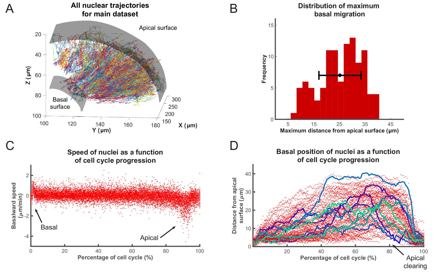
Analysis of nuclear tracks during IKNM.
(A) Extracted trajectories of nuclei in three dimensions. All curated tracks of the main data set over 400 min in the region shown in Figure 1C are presented. (B) The distribution of maximum distances reached away from the apical surface by nuclei during their completed cell cycles. The mean and one standard deviation are shown. (C) The speed distribution of 106 nuclei over complete cell cycles. The cell cycle lengths of all nuclei were normalized and superimposed to highlight the early basal burst of speed, as well as pre-division apical rapid migration. The speeds between these two periods are normally distributed. (D) Position of the same nuclei as in (C) measured by their distance from the apical surface over normalized cell cycle time. Even though all nuclei start and end their cell cycle near the apical surface, they move out across the retina to take positions in all available spaces, creating an apical clearing as indicated. Tracks for 10 randomly chosen nuclei are shown as colored lines to highlight the variability in the traversed trajectories.
Figure 3
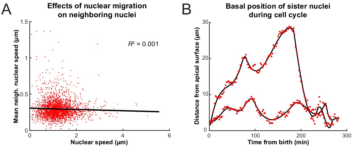
Interactions of nuclei in close proximity.
(A) Average speed of nuclei neighboring a nucleus of interest as a function of the speed of that nucleus. (B) The positions of two sister nuclei at each time point imaged (red circles) over their complete cell cycle. The black lines are spline curves indicating the general trend of their movements.
Figure 4
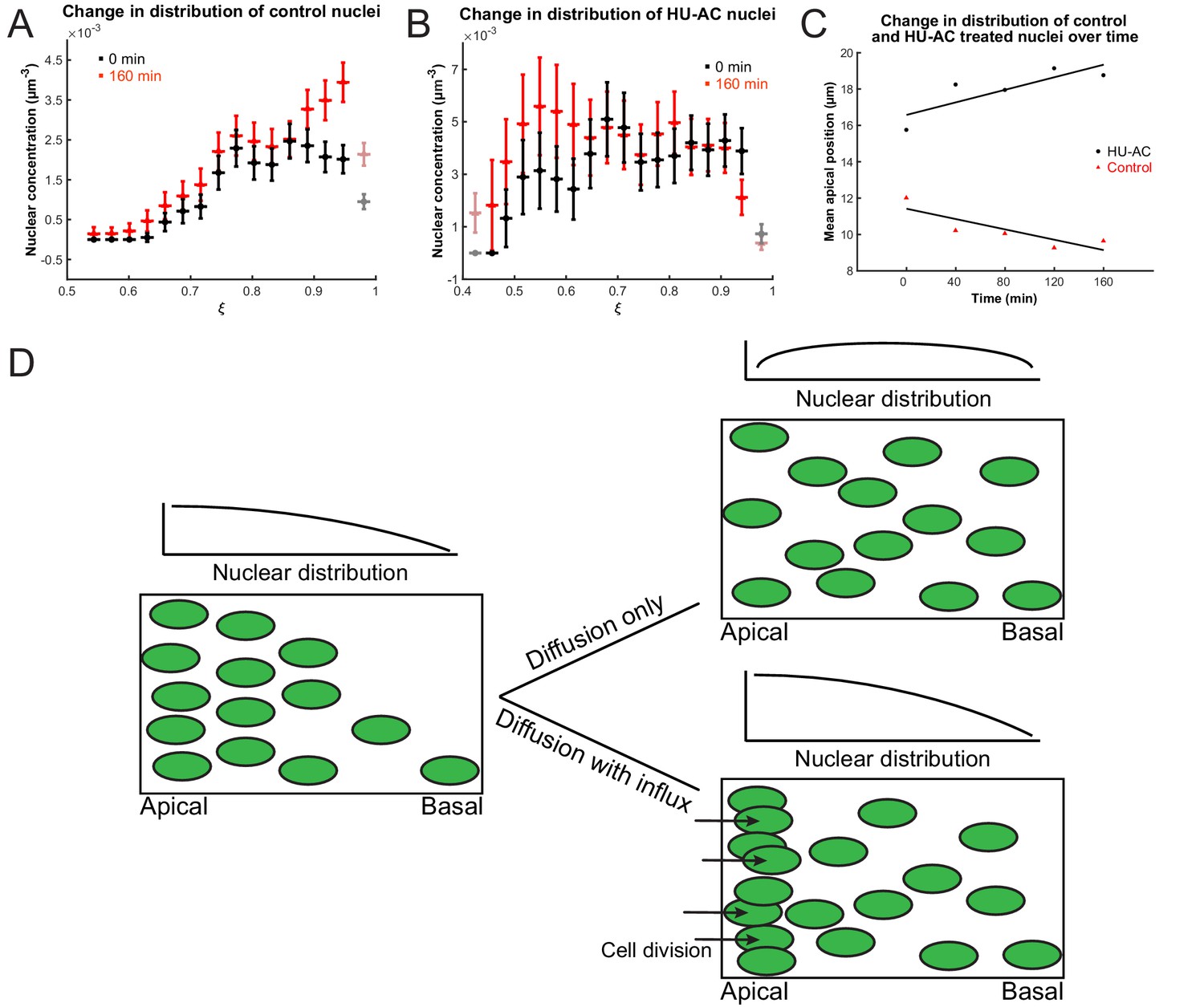
Nuclear concentration gradient across the apicobasal axis of the retina.
The concentration of nuclei is higher near the apical surface compared to the basal surface. (A) In the control retina, the nuclear concentration gradient builds up over time. (B) Blocking apical migration and division of nuclei, by inhibiting S phase progression, leads to a shift in the distribution of nuclei toward the basal surface in the HU-AC treated retina. In A and B, the coordinate is used, where a is the radius of the apical surface and r the distance from the center of the lens. (C) The shift in the distribution of nuclei under HU-AC treatment when compared to the untreated retina. The average distance of nuclei away from the apical surface increases consistently over time in the absence of cell division, but remains the same when new nuclei are constantly added at the apical surface. (D) A schematic of how a diffusion model would work in the context of IKNM in the retina. A concentration gradient of nuclei (left) would drive the net movement of nuclei from the apical surface to the basal surface. However, without maintenance of the gradient, the drive for this net migration is lost (top right). In the retina, the gradient is maintained through cell divisions at the apical surface, modeled as a one-way influx across the apical surface (bottom right), continuously driving the net movement basally.
Figure 5
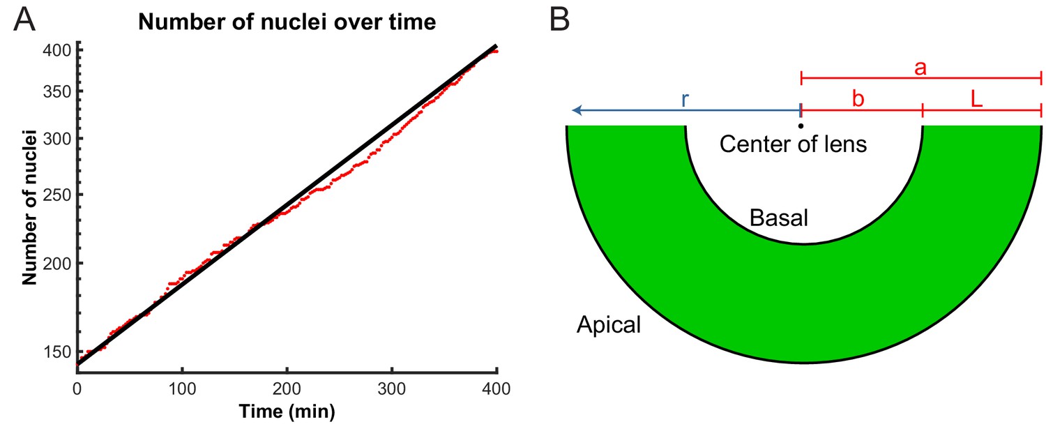
Model parameters extracted from experimental data.
(A) Number of nuclei grows exponentially during the proliferative stage of the retinal development. A line can be fitted to the log-lin graph of nuclear numbers as a function of time to extract the doubling time (cell cycle length) in this period. (B) A schematic of the retina indicating the variables used in the diffusion model of IKNM. a: distance from center of lens to apical surface; b: distance from center of lens to basal surface; L: thickness of the retina; r: distance from center of lens for each particle.
Figure 6
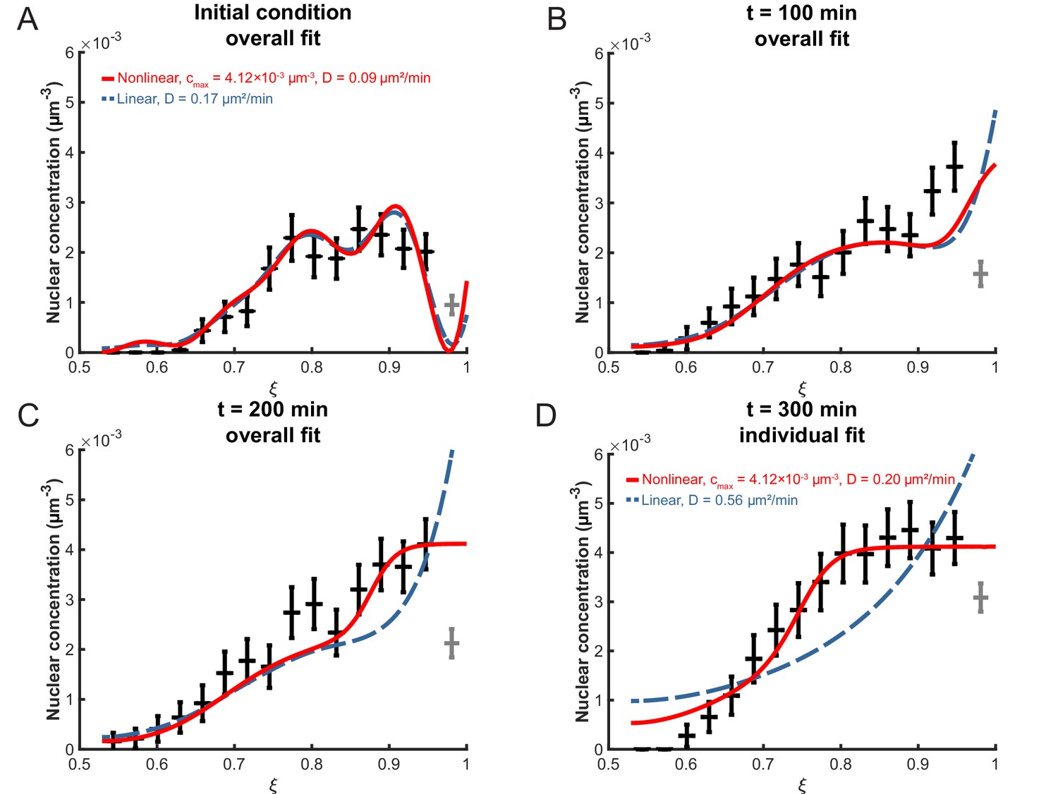
Fitting the linear and nonlinear models to the distribution of nuclei over time.
(A) The initial experimental concentration profile of nuclei at min, as well as the calculated initial condition curves (see Materials and methods Equation 17) for the linear (red solid line) and nonlinear (blue dashed line) models. The fit of the models to experimental distribution of nuclei after 100 min (B), 200 min (C), and 300 min (D) are shown. For the first three graphs, the best fits over all 100 intervening time points were used with the corresponding diffusion constants shown in (A). For t = 300 min, the best fits at that time point only were used with the corresponding diffusion constants indicated.
Figure 7

Cell shapes.
(A) Equilibrium cell shape obtained from minimization of elastic energy, with specified radii µm and µm at apical and basal sides. Here, the length L of the cell is taken to be 55 µm. (B) Coordinate system defined in Daniels, 2019, where is the nuclear radius and and θ are the radius of the membrane tube around the nucleus and the opening angle of the membrane, respectively.
Figure 8
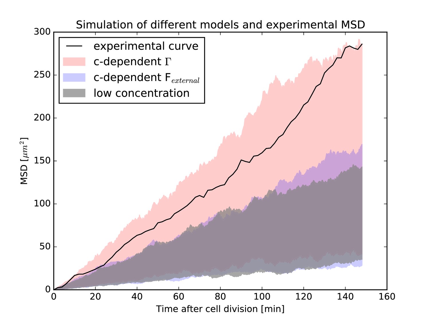
Mean-squared-displacement (MSD) of the first 40 nuclei that could be tracked beginning with cell division in the experiment.
The black curve is the experimental MSD curve as a function of (cell-internal) time after cell division. The shaded areas represent the simulations of different models. In red is the model that assumes the effect of surrounding nuclei is due to a concentration dependence of the stochastic force (i.e. has a concentration-dependent ). In blue is the model that includes the effect of surrounding nuclei via an additional force . In gray is the model for low nuclear concentration for comparison. In each case, the same 40 nuclei as the experiment have been simulated, taking their respective environment (i.e. the surrounding nuclear concentration) into account. In each simulation, the MSD curve was calculated as in the experiment. For each model, simulations were repeated 2500 times and the shaded areas represent the range of values covered by the individual resulting MSD curves for each model. The experimental MSD curve only agrees with the model assuming a concentration-dependent stochastic force.
Tables
Table 1
List of best-fit diffusion constants , their standard deviations and probabilities for the studied conditions.
| (µm2/min) | (µm2/min) | ||
|---|---|---|---|
| Normal | 0.09 | 0.05 | 0.49–0.51 |
| Normal (repeat sample) | 0.10 | 0.06 | 0.47–0.48 |
| High T | 0.13 | 0.08 | 0.42 |
| Low T | 0.06 | 0.05 | 0.69–0.7 |
Additional files
-
Source code 1
All track information for main data set.
The fields within this data structure are: fullTr: n x six matrix where n is the number of all nuclei within one lineage. In this matrix: column 1 - object ID at each time point; columns 2–4 - (x,y,z); column 5 - parent ID (=ID from previous time point); column 6 - time point (2 min per time point). indTracks: Separated, ”individual’ tracks of a lineage where each track starts at t = 0 or a division and ends at t = end or another division. Each cell in the array is a track and contains a matrix with only nuclei of that track (same columns as fullTr). distVel: The distance and velocity vector for each nucleus at each time point. Each row corresponds to distance and velocity of the nucleus going from that time point to the next. Each cell corresponds to the same one in indTracks. In the matrices: column 1 - time point; column 2 - distance (magnitude of velocity vector); column 3 - cumulative distance; columns 4–6 - velocity vector (x,y,z) corrIndTracks and corrDistVel: The exact same as indTracks and distVel, but corrected for drift. Correction was carried out by calculating the sum of all displacement vectors at each time point and then changing all position vectors in indTracks to make that sum zero, which gave us corrIndTracks. That was then used to calculate corrDistVel. As for the second column of cells in corrIndTracks, it relates to the neighbours of each nucleus. Each element of a cell in the second column stores the address of neighbours of the corresponding nucleus in the first column (address matrix: column 1 - Tracks row index; column 2 - corrIndTracks row index; column 3 - object row index). apBasProj: The projection of velocity vectors onto the calculated normals to the apical surface. In this matrix: column 1–3 - apicobasal velocity vector (x,y,z); column 4 - magnitude of the vector; column 5 - direction (negative = apical and positive = basal). lateralProj: The component of the velocity vectors perpendicular to the apicobasal one. Same columns as in apBasProj without column 5.
- https://cdn.elifesciences.org/articles/58635/elife-58635-code1-v1.mat.zip
-
Source code 2
Set of distances of all nuclei from the apical surface for each time point for the normal condition data set (this was originally extracted from Tracks.mat but used in this way for all the analysis of nuclear distribution or concentration).
The time points are every 2 min (including t = 0 min in the first column) except for the HUAC data set where they are every 40 min (including t = 0 min which is 120 min after drug treatment).
- https://cdn.elifesciences.org/articles/58635/elife-58635-code2-v1.mat.zip
-
Source code 3
Set of distances of all nuclei from the apical surface for each time point for the high temperature data set.
The time points are every 2 min (including t = 0 min in the first column) except for the HUAC data set where they are every 40 min (including t = 0 min which is 120 min after drug treatment).
- https://cdn.elifesciences.org/articles/58635/elife-58635-code3-v1.mat.zip
-
Source code 4
Set of distances of all nuclei from the apical surface for each time point for the low temperature data set.
The time points are every 2 min (including t = 0 min in the first column) except for the HUAC data set where they are every 40 min (including t = 0 min which is 120 min after drug treatment).
- https://cdn.elifesciences.org/articles/58635/elife-58635-code4-v1.mat.zip
-
Source code 5
Set of distances of all nuclei from the apical surface for each time point for the repeat normal condition data set.
The time points are every 2 min (including t = 0 min in the first column) except for the HUAC data set where they are every 40 min (including t = 0 min which is 120 min after drug treatment).
- https://cdn.elifesciences.org/articles/58635/elife-58635-code5-v1.mat.zip
-
Source code 6
Set of distances of all nuclei from the apical surface for each time point for the HU-AC treatment data set.
The time points are every 2 min (including t = 0 min in the first column) except for the HUAC data set where they are every 40 min (including t = 0 min which is 120 min after drug treatment).
- https://cdn.elifesciences.org/articles/58635/elife-58635-code6-v1.mat.zip
-
Transparent reporting form
- https://cdn.elifesciences.org/articles/58635/elife-58635-transrepform-v1.pdf
Download links
A two-part list of links to download the article, or parts of the article, in various formats.
Downloads (link to download the article as PDF)
Open citations (links to open the citations from this article in various online reference manager services)
Cite this article (links to download the citations from this article in formats compatible with various reference manager tools)
Nuclear crowding and nonlinear diffusion during interkinetic nuclear migration in the zebrafish retina
eLife 9:e58635.
https://doi.org/10.7554/eLife.58635


