Does diversity beget diversity in microbiomes?
- Département de sciences biologiques, Université de Montréal, Canada
- European Centre for Environment and Human Health, University of Exeter, United Kingdom
- Department of Microbiology and Immunology, McGill University, Canada
- McGill Genome Centre, McGill University, Canada
Figures
Figure 1
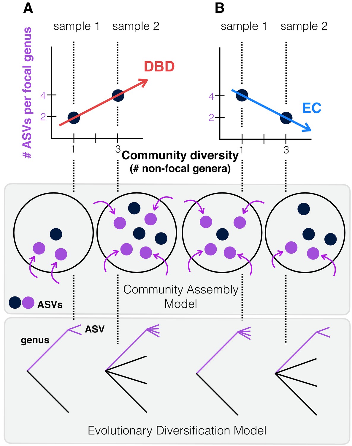
Contrasting the Diversity Begets Diversity (DBD) and Ecological Controls (EC) models.
(A). In this hypothetical scenario, microbiome sample 1 contains one non-focal genus, and two amplicon sequence variants (ASVs) within the focal genus (point at x = 1, y = 2 in the plot). Sample 2 contains three non-focal genera, and four ASVs within the focal genus (point at x = 3, y = 4). Tracing a line through these points yields a positive diversity slope, supporting the DBD model (red). (B) Alternatively, a negative slope would support the Ecological Controls (EC) model (blue line). In the middle panel, we consider a community assembly model to explain the hypothetical data of the top panel, in which standing diversity (black points) in a community selects (for or against) new types (referred to here as ASVs) which arrive via migration (purple points and arrows). In the bottom panel, we consider an evolutionary diversification model of a focal lineage (genus) into ASVs as a function of initial genus-level community diversity present at the time of diversification.
Figure 2 with 26 supplements
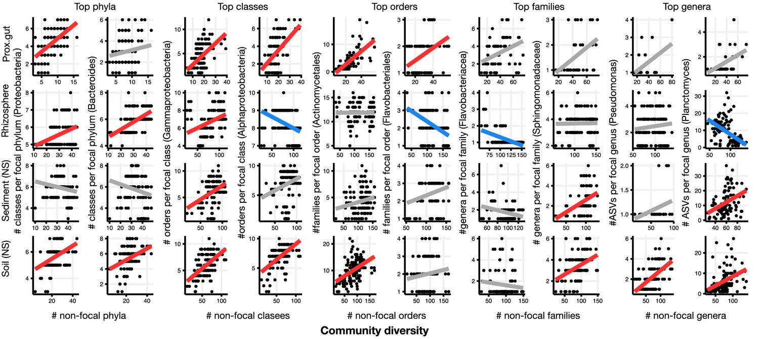
Focal-lineage diversity as a function of community diversity in the top two most prevalent taxa at each taxonomic level.
As in Figure 1, the x-axes show community diversity in units of the number of non-focal taxa (e.g. the number of non-Proteobacteria phyla for the left-most column), and the y-axes show the taxonomic ratio within the focal taxon (e.g. the number of classes within Proteobacteria). Significant positive diversity slopes are shown in red, negative in blue (linear models, p<0.05, Bonferroni corrected for 17 tests), and non-significant in grey. Note that linear models are distinct from GLMMs, and are for illustrative purposes only. Four representative environments are shown (see Figure 2—figure supplement 2–16 for plots in all 17 environments).
Figure 2—figure supplement 1
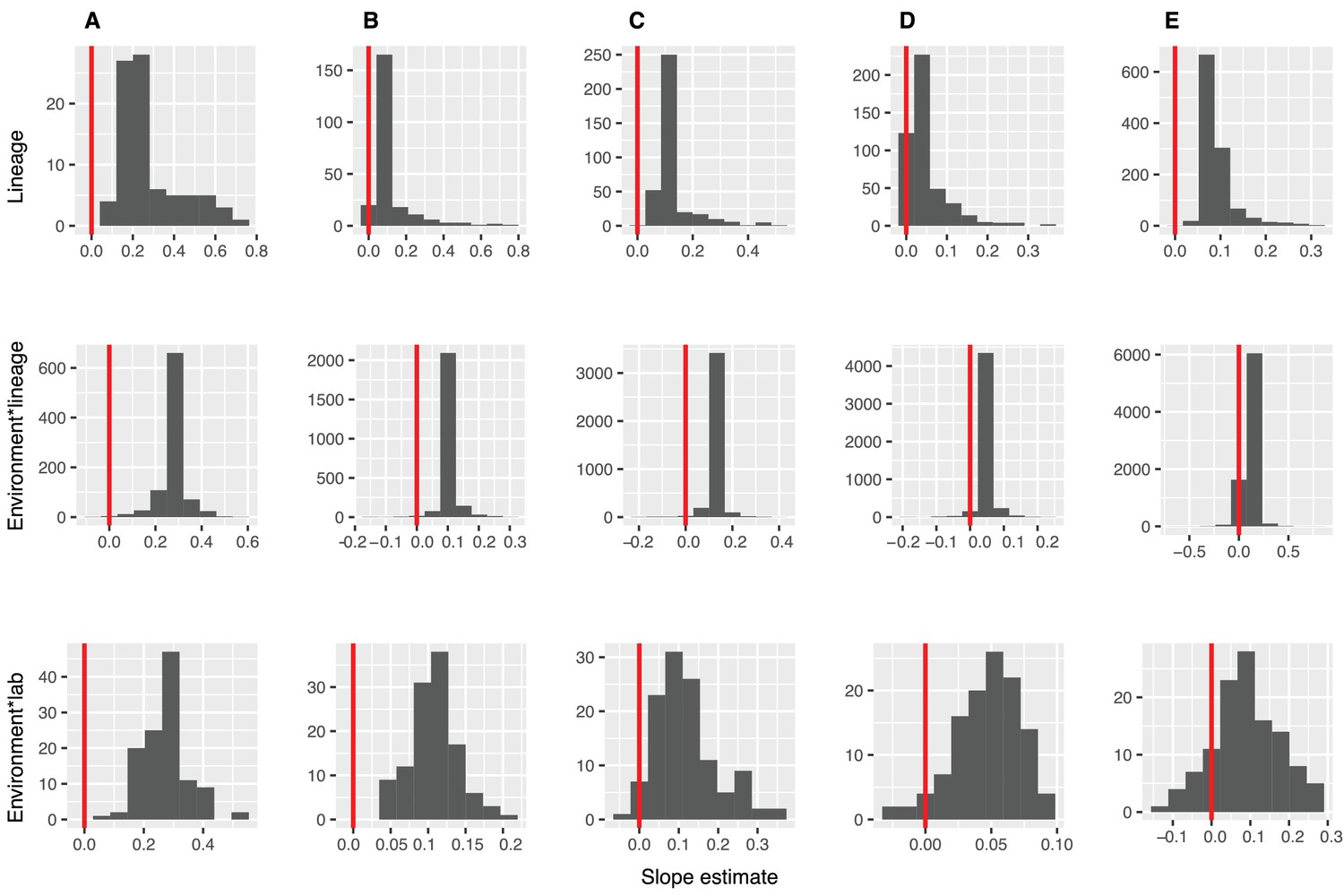
Distributions of diversity slope estimates across different random effects, from the GLMMs predicting focal lineage diversity as a function of community diversity.
(A) Class:Phylum, (B) Order:Class, (C) Family:Order, (D) Genus:Family, and (E) ASV:Genus. Estimation of random effect coefficients from the GLMMs (Table S1), shows that the effect of diversity on focal lineage diversity (slope estimates) are generally positive but could be negative in some lineages or combinations of environment, lineage (Environment*Lineage), and the laboratory that submitted the dataset (Environment*Lab).Linear models are shown for the number of classes per phylum (y-axis) as a function of community diversity (number of non-focal phyla, x-axis) in each of the 17 environments (EMPO3 biomes). Only environments containing the focal lineage are shown. P-values are Bonferroni corrected for 17 tests. Significant (p<0.05) models are shown with red trend lines.
Figure 2—figure supplement 2

Focal-lineage diversity as a function of community diversity across biomes in Proteobacteria.
Linear models are shown for the number of classes per phylum (y-axis) as a function of community diversity (number of non-focal phyla, x-axis) in each of the 17 environments (EMPO3 biomes). Only environments containing the focal lineage are shown. P-values are Bonferroni corrected for 17 tests. Significant (p<0.05) models are shown with red trend lines.
Figure 2—figure supplement 3
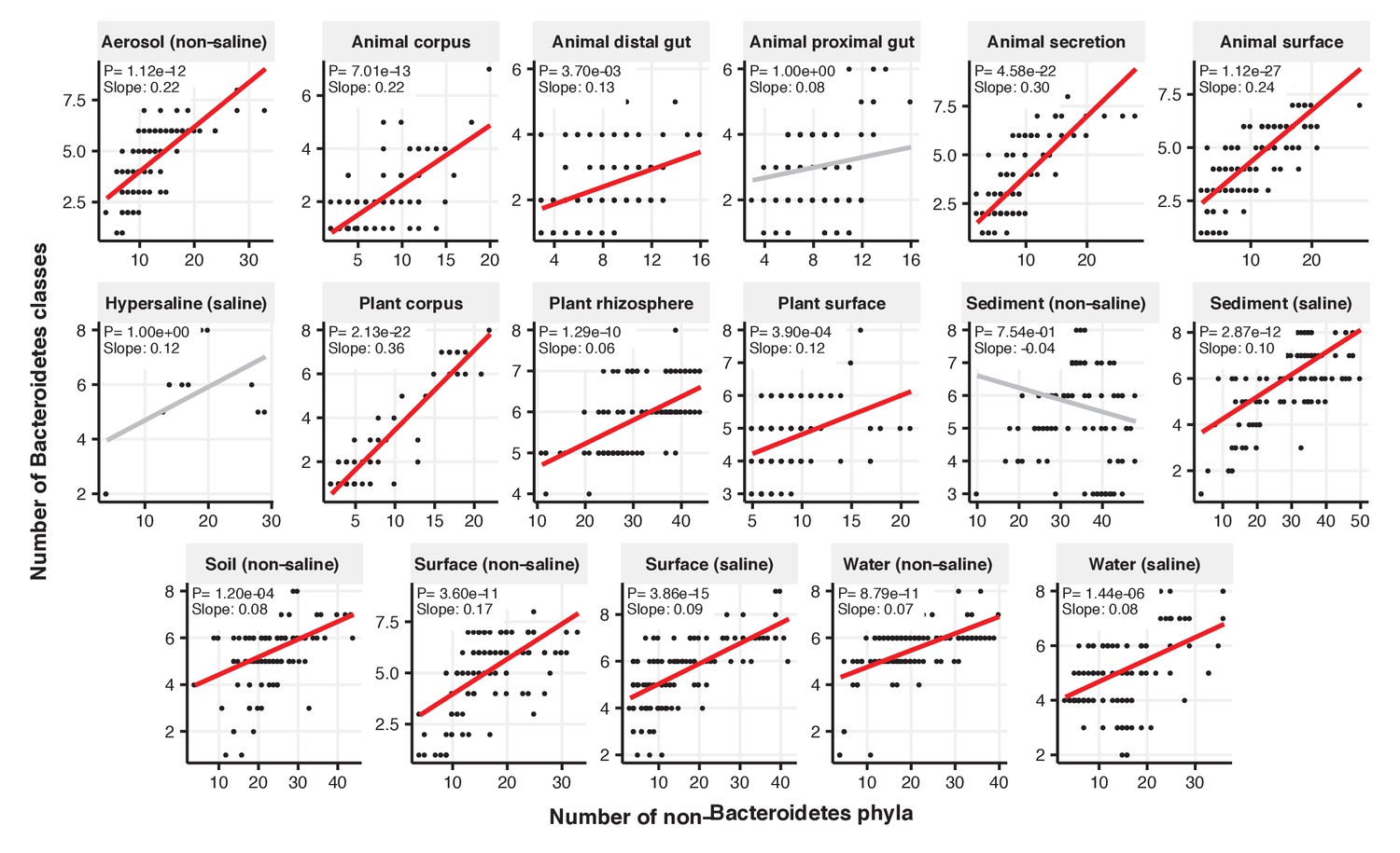
Focal-lineage diversity as a function of community diversity across biomes in Bacteroidetes.
Linear models are shown for the number of classes per phylum (y-axis) as a function of community diversity (number of non-focal phyla, x-axis) in each of the 17 environments (EMPO3 biomes). Only environments containing the focal lineage are shown. P-values are Bonferroni corrected for 17 tests. Significant (p<0.05) models are shown with red trend lines.
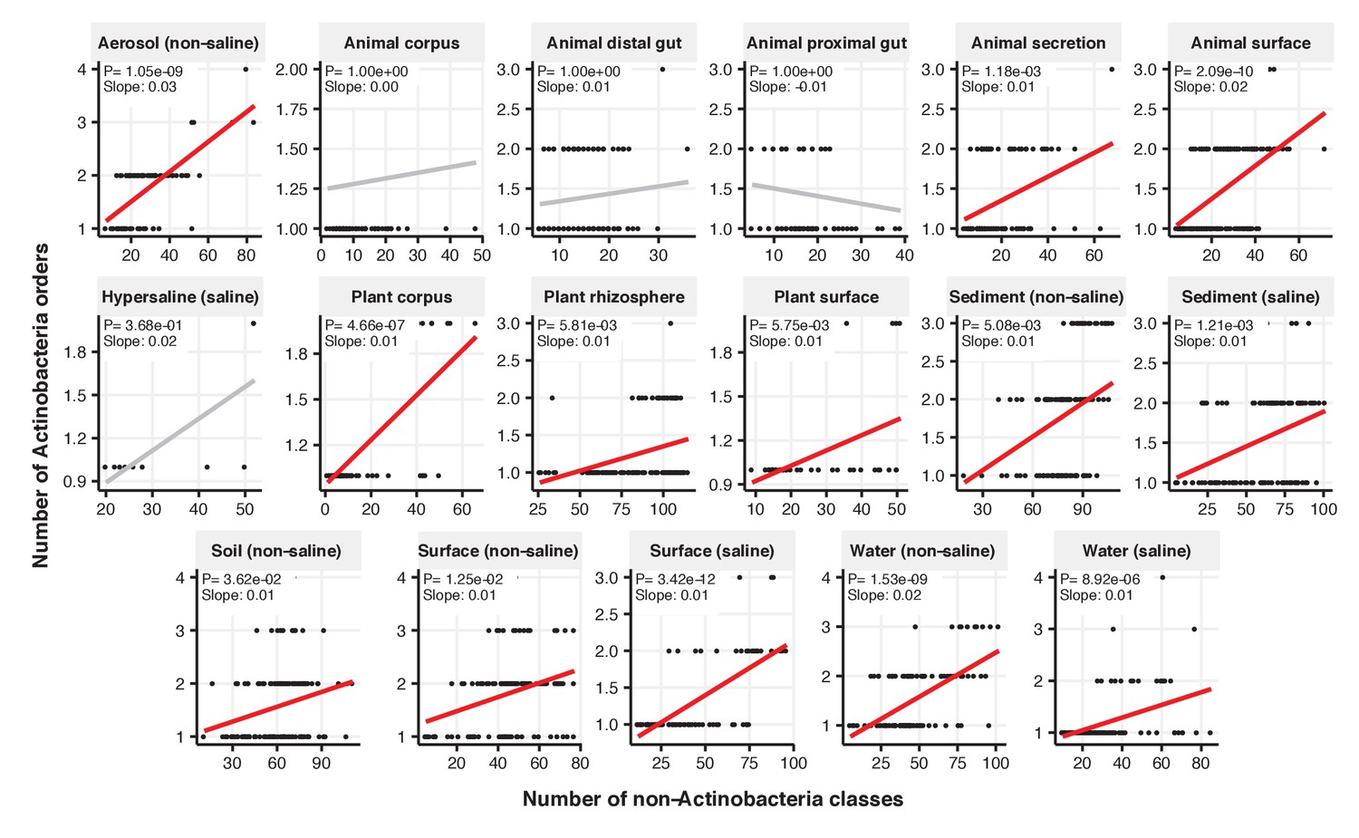
Figure 2—figure supplement 4
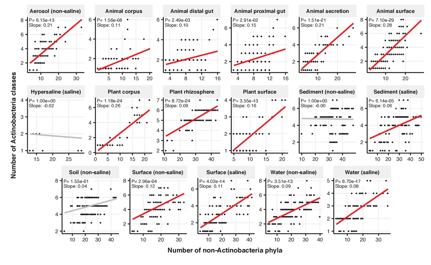
Focal-lineage diversity as a function of community diversity across biomes in Actinobacteria.
Linear models are shown for the number of classes per phylum (y-axis) as a function of community diversity (number of non-focal phyla, x-axis) in each of the 17 environments (EMPO3 biomes). Only environments containing the focal lineage are shown. P-values are Bonferroni corrected for 17 tests. Significant (p<0.05) models are shown with red trend lines.
Figure 2—figure supplement 5
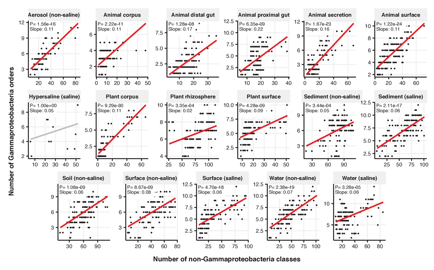
Focal-lineage diversity as a function of community diversity across biomes in Gammaproteobacteria.
Linear models are shown for the number of orders per class (y-axis) as a function of community diversity (non-focal classes, x-axis) in each of the 17 environments (EMPO3 biomes). Only environments containing the focal lineage are shown. Significant positive diversity slopes are shown in red (linear models, p<0.05, Bonferroni corrected for 17 tests), and non-significant in grey.
Figure 2—figure supplement 6

Focal-lineage diversity as a function of community diversity across biomes in Alphaproteobacteria.
Linear models are shown for the number of orders per class (y-axis) as a function of community diversity (non-focal classes, x-axis) in each of the 17 environments (EMPO3 biomes). Only environments containing the focal lineage are shown. Significant positive diversity slopes are shown in red, negative in blue (linear models, p<0.05, Bonferroni corrected for 17 tests), and non-significant in grey.
Figure 2—figure supplement 7
Focal-lineage diversity as a function of community diversity across biomes in Actinobacteria.
Linear models are shown for the number of orders per class (y-axis) as a function of community diversity (non-focal classes, x-axis) in each of the 17 environments (EMPO3 biomes). Only environments containing the focal lineage are shown. Significant positive diversity slopes are shown in red (linear models, p<0.05, Bonferroni corrected for 17 tests), and non-significant in grey.
Figure 2—figure supplement 8
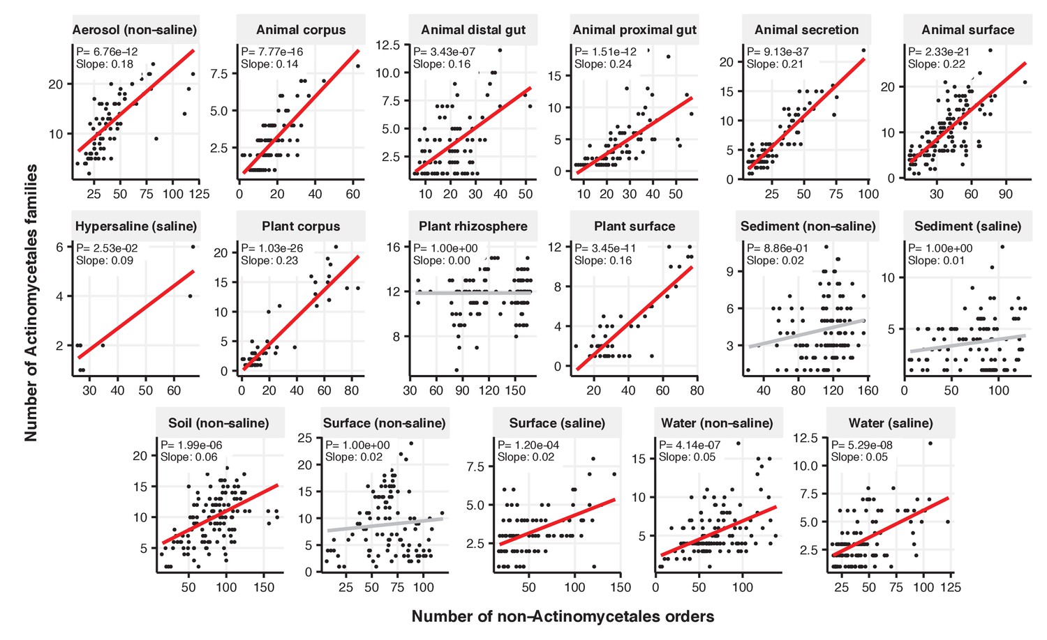
Focal-lineage diversity as a function of community diversity across biomes in Actinomycetales.
Linear models are shown for the number of families per order (y-axis) as a function of community diversity (non-focal orders, x-axis) in each of the 17 environments (EMPO3 biomes). Only environments containing the focal lineage are shown. Significant positive diversity slopes are shown in red (linear models, p<0.05, Bonferroni corrected for 17 tests), and non-significant in grey.
Figure 2—figure supplement 9

Focal-lineage diversity as a function of community diversity across biomes in Flavobacteriales.
Linear models are shown for the number of families per order (y-axis) as a function of community diversity (non-focal orders, x-axis) in each of the 17 environments (EMPO3 biomes). Only environments containing the focal lineage are shown. Significant positive diversity slopes are shown in red, negative in blue (linear models, p<0.05, Bonferroni corrected for 17 tests), and non-significant in grey.
Figure 2—figure supplement 10
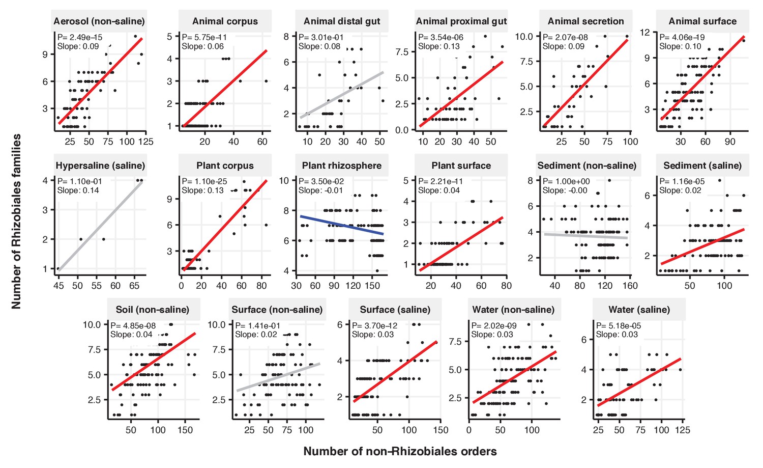
Focal-lineage diversity as a function of community diversity across biomes in Rhizobiales.
Linear models are shown for the number of families per order (y-axis) as a function of community diversity (non-focal orders, x-axis) in each of the 17 environments (EMPO3 biomes). Only environments containing the focal lineage are shown. Significant positive diversity slopes are shown in red, negative in blue (linear models, p<0.05, Bonferroni corrected for 17 tests), and non-significant in grey.
Figure 2—figure supplement 11

Focal-lineage diversity as a function of community diversity across biomes in Flavobacteriaceae.
Linear models are shown for genera per family (y-axis) as a function of community diversity (non-focal families, x-axis) in each of the 17 environments (EMPO3 biomes). Only environments containing the focal lineage are shown. Significant positive diversity slopes are shown in red, negative in blue (linear models, p<0.05, Bonferroni corrected for 17 tests), and non-significant in grey.
Figure 2—figure supplement 12
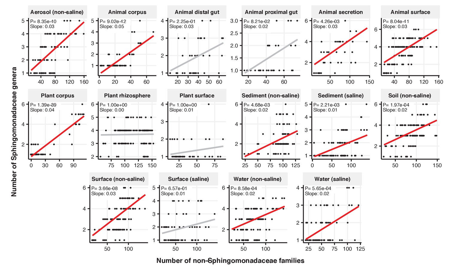
Focal-lineage diversity as a function of community diversity across biomes in Sphingomonadaceae.
Linear models are shown for genera per family (y-axis) as a function of community diversity (non-focal families, x-axis) in each of the 17 environments (EMPO3 biomes). Only environments containing the focal lineage are shown. Significant positive diversity slopes are shown in red (linear models, p<0.05, Bonferroni corrected for 17 tests), and non-significant in grey.
Figure 2—figure supplement 13
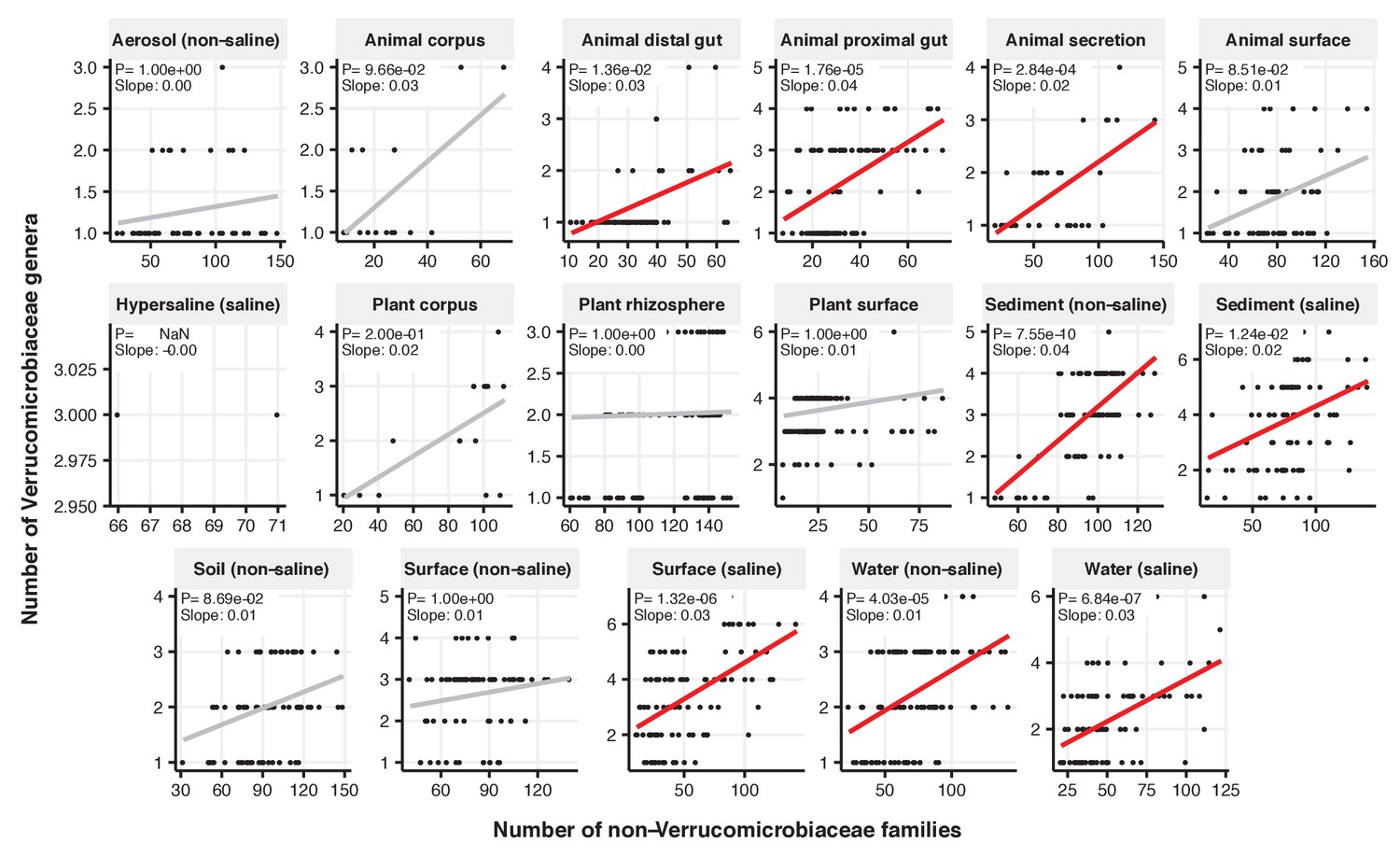
Focal-lineage diversity as a function of community diversity across biomes in Verrucomicrobiaceae.
Linear models are shown for genera per family (y-axis) as a function of community diversity (non-focal families, x-axis) in each of the 17 environments (EMPO3 biomes). Only environments containing the focal lineage are shown. Significant positive diversity slopes are shown in red (linear models, p<0.05, Bonferroni corrected for 17 tests), and non-significant in grey.
Figure 2—figure supplement 14
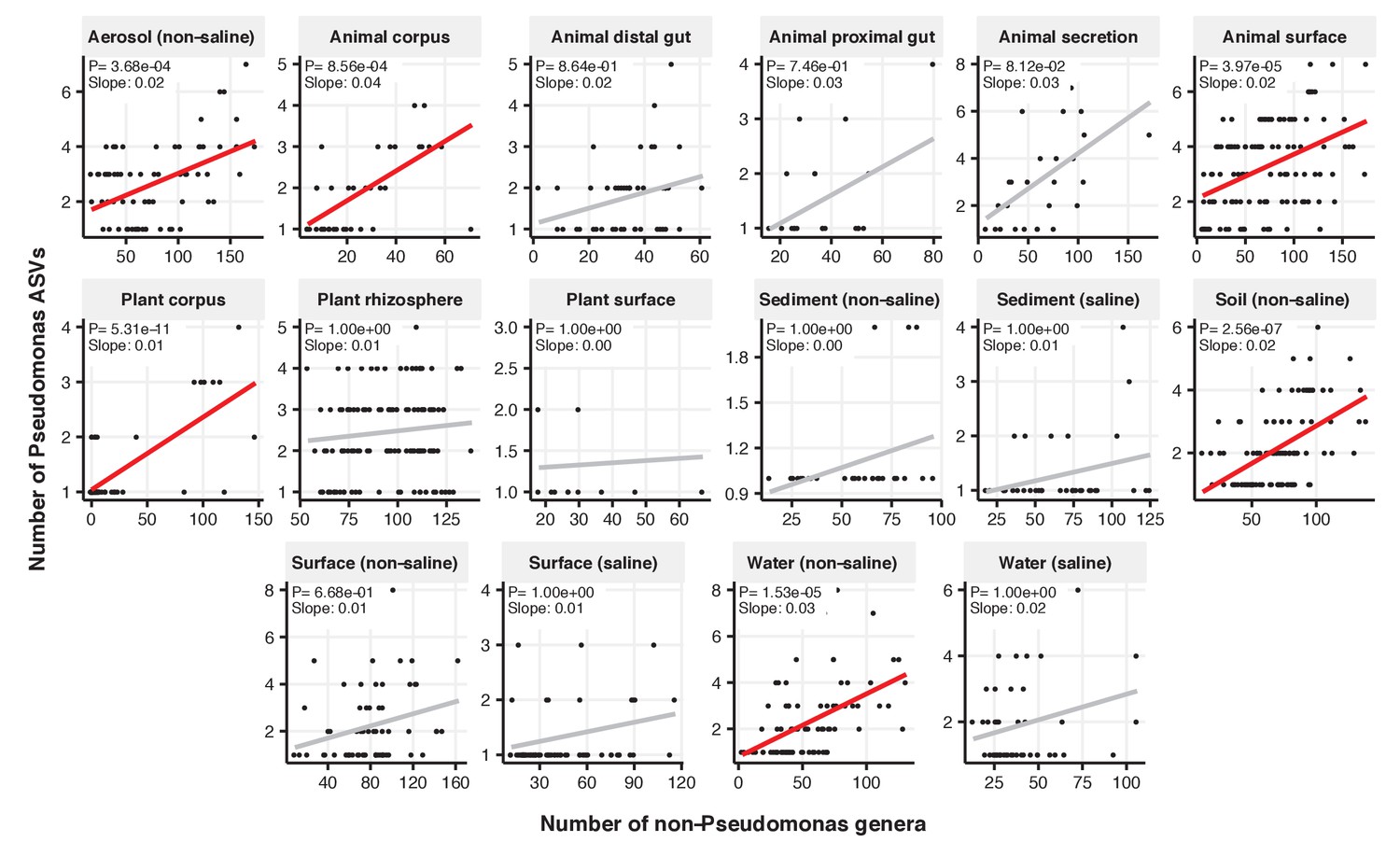
Focal-lineage diversity as a function of community diversity across biomes in Pseudomonas.
Linear models are shown for ASVs per genus (y-axis) as a function of community diversity (non-focal genera, x-axis) in each of the 17 environments (EMPO3 biomes). Only environments containing the focal lineage are shown. Significant positive diversity slopes are shown in red (linear models, p<0.05, Bonferroni corrected for 17 tests), and non-significant in grey.
Figure 2—figure supplement 15
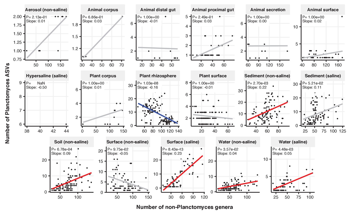
Focal-lineage diversity as a function of community diversity across biomes in Planctomyces.
Linear models are shown for ASVs per genus (y-axis) as a function of community diversity (non-focal genera, x-axis) in each of the 17 environments (EMPO3 biomes). Only environments containing the focal lineage are shown. Significant positive diversity slopes are shown in red, negative in blue (linear models, p<0.05, Bonferroni corrected for 17 tests), and non-significant in grey.
Figure 2—figure supplement 16
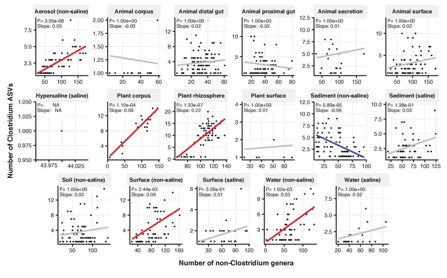
Focal-lineage diversity as a function of community diversity across biomes in Clostridium.
Linear models are shown for ASVs per genus (y-axis) as a function of community diversity (non-focal genera, x-axis) in each of the 17 environments (EMPO3 biomes). Only environments containing the focal lineage are shown. Significant positive diversity slopes are shown in red, negative in blue (linear models, p<0.05, Bonferroni corrected for 17 tests), and non-significant in grey.
Figure 2—figure supplement 17
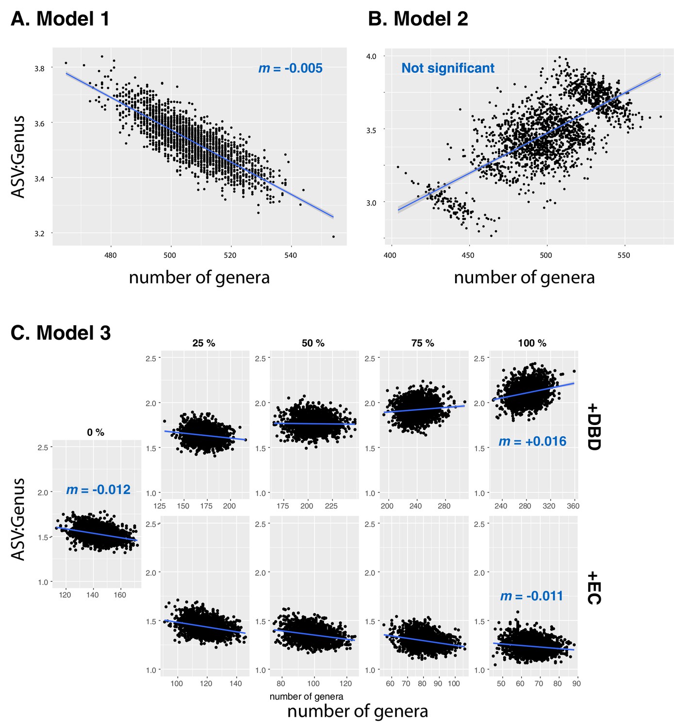
Null models based on Neutral Theory.
Results are shown from data simulated under (A) neutral Model 1, (B) neutral Model 2, or (C) neutral Model 3. Model 1 is sampled from the zero-sum multinomial distribution with a single distribution for the whole dataset, while Model 2 includes a separate distribution for each of the 17 different environments (EMPO 3 biomes). In Model 3 (C), the effect of DBD (top rows) or EC (bottom rows) are ‘spiked in’ at different levels, ranging from 0 to 100% of ASVs in a sample. Blue lines show a linear fit, with slopes (m) estimated by GLMM in selected panels. See Methods for model details, and Table 2 and Supplementary file 3, Section 1.2 for full GLMM results.
Figure 2—figure supplement 18

Lineage diversity (mean ASV:Genus ratio among all lineages) as a function of community diversity (number of genera) in the EMP data.
Samples from different environments (EMPO level 3) are shown in different colours, each with their corresponding linear model fit.
Figure 2—figure supplement 19
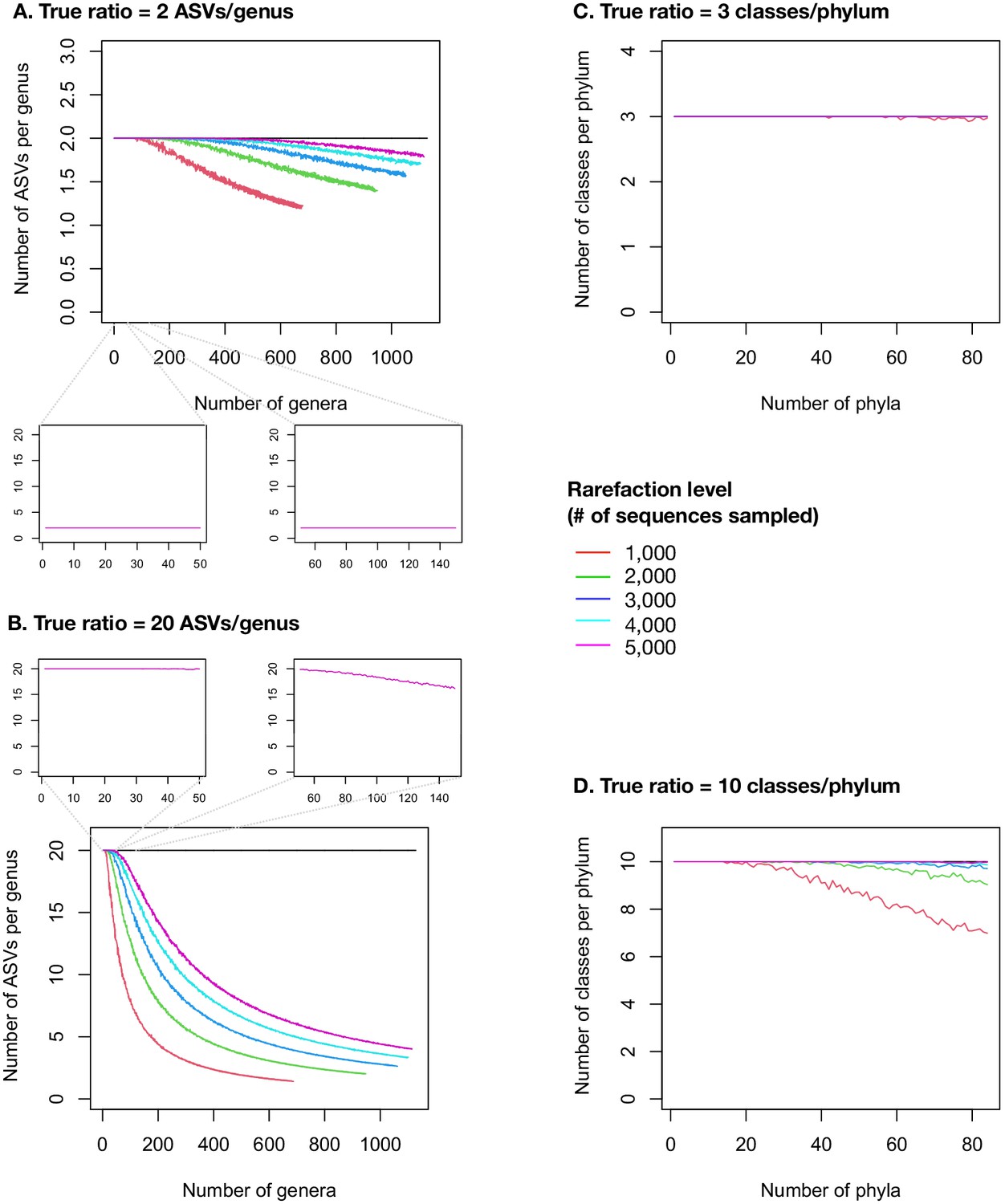
Taxonomic ratios estimated from simulated rarefied sequence data.
Each panel simulates a set of microbiome samples that differ in their diversity (number of genera in left panels A and B, number of phyla in right panels C and D) while maintaining a set true taxonomic ratio (horizontal black line). (A) True ratio set to 2 ASVs/genus, close to the per-sample mean and median in the real EMP data, in a range of samples between 1 and 1128 named genera, as observed in the real EMP data. (B) True ratio set to 20 ASVs/genus, equal to the overall mean of 22,014 named ASVs in 1128 named genera, and close to the maximum ratios observed in individual samples (Figure 2—figure supplement 5). Insets show the ranges of 1–50 and 51–150 genera, approximating observations from lower- or higher-diversity samples such as gut and soil, respectively (Figure 2—figure supplement 5). The insets only show the rarefaction to 5000 sequences, as used in the real EMP dataset. (C) True ratio set to three classes/phylum, close to the per-sample mean and median in the real EMP data, in a range of samples between 1 and 84 named phyla, as observed in the real EMP data. (D) True ratio set to 10 classes/phylum, close to the maximum ratios observed in individual samples (Figure 2—figure supplements 2–4). Different rarefaction levels are shown as different coloured lines.
Figure 2—figure supplement 20
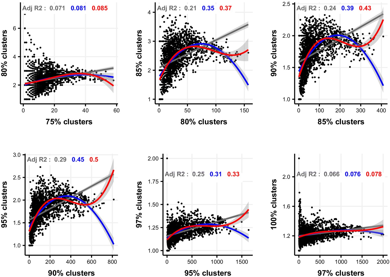
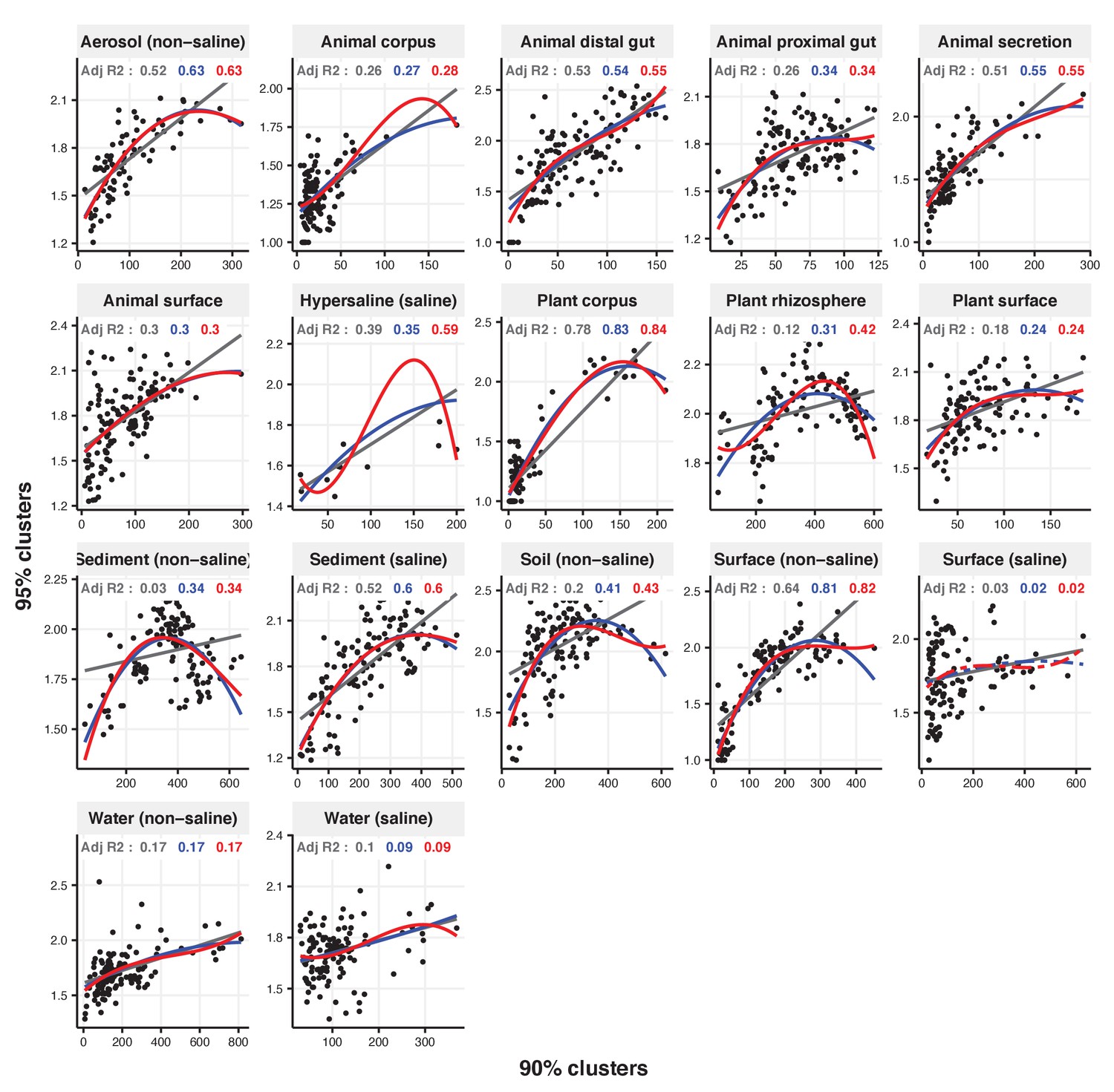
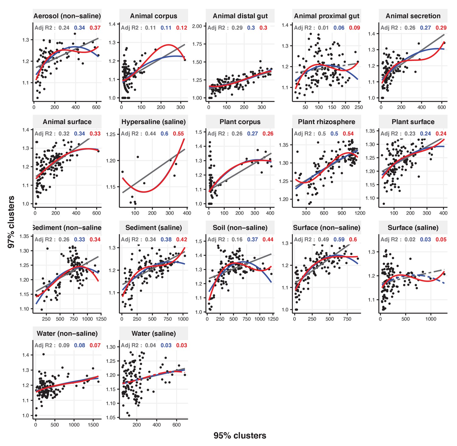
Linear, quadratic, and cubic models for the relationship between focal-lineage diversity and community diversity for varying levels of % nucleotide identity.
Community diversity was estimated as the number of clusters at a focal level (di) and focal-lineage diversity as the mean of the clusters at the rank above (di 1/di). All P-values are <0.001. Linear fit (grey); quadratic fit (blue), cubic fit (red); same colours for the associated adjusted R2. The x-axis (diversity) shows the number of clusters at the focal percent-identity level (di), and the y-axis (diversification) is the mean of the clusters at the rank above (di 1/di).
Figure 2—figure supplement 21
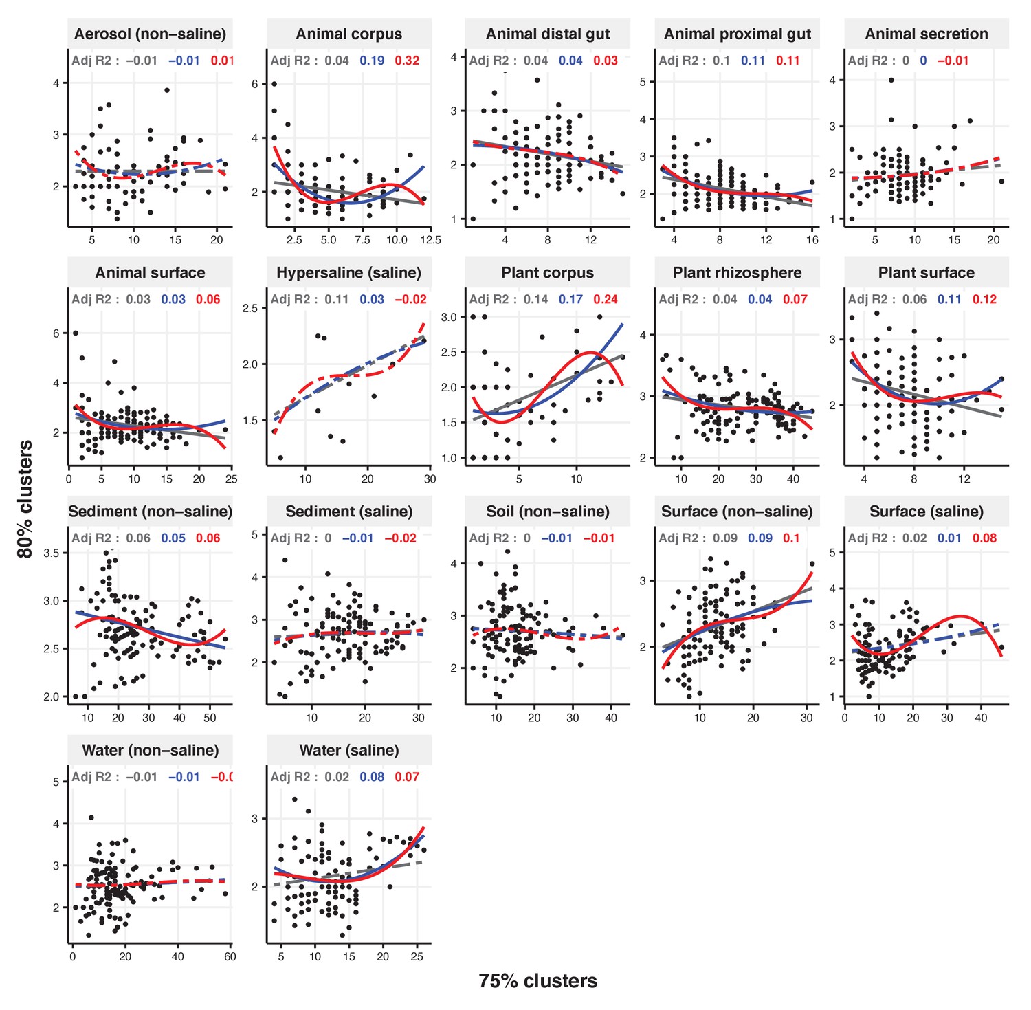
Focal clusters at 75% nucleotide identity.
Community diversity was estimated as the number of clusters at a focal level (di) and focal lineage diversity as the mean of the clusters at the rank above (di 1/di). Linear (grey), quadratic (blue) and cubic (red), with corresponding adjusted R-squared values in the same colour. P-values are Bonferroni corrected for 17 tests. Significant, p<0.05 (solid lines), non-significant (dashed lines). The x-axis shows the number of clusters at the focal percent-identity level (di), and the y-axis is the mean of the clusters at the rank above (di 1/di).
Figure 2—figure supplement 22
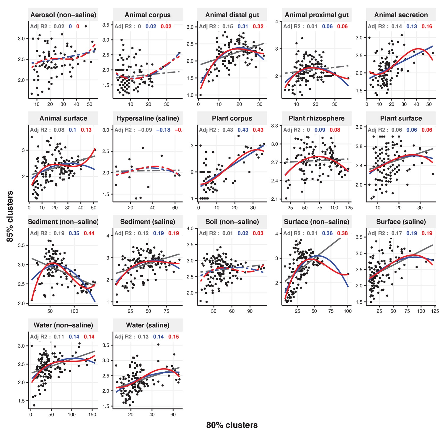
Focal clusters at 80% nucleotide identity.
Community diversity was estimated as the number of clusters at a focal level (di) and focal lineage diversity as the mean of the clusters at the rank above (di 1/di). Linear (grey), quadratic (blue) and cubic (red), with corresponding adjusted R-squared values in the same colour. P-values are Bonferroni corrected for 17 tests. Significant, p<0.05 (solid lines), non-significant (dashed lines). The x-axis shows the number of clusters at the focal percent-identity level (di), and the y-axis is the mean of the clusters at the rank above (di 1/di).
Figure 2—figure supplement 23
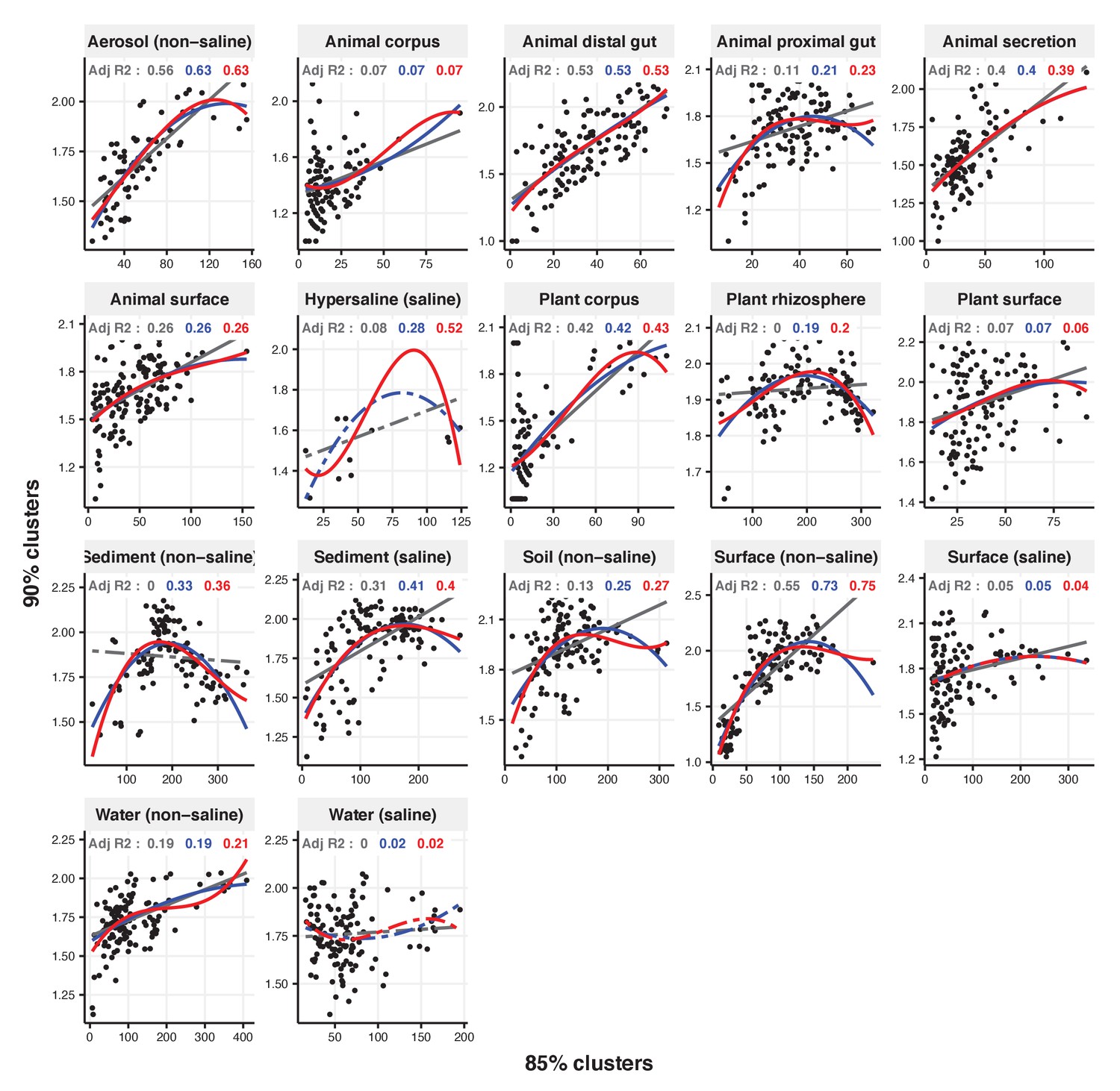
Focal clusters at 85% nucleotide identity.
Community diversity was estimated as the number of clusters at a focal level (di) and focal lineage diversity as the mean of the clusters at the rank above (di 1/di). Linear (grey), quadratic (blue) and cubic (red), with corresponding adjusted R-squared values in the same colour. P-values are Bonferroni corrected for 17 tests. Significant, p<0.05 (solid lines), non-significant (dashed lines). The x-axis shows the number of clusters at the focal percent-identity level (di), and the y-axis is the mean of the clusters at the rank above (di 1/di).
Figure 2—figure supplement 24
Focal clusters at 90% nucleotide identity.
Community diversity was estimated as the number of clusters at a focal level (di) and focal lineage diversity as the mean of the clusters at the rank above (di 1/di). Linear (grey), quadratic (blue) and cubic (red), with corresponding adjusted R-squared values in the same colour. P-values are Bonferroni corrected for 17 tests. Significant, p<0.05 (solid lines), non-significant (dashed lines). The x-axis shows the number of clusters at the focal percent-identity level (di), and the y-axis is the mean of the clusters at the rank above (di 1/di).
Figure 2—figure supplement 25
Focal clusters at 95% nucleotide identity.
Community diversity was estimated as the number of clusters at a focal level (di) and focal lineage diversity as the mean of the clusters at the rank above (di 1/di). Linear (grey), quadratic (blue) and cubic (red), with corresponding adjusted R-squared values in the same colour. P-values are Bonferroni corrected for 17 tests. Significant, p<0.05 (solid lines), non-significant (dashed lines). The x-axis shows the number of clusters at the focal percent-identity level (di), and the y-axis is the mean of the clusters at the rank above (di 1/di).
Figure 2—figure supplement 26
Focal clusters at 97% nucleotide identity.
Community diversity was estimated as the number of clusters at a focal level (di) and focal lineage diversity as the mean of the clusters at the rank above (di 1/di). Linear (grey), quadratic (blue) and cubic (red), with corresponding adjusted R-squared values in the same colour. P-values are Bonferroni corrected for 17 tests. Significant, p<0.05 (solid lines), non-significant (dashed lines). The x-axis shows the number of clusters at the focal percent-identity level (di), and the y-axis is the mean of the clusters at the rank above (di 1/di).
Figure 3
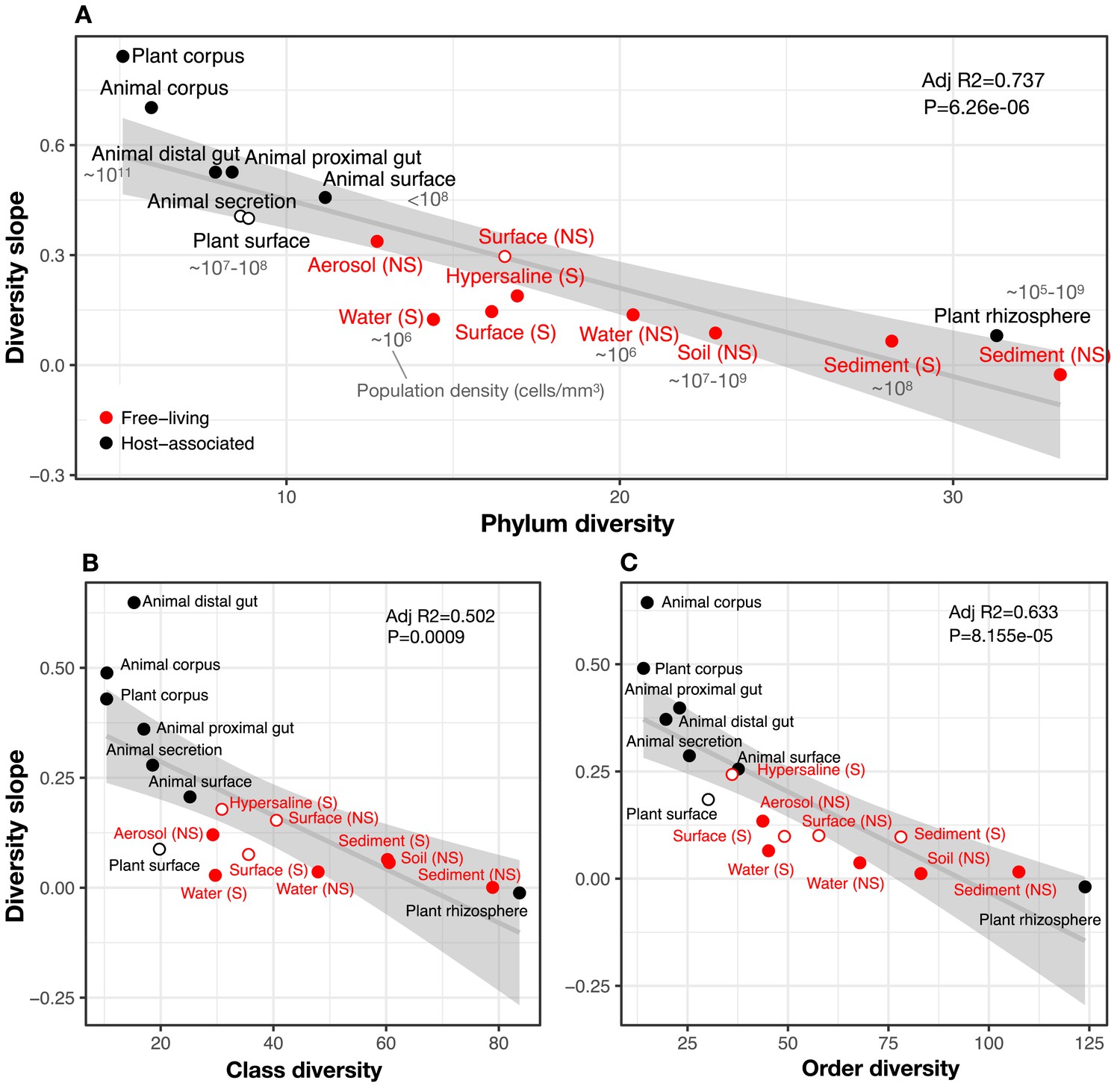
The diversity slope of focal taxa is higher in low-diversity (often host-associated) microbiomes.
The x-axis shows the mean number of non-focal taxa: (A) phyla, (B) classes, and (C) orders in each biome. On the y-axis, the diversity slope was estimated by a GLMM predicting focal lineage diversity as a function of the interaction between community diversity and environment type at the level of (A) Class:Phylum, (B) Order:Class, and (C) Family:Order ratios (Supplementary file 1 Section 3). The line represents a linear regression; the shaded area depicts 95% confidence limits of the fitted values. Adjusted R2 and P-values from the linear fits are shown at the top right of each panel. See Supplementary file 2 for model goodness of fit. Slopes not significantly different from zero are shown as empty circles. Estimates of bacterial cell density from the literature are indicated in grey text, in units of bacteria/mm3. For animal (skin) and plant surface, units of bacteria/mm2 were converted to mm3 assuming layers of bacteria one micron thick. For rhizosphere samples we assume a density of 1–2 g/cm3 (Kennedy and de Luna, 2005).
Figure 4 with 1 supplement
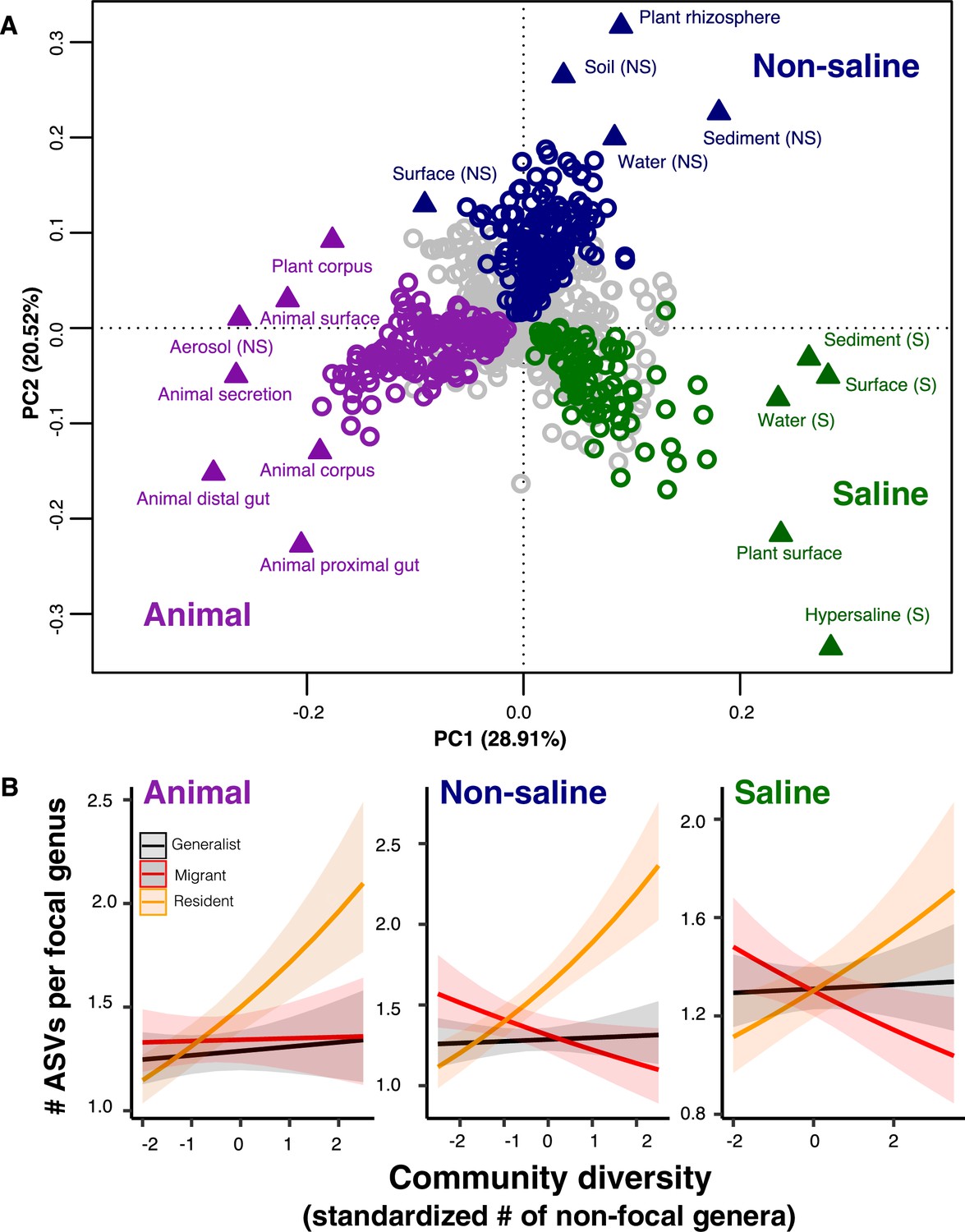
The DBD relationship varies between resident and non-resident genera.
(A) Ordination showing genera clustering into their preferred environment clusters. The matrix of 17 environments (rows) by 1128 genera (columns) by, with the matrix entries indicating the percentage of samples from a given environment in which each genus is present, was subjected to principal components analysis (PCA). Circles indicate genera and triangles indicate environments (EMPO 3 biomes). coloured circles are genera inferred by indicator species analysis to be residents of a certain environmental cluster, and grey circles are generalist genera. The three environment clusters identified by fuzzy k-means clustering are: Non-saline (NS, blue), saline (S, green) and animal-associated (purple). Triangles of the same colour indicate EMPO 3 biomes clustered into the same environmental cluster. (B) DBD in resident versus non-resident genera across environment clusters. Results of GLMMs modelling focal lineage diversity as a function of the interaction between community diversity and resident/migrant/generalist status. The x-axis shows the standardized number of non-focal resident genera (community diversity); the y-axis shows the number of ASVs per focal genus. Resident focal genera are shown in orange, migrant focal genera in red, and generalist focal genera in black. Red stars indicate a significantly positive or negative slope (Wald test, p<0.005). See Supplementary file 2 for model goodness of fit.
Figure 4—figure supplement 1
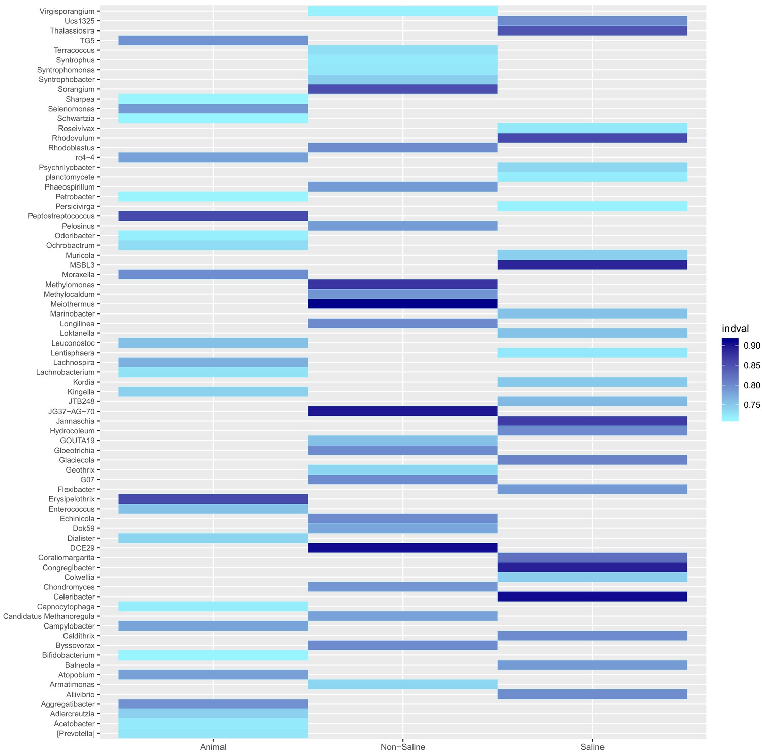
Resident genera of environment clusters.
Results from indicator species analysis illustrated as a heatmap. Only the 25 resident genera with the highest indval indices and p<0.05 (permutation test) are shown for every environment cluster (animal-associated, non-saline and saline free). For the full results see Supplementary file 5.
Figure 5
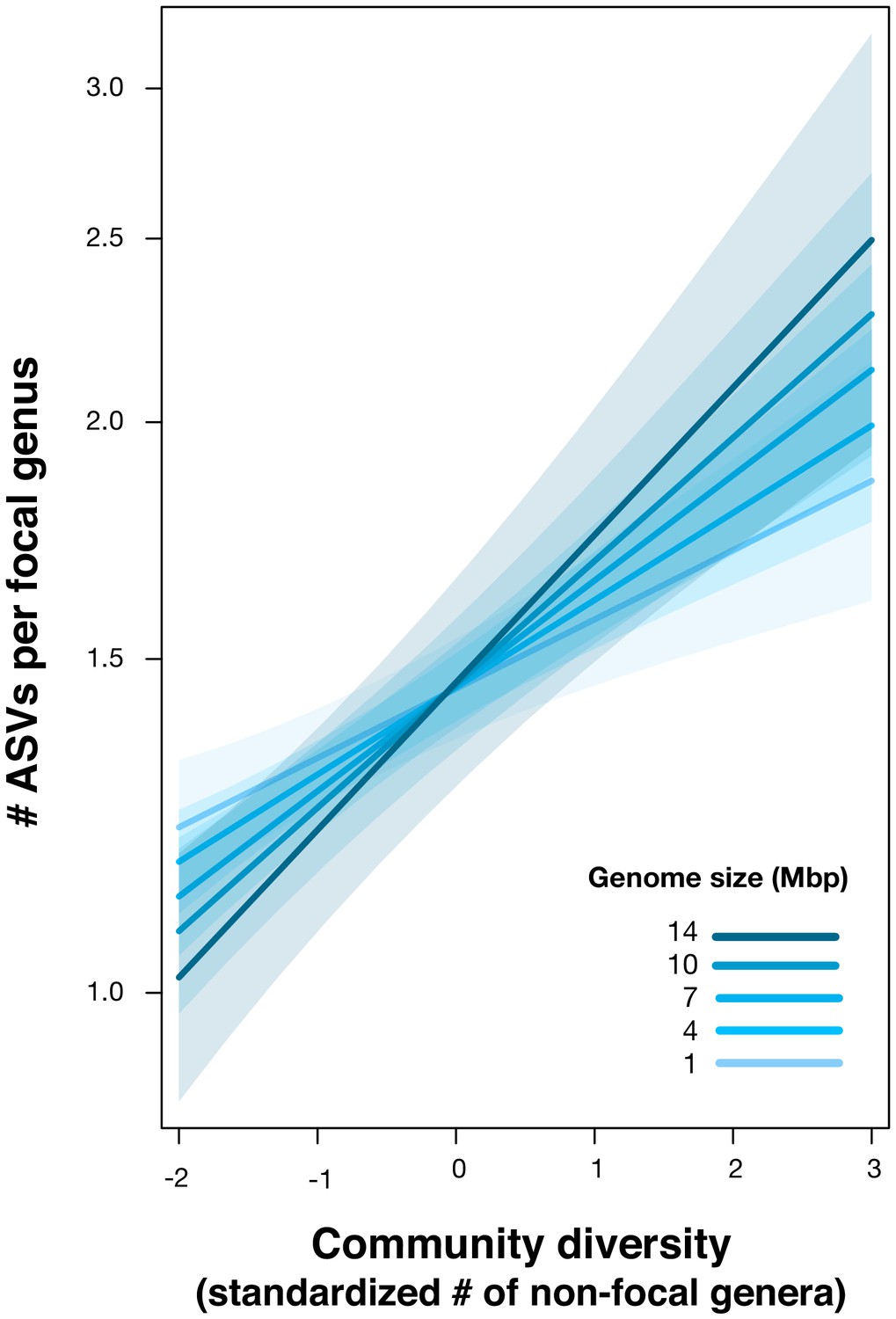
Positive effect of genome size on DBD.
Results are shown from a GLMM predicting focal lineage diversity as a function of the interaction between community diversity and genome size at the ASV:Genus ratio (Supplementary file 1 Section 6). The x-axis shows the standardized number of non-focal genera (community diversity); the y-axis shows the number of ASVs per focal genus. Variable diversity slopes corresponding to different genome sizes are shown in a blue colour gradient; the shaded area depicts 95% confidence limits of the fitted values. See Supplementary file 2 for model goodness of fit.
Tables
Table 1
Effects of community diversity on focal lineage diversity across taxonomic ratios.
The GLMMs show a statistically significant positive effect of community diversity on focal lineage diversity. Each row reports the effect of community diversity (Div) on focal lineage diversity, as well as its standard error, Wald z-statistic for its effect size and the corresponding P-value (left section), or standard deviation on the slope for the significant random effects (right section). SE = standard error, Env = environment type, Lin = lineage type, Lab = Principal Investigator ID, Sample = EMP Sample ID. Interactions are denoted as ‘*’. n.s. = not significant (likelihood-ratio test). All models provide a significantly better fit than null models without fixed effects (∆AIC > 10 and p<0.05; Supplementary file 2).
| Slope (fixed effects) | Standard deviation on the slope (random effects) | ||||||||
|---|---|---|---|---|---|---|---|---|---|
| Div | SE | z | P | Env | Lin | Lin*Env | Env*Lab | Sample | |
| ASV:Genus | 0.091 | 0.016 | 5.792 | 6.95e-09 | n.s. | 0.074 | 0.142 | 0.114 | 0.067 |
| Genus:Family | 0.047 | 0.008 | 5.911 | 3.41e-09 | n.s. | 0.071 | 0.07 | 0.039 | n.s. |
| Family:Order | 0.119 | 0.017 | 7.001 | 2.54e-12 | 0.023 | 0.094 | 0.092 | 0.106 | n.s. |
| Order:Class | 0.109 | 0.020 | 5.447 | 5.13e-08 | 0.05 | 0.141 | 0.078 | 0.051 | n.s. |
| Class:Phylum | 0.272 | 0.043 | 6.341 | 2.29e-10 | 0.119 | 0.174 | 0.119 | 0.114 | n.s. |
Table 2
GLMMs applied to data simulated under null models.
Null models 1 and 2 were generated under the ZSM distribution, with a single distribution for the whole dataset (Model 1) or one distribution per environment (Model 2). Model 3 is similar to Model 1, except with a single Poisson distribution for the whole dataset, and +DBD or +EC refer to adding these effects to all ASVs in each sample (see Materials and methods and Figure 2—figure supplement 17). Each row reports the effect of community diversity (Div) on focal lineage diversity, as well as its standard error, Wald z-statistic for its effect size and the corresponding P-value (Wald test) (left section), or standard deviation on the slope for the significant random effects (right section). SE = standard error, Env = environment type, Lin = lineage type, Sample = EMP Sample ID. n.s. = not significant (likelihood-ratio test), n.t. = not tested, because separate environments were not included in Models 1 or 3.
| Slope (fixed effects) | Stand dev on the slope (random effects) | |||||||
|---|---|---|---|---|---|---|---|---|
| Div | SE | z | P | Env | Lin | Lin*Env | Sample | |
| Model 1 | −0.005 | 0.000 | −9.807 | <2 e −16 | n.t. | 0.639 | n.t. | n.s. |
| Model 2 | n.s. | |||||||
| Model 3 | −0.012 | 0.002 | −6.552 | 5.69e-11 | n.t. | 0.021 | n.t. | n.s. |
| Model 3 + DBD | 0.016 | 0.001 | 11.48 | <2e-16 | n.t. | 0.008 | n.t. | n.s. |
| Model 3 + EC | −0.011 | 0.002 | −6.14 | 8.26e-10 | n.t. | ns | n.t. | n.s. |
Table 3
GLMMs with community diversity measured using Shannon diversity.
Results are shown from GLMMs with Shannon diversity of non-focal taxa (Div) as a predictor of ASVs richness of focal taxa. Each row reports the estimate (Div), as well as its standard error, Wald z-statistic for its effect size and the corresponding P-value (Wald test) (left section), or standard deviation on the slope for the significant random effects (right section). SE = standard error, Env = environment type, Lin = lineage type, Lab = Principal Investigator ID, Sample = EMP Sample ID. n.s. = not significant (likelihood-ratio test).
| Fixed effects | Random effects | ||||||||
|---|---|---|---|---|---|---|---|---|---|
| Div | SE | z | p | Env | Lin | Env*Lin | Env*Lab | Sample | |
| Genus | 0.055 | 0.013 | 4.33 | 1.49e-05 | n.s. | 0.08 | 0.15 | 0.085 | 0.054 |
| Family | 0.148 | 0227 | 6.491 | 8.51e-11 | n.s. | 0.184 | 0.268 | 0.16 | 0.134 |
| Order | 0.378 | 0.038 | 9.864 | <2e-16 | n.s. | 0.34 | 0.417 | 0.258 | 0.202 |
| Class | 0.398 | 0.05 | 7.973 | 1.54e-15 | n.s. | 0.369 | 0.46 | 0.326 | 0.262 |
| Phylum | 0.319 | 0.088 | 3.614 | 0.0003 | 0.169 | 0.316 | 0.5 | 0.495 | 0.378 |
Table 4
Community diversity has a stronger effect than abiotic factors on focal lineage diversity (EMP dataset).
Results are shown from GLMMs with community diversity (Div), four abiotic factors (temperature, elevation, pH, and latitude), and their interactions with community diversity, as predictors of focal lineage diversity. Random effects on the intercept included environment, lineage, lab ID and sample ID. Each row reports the taxonomic ratio, the predictors used in the GLMM (fixed effects only), their slope estimate (Est), standard error (SE) and P-value (P) (Wald test). Interactions are denoted as ‘*’. Random effects are not shown.
| Predictor | Est | SE | P | |
|---|---|---|---|---|
| ASV:Genus | Div | 0.128 | 0.013 | <2e-16 |
| Temperature | 0.04 | 0.014 | 0.00479 | |
| Div*Temperature | 0.043 | 0.014 | 0.00175 | |
| Div*Latitude | 0.031 | 0.013 | 0.02119 | |
| Div*Elevation | −0.031 | 0.014 | 0.02829 | |
| Genus:Family | Div | 0.094 | 0.009 | <2e-16 |
| Temperature | 0.026 | 0.009 | 0.00268 | |
| pH | −0.042 | 0.009 | 5.88e-06 | |
| Family:Order | Div | 0.131 | 0.01 | <2e-16 |
| Order:Class | Div | 0.184 | 0.01 | <2e-16 |
| Div*Temperature | 0.032 | 0.009 | 0.000827 | |
| Div*Latitude | 0.023 | 0.008 | 0.005403 | |
| Class:Phylum | Div | 0.236 | 0.011 | <2e-16 |
| Div*Temperature | 0.059 | 0.014 | 2.15e-05 | |
| Div*Latitude | 0.03 | 0.011 | 0.00884 |
Table 5
GLMMs applied to a soil dataset.
Each row reports the taxonomic ratio, the predictors used in the GLMM (fixed effects only), their estimate (Est), standard error (SE) and P-value (P) (Wald test). Left columns: GLMM with community diversity (Div) and all abiotic variables considered separately, as predictors of focal lineage diversity. Right columns: GLMM with community diversity (Div) and the three first principle components (PCs) representing abiotic variables, as predictors of focal lineage diversity. n.s., non-significant (LRT test). All models provide a significantly better fit than null models without fixed effects (∆AIC >10 and p<0.05; Supplementary file 2), except for the GLMM with abiotic factors at the Family:Order level, where latitude has a significant effect on focal lineage diversity but its effect is nearly null, with a ∆AIC between full and null model of 4 and a null marginal R2.
| GLMMs with abiotic variables | GLMMs with the 3 first PCs | |||||||
|---|---|---|---|---|---|---|---|---|
| Predictor | Est | SE | P | Predictor | Est | SE | P | |
| ASV:Genus | Div | n.s. | Div | 0.064 | 0.016 | 9.47e-05 | ||
| Latitude | 0.294 | 0.025 | <2e-16 | PC1 | −0.065 | 0.007 | <2e-16 | |
| UV_light | −0.177 | 0.016 | <2e-16 | PC2 | −0.03 | 0.006 | 1.98e-05 | |
| MDR | 0.028 | 0.006 | 7.12e-06 | |||||
| NPP2003_2015 | −0.066 | 0.005 | <2e-16 | |||||
| Latitude^2 | −0.3 | 0.029 | <2e-16 | |||||
| Clay_silt^2 | −0.012 | 0.004 | 0.003 | |||||
| Soil_N^2 | −0.007 | 0.001 | 1.66e-06 | |||||
| Soil_C_N_ratio^2 | 0.003 | 0.001 | 0.004 | |||||
| PSEA^2 | 0.01 | 0.002 | 4.84e-06 | |||||
| MDR^2 | 0.017 | 0.003 | 2.40e-08 | |||||
| NPP2003_2015^2 | −0.016 | 0.004 | 0.0001 | |||||
| Genus:Family | Div | 0.032 | 0.01 | 0.0011 | Div | 0.033 | 0.01 | 0.001 |
| Latitude | −0.035 | 0.006 | 2.04e-09 | PC1 | −0.016 | 0.006 | 0.02 | |
| PC2 | 0.02 | 0.006 | 0.00089 | |||||
| Family:Order | Div | n.s. | Div | n.s. | ||||
| Latitude | −0.0005 | 0.0002 | 0.0105 | PC1 | −0.026 | 0.007 | 0.00032 | |
| Div*PC1 | 0.04 | 0.006 | 2.14e-12 | |||||
| Div*PC3 | 0.023 | 0.005 | 1.68e-06 | |||||
| Order:Class | Null model with no predictor was significant | |||||||
| Class:Phylum | Div | 0.032 | 0.01 | 0.00174 | Div | 0.032 | 0.01 | 0.003 |
| pH | 0.074 | 0.01 | 4.37e-13 | PC1 | −0.051 | 0.01 | 3.54e-07 | |
| PC2 | −0.028 | 0.01 | 0.006 | |||||
Additional files
-
Supplementary file 1
Full GLMM outputs for the EMP data.
- https://cdn.elifesciences.org/articles/58999/elife-58999-supp1-v3.pdf
-
Supplementary file 2
Goodness of fit for the GLMMs.
- https://cdn.elifesciences.org/articles/58999/elife-58999-supp2-v3.docx
-
Supplementary file 3
Full GLMM output for simulated data under Neutral Theory models.
- https://cdn.elifesciences.org/articles/58999/elife-58999-supp3-v3.pdf
-
Supplementary file 4
Full GLMM output for soil data (Delgado-Baquerizo et al., 2018).
- https://cdn.elifesciences.org/articles/58999/elife-58999-supp4-v3.pdf
-
Supplementary file 5
Indicator species analysis.
The table shows the assignment of each genus to one of three environment types.
- https://cdn.elifesciences.org/articles/58999/elife-58999-supp5-v3.xlsx
-
Supplementary file 6
Genome size assignment.
The table shows genome sizes assigned to each genus.
- https://cdn.elifesciences.org/articles/58999/elife-58999-supp6-v3.xlsx
-
Transparent reporting form
- https://cdn.elifesciences.org/articles/58999/elife-58999-transrepform-v3.pdf
Download links
A two-part list of links to download the article, or parts of the article, in various formats.
Downloads (link to download the article as PDF)
Open citations (links to open the citations from this article in various online reference manager services)
Cite this article (links to download the citations from this article in formats compatible with various reference manager tools)
Does diversity beget diversity in microbiomes?
eLife 9:e58999.
https://doi.org/10.7554/eLife.58999


