Shadow enhancers can suppress input transcription factor noise through distinct regulatory logic
- Department of Developmental and Cell Biology, University of California, Irvine, United States
- Mathematical, Computational, and Systems Biology Graduate Program, University of California, Irvine, United States
- Department of Mathematics, University of California, Irvine, United States
Figures
Figure 1 with 3 supplements
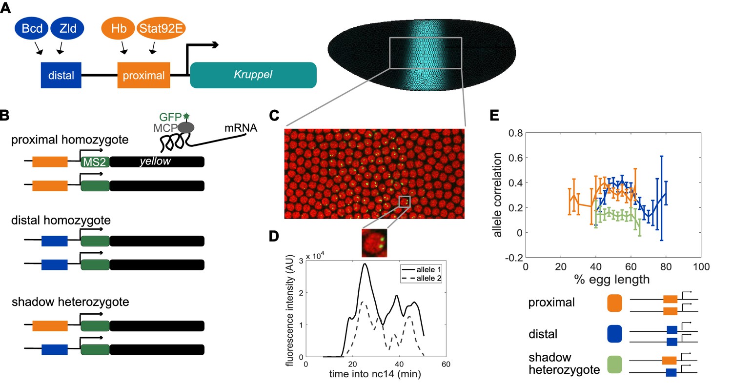
Dual allele imaging shows the individual Kruppel enhancers drive largely independent transcriptional dynamics.
(A) Schematic of the endogenous Kruppel locus with distal (blue) and proximal (orange) shadow enhancers driving Kr (teal) expression in the central region of the embryo. Known transcriptional activators of the two enhancers are shown. (B) Schematics of single enhancer reporter constructs driving expression of MS2 sequence and a yellow reporter. When transcribed, the MS2 sequence forms stem loops that are bound by GFP-tagged MCP expressed in the embryos. Proximal embryos have expression on each allele controlled by the 1.5 kb proximal enhancer at its endogenous spacing from the Kr promoter, while distal embryos have expression on each allele controlled by the 1.1 kb distal enhancer at the same spacing from the Kr promoter. Shadow heterozygote embryos have expression on one allele controlled by the proximal enhancer and expression on the other allele controlled by the distal enhancer. (C). Still frame from live imaging experiment where nuclei are red circles and active sites of transcription are green spots. MCP-GFP is visible as spots above background at sites of nascent transcription (Garcia et al., 2013). (D) The fluorescence of each allele in individual nuclei can be tracked across time as a measure of transcriptional activity. The graph shows a representative trace of transcriptional activity of the two alleles in a single nucleus across the time of nc14. These traces are used to calculate the Pearson correlation coefficient between the transcriptional activity of the two alleles in a nucleus across the time of nc14. Correlation values are grouped by position of the nucleus in the embryo and averaged across all imaged nuclei in all embryos of each construct. (E) Graph of average correlation between the two alleles in each nucleus as a function of egg length. 0% egg length corresponds to the anterior end. Error bars indicate 95% confidence intervals. The shadow heterozygotes have much lower allele correlation than either homozygote, demonstrating that the individual shadow enhancers drive nearly independent transcriptional activity and that upstream fluctuations in regulators are a significant driver of transcriptional bursts. The total number of nuclei used in calculations for each construct by anterior-posterior (AP) bin are given in Supplementary file 1.
Figure 1—figure supplement 1
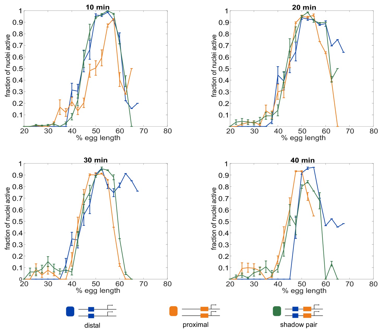
Fraction of nuclei transcribing as a function of embryo position.
The different enhancer constructs display different spatial and temporal patterns of activity. Shown in all graphs are the fraction of nuclei actively transcribing as a function of embryo position at each indicated time point into nc14. (A) 10 min into nc14. (B) 20 min into nc14. (C) 30 min into nc14. (D) 40 min into nc14. Error bars are 95% confidence intervals. We note that differences in the individual Kr enhancers become more pronounced throughout progression of nc14. The more anterior pattern driven by the proximal enhancer in the second half of nc14 mimics the anterior shift previously observed for the Kr expression domain (Jaeger et al., 2004; El-Sherif and Levine, 2016).
Figure 1—figure supplement 2
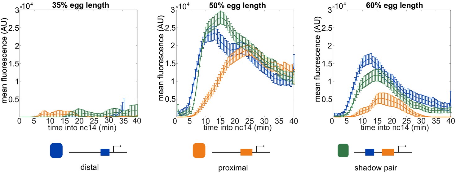
Expression across time at different embryo positions.
The activity levels of the different enhancer constructs vary both across time and space. Shown in each graph is the mean fluorescence of all transcriptional traces of the indicated enhancer construct as a function of time into nc14 at the indicated position in the embryo. The earlier activation of the shadow pair and distal enhancer compared to the proximal enhancer at 50% and 60% egg length may stem from the input of the pioneer TF Zelda (Zld) to the distal and shadow pair. Error bars are 95% confidence intervals.
Figure 1—figure supplement 3
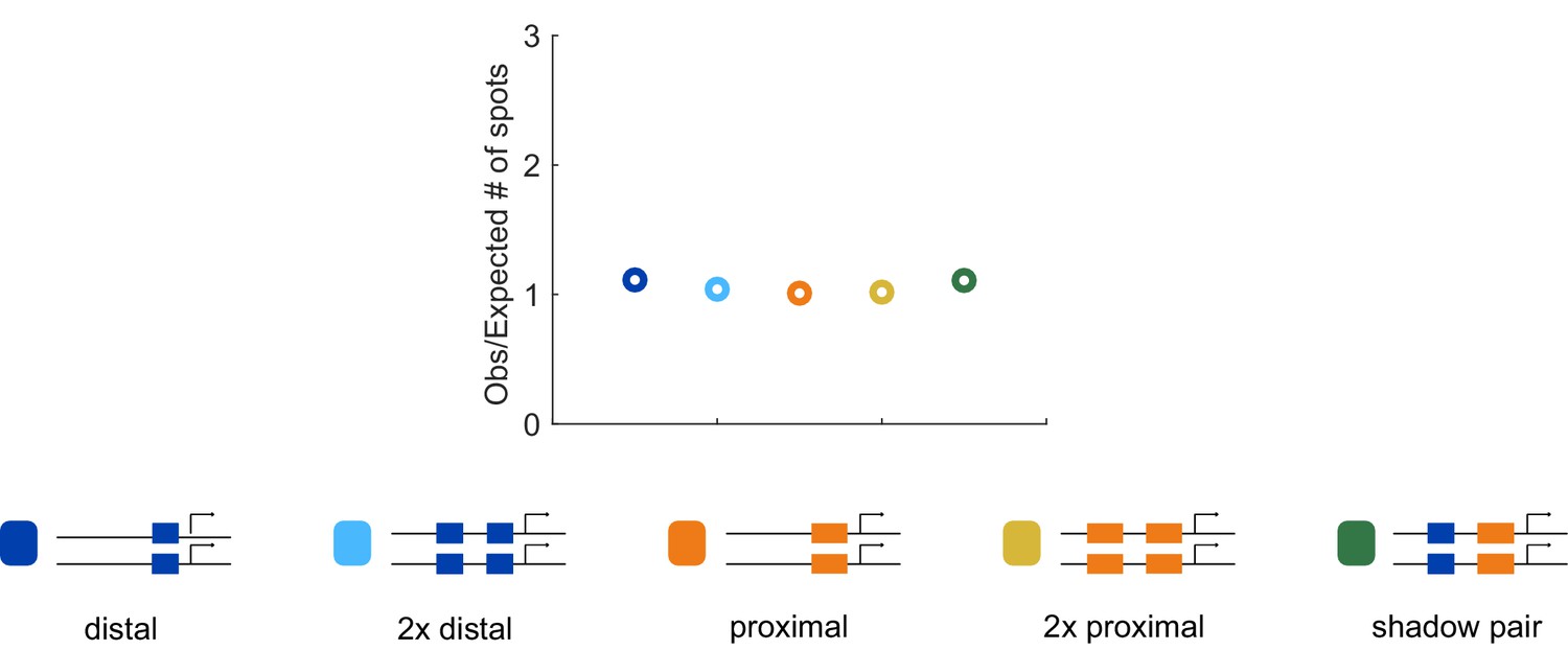
Correspondence of observed and expected number of spots.
To ensure that we can accurately measure two spots of expression in the embryo, we compared the number of transcriptional spots seen in embryos hemizygous or homozygous for each construct. Our rationale was that in the absence of transvection, the number of transcriptional spots in homozygous embryos should be twice the number in embryos expressing the reporter on only one allele. The number of transcriptional spots tracked during nc14 in the AP bin of maximum expression was counted for all embryos imaged for each homozygous and hemizygous construct. The graph shows the average of this value for homozygous embryos, divided by double the value observed in the corresponding hemizygous construct. Assuming no transvection occurs, this value should be close to 1. The ratio of observed to expected number of spots is close to one for all our enhancer constructs, indicating we are reliably able to track the two individual spots of transcription in single nuclei.
Figure 2 with 4 supplements
Model of enhancer-driven dynamics demonstrates TF fluctuations are required for correlated reporter activity.
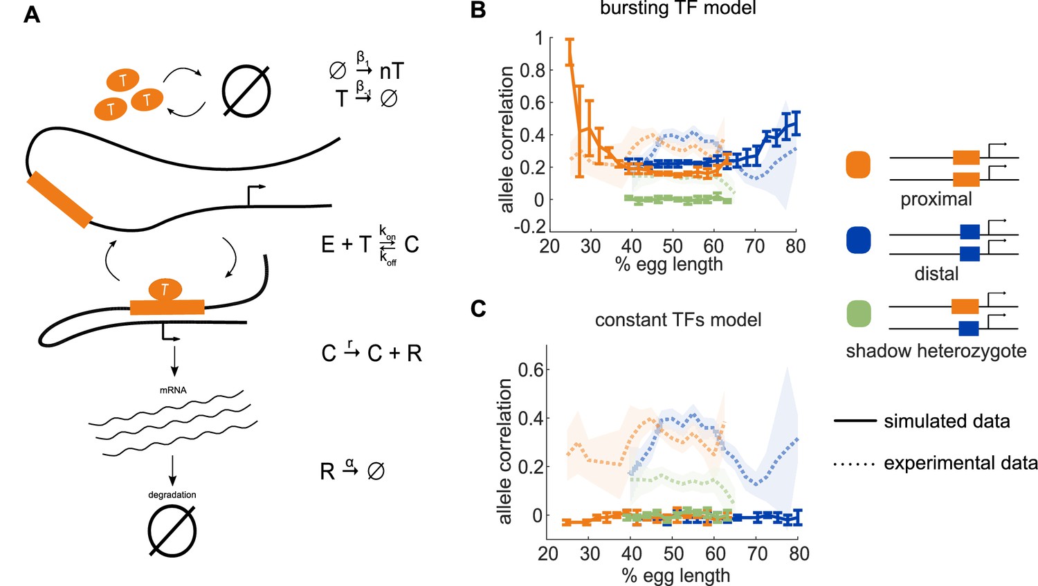
To investigate the factors required for the observed correlated behavior of identical enhancers and largely independent behavior of the individual enhancers, we developed a simple stochastic model of enhancer-driven transcription. (A) Schematic of model of transcription driven by a single enhancer (the bursting TFs model). For each enhancer, we assume there is a single activating TF, Ti, that appears in bursts of size ni molecules at a rate β1, which varies by the position in the embryo. TFs degrade linearly at rate β-1. When present, Ti can bind the enhancer, Ei, to form a transcriptionally active complex, Ci, at a rate kon and dissociates at rate koff. This complex then produces mRNA at an experimentally determined rate r that degrades at an experimentally determined rate, α. (B) The bursting TFs model is able to recapitulate the experimentally observed pattern of allele correlation. We plot the correlation between the two alleles in a nucleus as a function of egg length. Simulated data is created using the lowest energy parameter set for each enhancer. The data shown is the average of five simulated embryos that have 80 transcriptional spots per AP bin. In B and C, simulated data are shown by solid lines, experimental data are shown by dotted lines. (C) The constant TFs model fails to recapitulate the experimentally observed pattern of allele correlation. Without TF fluctuations, both heterozygous and homozygous embryos display independent allele activity. Error bars and shaded regions in B and C represent 95% confidence intervals.
Figure 2—figure supplement 1

Single enhancer models recreate observed transcriptional bursting properties.
To investigate whether our model is accurately simulating our experimental system, we compared the transcriptional burst properties produced by model simulations of transcription to those observed experimentally (see Figure 2—figure supplement 3 for description of burst properties). (A) Graphs of average values of transcriptional burst properties, total mRNA produced during nc14, burst frequency, burst duration, and burst size associated with the proximal enhancer as a function of egg length. In A and B, simulated data are represented with solid lines and experimental data are shown with dotted lines. (B) Graphs of average values of transcriptional burst properties as in A, associated with the distal enhancer. For both the proximal and distal enhancers, our model is largely able to recapitulate the experimentally observed transcriptional burst properties associated with each enhancer. (C) The median and CV values of the model parameters for the proximal enhancer in the top 10 performing parameter sets. (D) The median and CV values of the model parameters for the distal enhancer in the top 10 performing parameter sets. Explanations of model parameters are given in the Materials and methods. Error bars represent 95% confidence intervals.
Figure 2—figure supplement 2
Incorporating a common TF into the model yields nonzero heterozygote allele correlations.
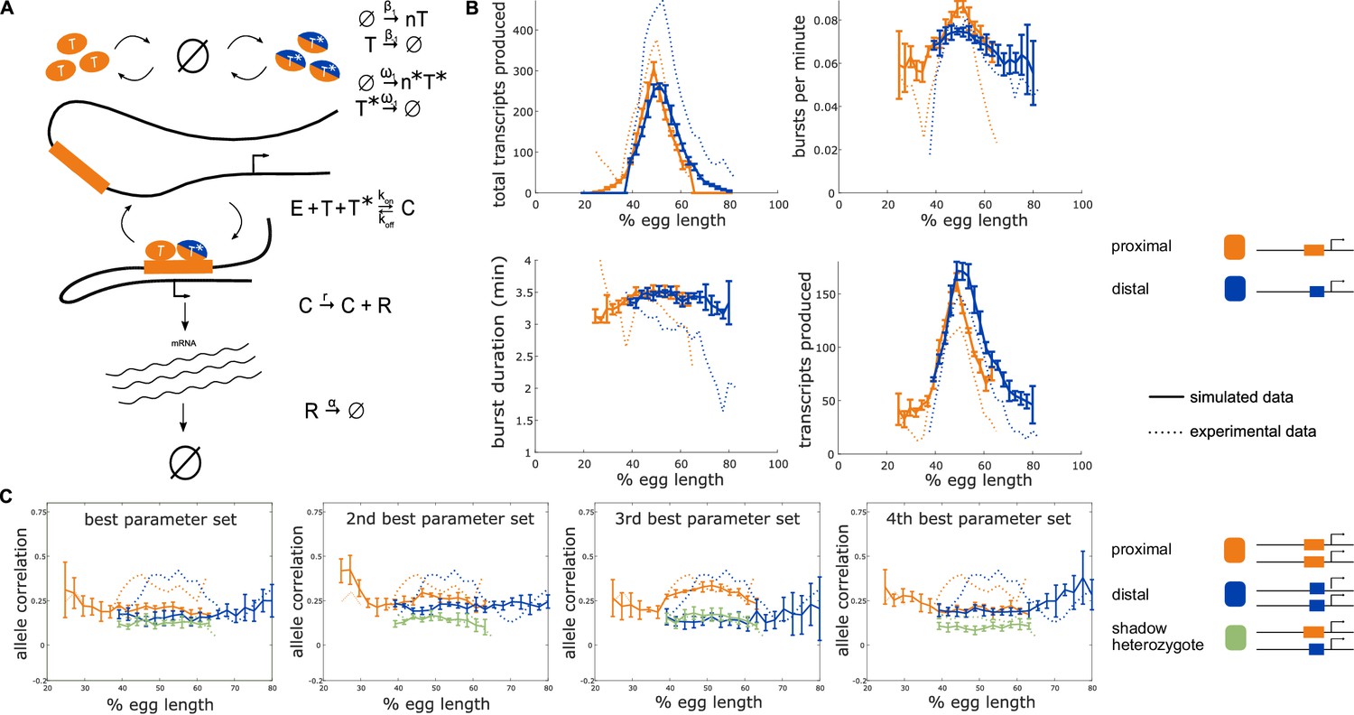
To determine whether the observed nonzero heterozygote correlation can be explained by common TF activity, we incorporated into our model a TF that can bind to both the proximal and distal enhancers. (A) Schematic of a model that includes an additional TF denoted T* which can bind to both the proximal and distal enhancers. The production of T* occurs at a rate ω1 which varies across the embryo in a similar manner to β1. T* degrades linearly at a rate ω-1 and appears in bursts of size n*. The presence of both the enhancer-specific TF Ti and the common TF T* are necessary to initiate transcription. (B) The addition of a common TF does not hinder the model from recapitulating the experimentally observed burst properties of single enhancer constructs. Simulated data is created using the second-best parameter set for each enhancer. The data shown is the average of five simulated embryos that have 80 transcriptional spots per AP bin. In B, C, and D simulated data are shown by solid lines, experimental data are shown by dotted lines. (C) The addition of the common TF T* consistently produces nonzero heterozygote allele correlations. However, some of the best parameter sets do not conserve the experimental relationship between homozygote and heterozygote correlations. Other parameter sets do not match the experimental data well, suggesting that the model accepts a narrower range of parameter combinations than the bursting TF model. Error bars in B and C represent 95% confidence intervals.
Figure 2—figure supplement 3
Visual inspection of burst calling algorithm.
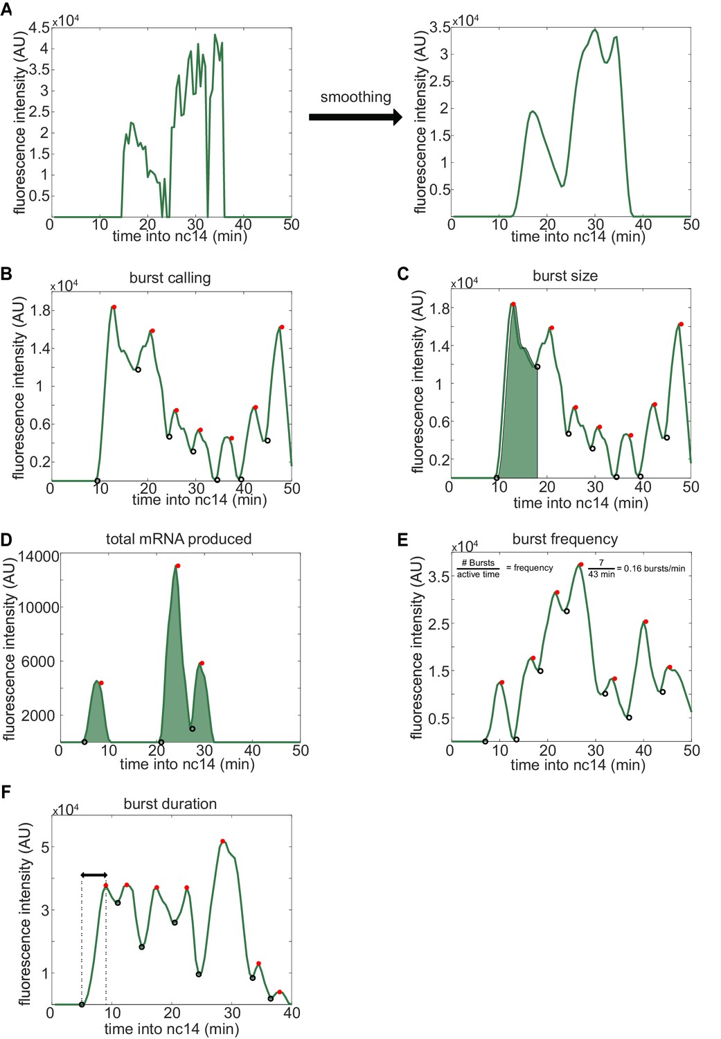
To extract the bursting parameters examined (burst size, frequency, and duration), individual fluorescence traces were first smoothed using the LOWESS method with a span of 0.1. Our burst calling algorithm then determined the periods of promoter activity or inactivity based on the slope of the fluorescence trace. (A) Representative example of smoothing of transcriptional traces. (B) Representative fluorescence trace of a single spot across the time of nc14. Black open circles indicate time points where the promoter is switched to being called ‘on’, red filled circles indicate time points where the promoter is switched to being called ‘off’. (C) A representative transcriptional trace with shading representing the area under the curve used to calculate the size of the first burst. This area is calculated using the trapz function in MATLAB and is done for each burst, from the time point the promoter is called ‘on’ until the next time it is called ‘on’. (D-F) show additional representative fluorescence traces of single transcriptional spots across the time of nc14. (D) A trace with shading representing the area under the entire curve during nc14 used to calculate the total amount of mRNA produced. This area is calculated using the trapz function in MATLAB and is done from the time the promoter is first called active until 50 min into nc14 or the movie ends, whichever comes first. (E) Burst frequency is calculated by dividing the number of bursts that occur from the time the promoter is first called active until 50 min into nc14 or the movie ends, whichever comes first. (F) Burst duration is defined as the amount of time between when the promoter is called active and it is next called inactive.
Figure 2—figure supplement 4

mRNA production and decay rates can be directly estimated from experimental data.
The mRNA degradation parameter α and production parameter r were measured directly from fluorescence data without any input from the model. (A) To estimate α, we used adjacent measurements of fluorescence intensity to approximate the slope at each point in the fluorescence traces. These values are compared with an exponential rate of mRNA decay (see Materials and methods) and the resulting predicted values are shown in the histogram. Periods of mRNA production have negative α values and periods of decay have positive values. The histogram shows a distinct peak for α > 0, which provided us with an estimate of α ≈ 1.95. (B) A similar computational approach was used to calculate values of r from fluorescence data (see Materials and methods). We calculated different values of r for each bin to account for differences in transcriptional efficiency across the length of the embryo due to factors that are not explicitly included in the model. For example, different combinations of TF bound to the enhancer may give rise to different mRNA production rates. Different values of r were found for the proximal and distal enhancers. Notice that distal r values shown correspond to the distal enhancer at the proximal location.
Figure 3
Activity of Kr shadow pair is less correlated with Bcd levels than is activity of single distal enhancer.
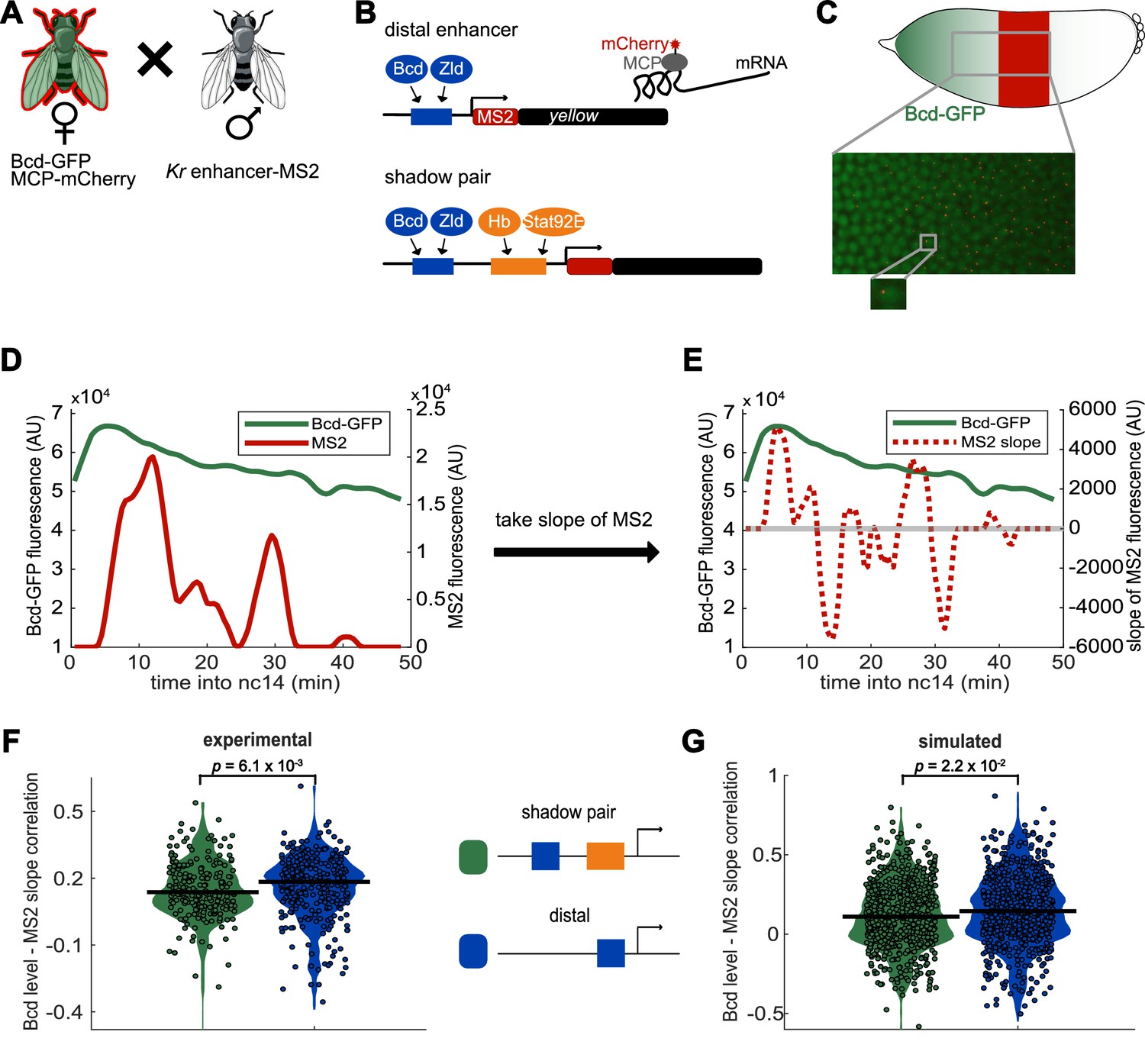
To assess whether fluctuations in enhancer activity across time are associated with fluctuations in TF levels, we simultaneously measured Bcd levels and enhancer-driven transcription in individual nuclei. (A) To track Bcd levels and enhancer activity in the same nuclei, we crossed flies expressing a Kr enhancer-MS2 transgene to flies expressing Bcd-GFP and MCP-mCherry. In the resulting embryos, Bcd levels can be measured by GFP fluorescence and enhancer reporter activity can be measured by mCherry fluorescence. (B) Schematic of the enhancer reporters used for simultaneous tracking of TF levels and enhancer activity. As in Figure 1, the transcribed MS2 sequence forms stem loops that are bound by MCP, which is here tagged with mCherry. (C) Bcd-GFP expression forms a gradient from the anterior to posterior of the embryo, whereas the Kr enhancer reporters drive expression in the center region of the embryo. The magnified section of the embryo shows a still frame from live imaging indicating nuclei (green) and active transcription spots (red). (D) Bcd levels and enhancer activity can be simultaneously tracked in individual nuclei. Graph shows a representative trace of Bcd-GFP levels (in green) and distal enhancer transcriptional activity (in red) in a nucleus across the time of nc14. (E) Activator TF levels regulate enhancer activity, so to assess the sensitivity of our enhancer constructs to input TF fluctuations, we compare the levels of nuclear Bcd-GFP to the slope of MS2 fluorescence across the time of nc14. Positive slope values indicate an increase in enhancer activity, while negative values indicate a decrease in enhancer activity. The graph shows nuclear Bcd-GFP levels (as in D), in solid green line, and MS2 slope values (of the MS2 trace shown in D), in dashed red line, across the time of nc14. Horizontal grey line indicates a slope value of 0. (F) Changes in the shadow pair’s activity are significantly less correlated with Bcd-GFP levels than are changes in the distal enhancer’s activity. Shown are violin plots of the distribution of correlation values between Bcd-GFP levels and MS2 slopes in individual nuclei for either the shadow pair or distal enhancer. Circles correspond to the correlation values of individual nuclei and the horizontal lines indicate the median. This correlation is significantly higher for the distal enhancer than it is for the shadow pair (median r values are 0.18 and 0.14, respectively. p-value=6.1×10⁻³ from Kruskal-Wallis pairwise comparison.) The total number of nuclei used in calculations for each construct by AP bin are given in Supplementary file 2. (G) Our enhancer model recapitulates the lower correlation between Bcd-GFP levels and enhancer activity seen with the shadow pair than with the distal enhancer. Graph is as in F, but showing the distribution of correlation values in simulated nuclei, using 100 nuclei per AP bin. Median r values for simulation are 0.14 for the distal enhancer and 0.11 for the shadow pair. p-value=2.2×10⁻² from Kruskal-Wallis pairwise comparison of correlations.
Figure 4 with 1 supplement
Shadow enhancer pair produces lower expression noise than duplicated enhancers.
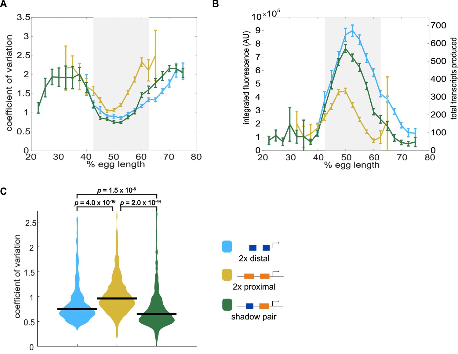
To investigate whether the shadow enhancer pair drives less noisy expression, we calculate the coefficient of variation (CV) associated with the shadow enhancer pair or either duplicated enhancer across time of nc14. (A) The shadow enhancer pair displays lower temporal expression noise than either duplicated enhancer. Graph is mean coefficient of variation of fluorescence traces across time as a function of embryo position. The grey rectangle in A and B highlights the region of endogenous Kr expression (boundaries where 33% maximal expression occurs). (B) The shadow enhancer pair shows the lowest expression noise, but not the highest expression levels, indicating that the lower noise is not simply a function of higher expression. Graph is average total expression during nc14 as a function of embryo position. Error bars in A and B represent 95% confidence intervals. Total number of transcriptional spots used for graphs are given in Supplementary file 3 by construct and AP bin. (C) Violin plot of distribution of CV values at AP bin of peak expression for each enhancer construct (corresponding to 50% egg length for shadow pair and duplicated proximal, 52.5% egg length for duplicated distal), horizontal bar indicates median. Y-axis limited to 99th percentile of the construct with highest expression noise (duplicated proximal). The shadow pair drives significantly lower expression noise than either duplicated enhancer (p-value=1.5×10⁻⁶ for duplicated distal and shadow pair. p-value=2.0×10−44 for duplicated proximal and shadow pair). p-Values were calculated using Kruskal Wallis pairwise comparison with Bonferroni multiple comparison correction.
Figure 4—figure supplement 1
Temporal CV as a function of mean fluorescence.
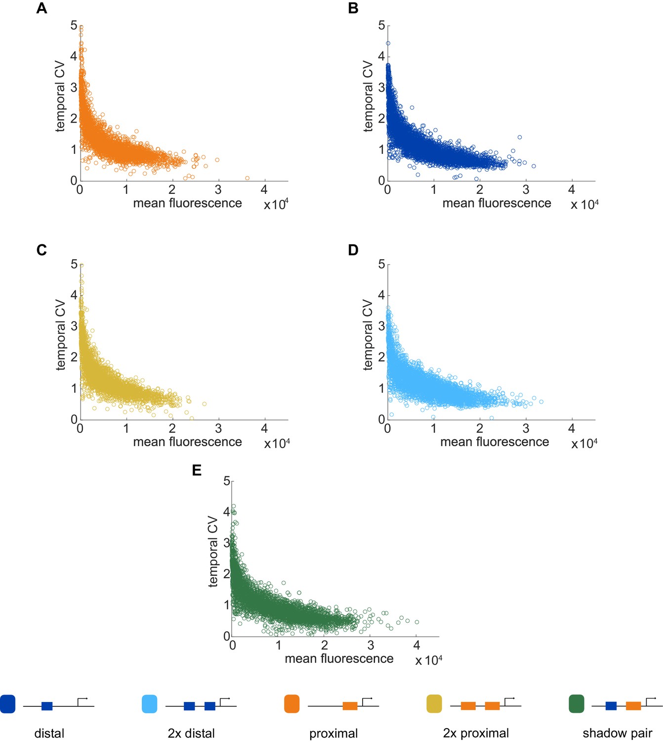
To investigate the relationship between our noise measurement of temporal CV and the mean activity of each construct, we plotted the temporal CV of each transcription spot as a function of its mean fluorescence. (A) Distal; (B) Proximal; (C) 2x Proximal; (D) 2x Distal; (E) Shadow pair. With all constructs, we find the general trend that CV decreases with increasing average expression, flattening out at a baseline noise level specific to each enhancer construct.
Figure 5 with 1 supplement
The two enhancer model recapitulates low expression noise associated with the shadow enhancer pair.
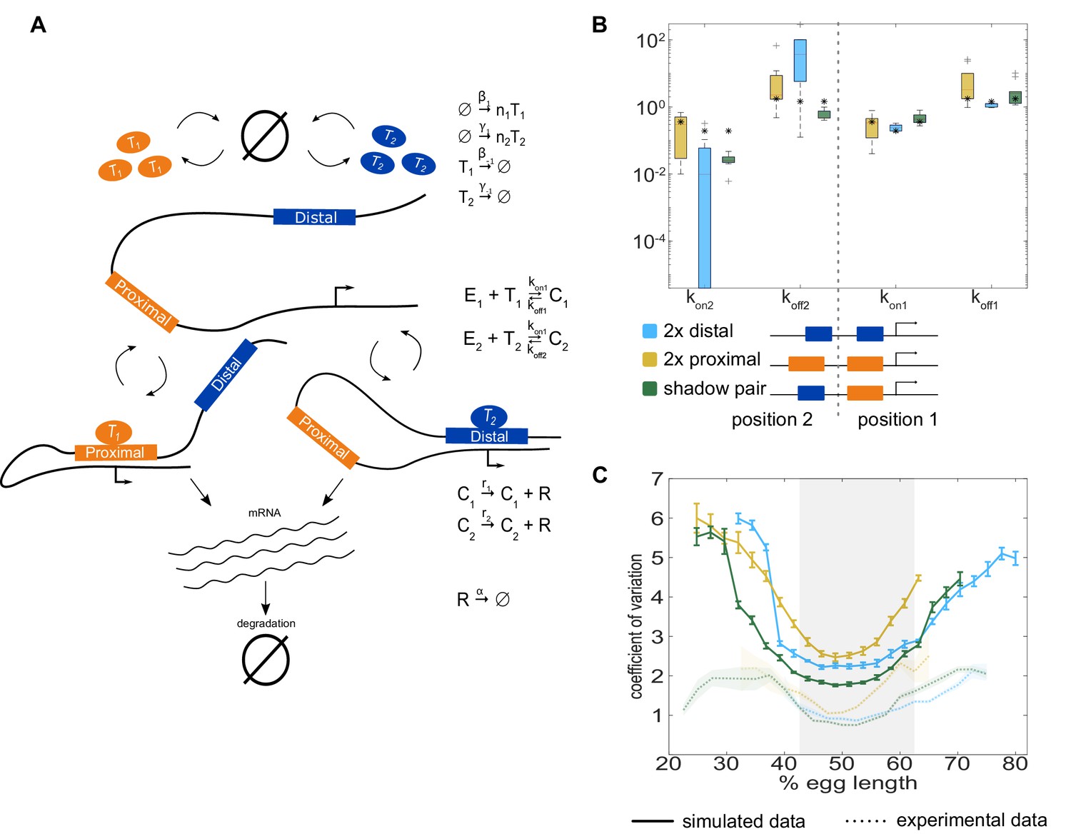
To assess whether the separation of input TFs mediates the lower expression noise driven by the shadow enhancer pair, we expanded our model to incorporate two enhancers driving transcription. (A) Schematic of the two enhancer model. We assume that when two enhancers control a single promoter, either or both can loop to the promoter and drive transcription. We defined model parameters as in Figure 2, and only allowed the kon and koff values to vary from the single enhancer model. (B) To understand the effect of adding a second enhancer, we examined how the kon and koff values vary from those in the single enhancer model. We plotted the distribution of the values for kon and koff for each enhancer in the three different constructs measured. The distribution shows the values derived from the 10 best-fitting parameter sets, and the black star in each column indicates the kon or koff value from the corresponding single enhancer model. In general, the koff values increased relative to the single enhancer model, and the kon values decreased, indicating that the presence of a second enhancer inhibits the activity of the first. (C) Graph of average coefficient of variation of simulated (solid lines) or experimental (dotted lines) transcriptional traces as a function of egg length. The model is able to recapitulate the lower expression noise seen with the shadow enhancer pair with no additional fitting, indicating that the separation of TF inputs to the two enhancers is sufficient to explain this observation. Error bars of simulated data and shaded region of experimental data indicate 95% confidence intervals.
Figure 5—figure supplement 1
Individual Kr enhancers display sub-additive behavior.
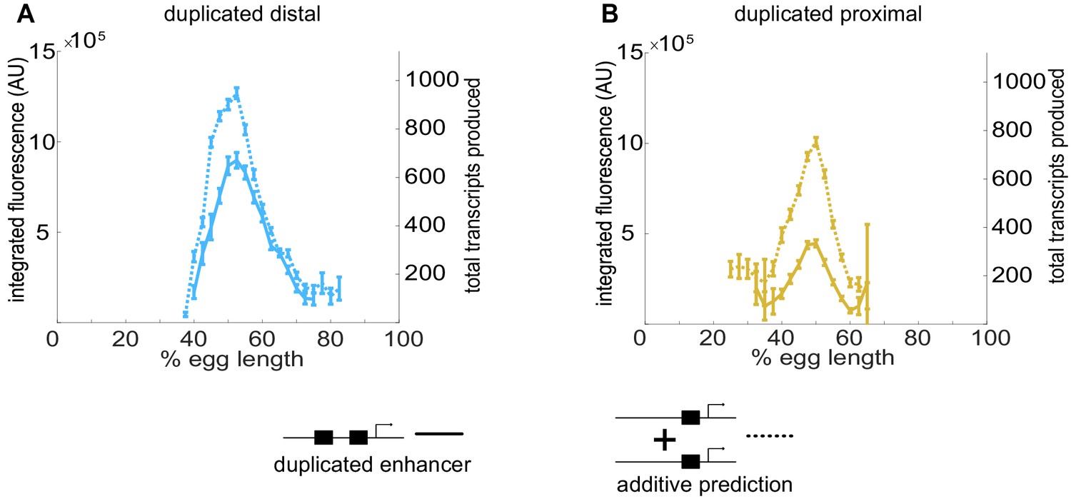
To assess the way input from two enhancers is integrated at the Kr promoter, we compared the experimentally observed mRNA production of duplicated enhancers to that predicted from additive behavior of the single enhancers. (A) The duplicated distal enhancer displays sub-additive behavior. The solid line is the experimentally observed total mRNA produced by the duplicated distal enhancer during nc14 as a function of egg length and the dotted line is that expected by doubling the total mRNA produced by the single distal enhancer. (B) The duplicated proximal enhancer also acts sub-additively. The solid line is the experimentally observed total mRNA produced by the proximal enhancer during nc14 as a function of egg length and the dotted line is that expected by doubling the total mRNA produced by the single proximal enhancer. These results, along with the observation that koff values increased and kon values decreased in our model with the addition of a second enhancer, suggests that the Kr enhancers compete with each other for interactions with the promoter. Error bars represent 95% confidence intervals.
Figure 6 with 3 supplements
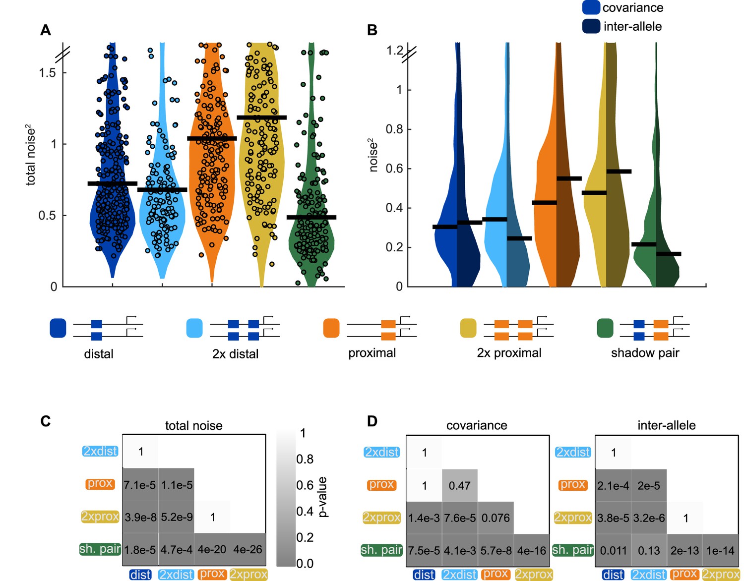
Shadow enhancer pair achieves lower total noise by buffering global and allele-specific sources of noise.
To determine how the shadow enhancer pair produces lower expression noise, we calculated the total noise associated with each enhancer construct and decomposed this into the contributions of covariance and inter-allele noise. Covariance is a measure of how the activities of the two alleles in a nucleus change together and is indicative of global sources of noise. Inter-allele noise is a measure of how the activities of the two alleles differ and is indicative of allele-specific sources of noise. (A) The shadow enhancer pair has lower total noise than single or duplicated enhancers. Circles are total noise values for individual nuclei in AP bin of peak expression for the given enhancer construct. Horizontal line represents the median. The y-axis is limited to 75th percentile of the proximal enhancer, which has the largest noise values. The shadow enhancer pair has significantly lower total noise than all other constructs. (B) The shadow enhancer pair displays significantly lower covariance than either single or duplicated enhancer and significantly lower inter-allele noise than both single enhancers and the duplicated proximal enhancer. The left half of each violin plot shows the distribution of covariance values of nuclei in the AP bin of peak expression, while the right half shows the distribution of inter-allele noise values. Horizontal lines represent median. The y-axis is again limited to the 75th percentile of enhancer with the largest noise values, which is duplicated proximal. The lower covariance and inter-allele noise associated with the shadow enhancer pair indicates it is better able to buffer both global and allele-specific sources of noise. (C) p-Value table of Kruskal-Wallis pairwise comparison of the total noise values of each enhancer construct. p-Value gradient legend applies to C and D. (D) p-Value table of Kruskal-Wallis pairwise comparison of covariance (on left) and inter-allele noise (on right) values for each enhancer construct. Bonferroni multiple comparison corrections were used for p-values in C and D. Total number of nuclei used in noise calculations are given in Supplementary file 1.
Figure 6—figure supplement 1

Fraction of nuclei with negative covariance of allele activity.
To identify the likely cause of the observed negative covariance between allele activity in some nuclei, we calculated the fraction of nuclei displaying negative covariance out of all nuclei that had active reporter transcription. Graphs show the fraction of transcribing nuclei with negative covariance as a function of egg length for each reporter construct, with a black circle indicating the position along the embryo of maximal expression for that construct. (A) Distal; (B) Proximal; (C) 2x Proximal; (D) 2x Distal; (E) Shadow pair. Note that for all constructs, the highest rates of negative covariance are outside of the region of maximal reporter expression. MCP-GFP is expressed uniformly along the length of the embryo and we would therefore expect if MCP-GFP were the limiting factor, we would see the highest rates of negative covariance in the center of the expression pattern, where the highest number of transcripts are produced. Instead, the highest rates of negative covariance are seen at the edges of the Kr expression pattern, suggesting a spatially patterned factor, such as a TF, may be what is limiting.
Figure 6—figure supplement 2
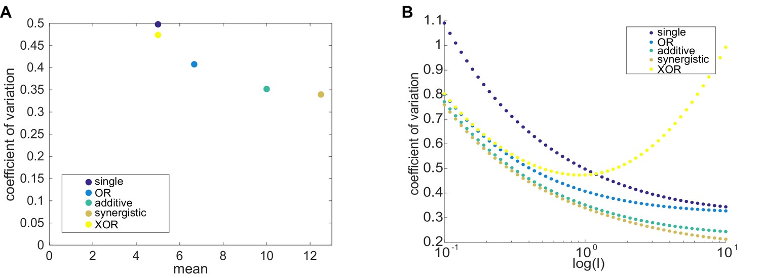
In most cases, two enhancer models drive lower noise than the single enhancer model.
To theoretically explore the behavior of instrinsic noise in one- and two-enhancer models, we used the formalism of Sanchez et al., 2011; Sánchez and Kondev, 2008. As described in Materials and methods, the predicted CVs from these models are estimates for intrinsic noise. (A) We plot the mean expression level versus CV for the five different enhancer models and one set of parameters, k = l = 1, p=1, γ = 0.1. The single enhancer model (dark purple) drives the highest CV, indicating that, under the assumptions of our models, adding an additional enhancer generally lowers intrinsic noise. Except for XOR model (yellow), all other models produce more mRNA than the single enhancer model. The other colors are: blue, OR model; green, additive model; brown, synergistic model. (B) Here, we plot the CV as a function of l, the rate of promoter-enhancer dissociation, for the five models above and vary l from 0.1 to 10 on a logarithmic scale with k = 1, p=1, γ = 0.1. With the exception of the XOR model with high l, the single enhancer model drives a higher CV than the models with two enhancers for the same value of l. These results show that, under the simplifying assumptions made in these models, the addition of a second enhancer generally lowers the predicted intrinsic noise. In our experimental data (Figure 6), we only observe a significant decrease in interallele noise for the shadow enhancer pair compared to the single distal or single proximal enhancer. Duplications of either the proximal or distal enhancer do not have significantly lower noise than their respective single enhancer constructs. Therefore, we expect that the simple addition of an identical enhancer likely does not fulfill the simplifying parameter assumptions used here and suggests that further investigation is needed to understand the complexity of the relationship between interallele noise and the numbers of enhancers controlling a promoter.
Figure 6—figure supplement 3
Position-dependent effects on distal enhancer.
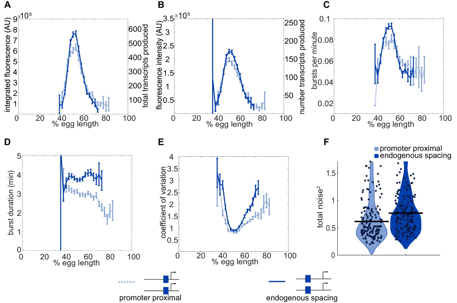
To best mimic the endogenous system, we looked at expression driven by the distal enhancer at its endogenous spacing from the promoter for our noise calculations. In this construct, we replaced the sequence of the proximal enhancer with sequence of the same length from the lambda phage genome predicted to have low number of Drosophila TF binding sites. This increased distance from the promoter had observable effects on the transcriptional dynamics and noise associated with the distal enhancer. (A) Comparison of total transcriptional expression mediated by the distal enhancer at its endogenous spacing or proximal to the promoter. The distal enhancer at its endogenous spacing, shown as the solid line, produces significantly more total mRNA in the center region of expression than the distal enhancer proximal to the promoter, shown as the dotted line. (B) Comparison of the average number of transcripts produced per transcriptional burst by each distal enhancer configuration as a function of egg length. (C) Average burst frequency associated with either distal enhancer configuration as a function of egg length. (D) Average burst duration associated with either distal enhancer configuration as a function of egg length. (E) Coefficient of variation of transcriptional activity across nc14 for each distal enhancer configuration as a function of egg length. (F) Total expression noise associated with either distal enhancer configuration at the AP bin of that construct’s peak expression. The total noise distribution for the distal enhancer proximal to the promoter is on the left and that for the distal enhancer at its endogenous spacing from the promoter is on the right. The distal enhancer at its endogenous spacing displays significantly higher total noise (p=0.018) than the distal enhancer proximal to the promoter. Each circle represents the total noise of an individual nucleus and the horizontal bar marks the median total noise value. Y-axis limited to the 75th percentile of the construct with the highest total noise values (distal promoter at endogenous spacing). Error bars in A-E represent 95% confidence intervals.
Figure 7
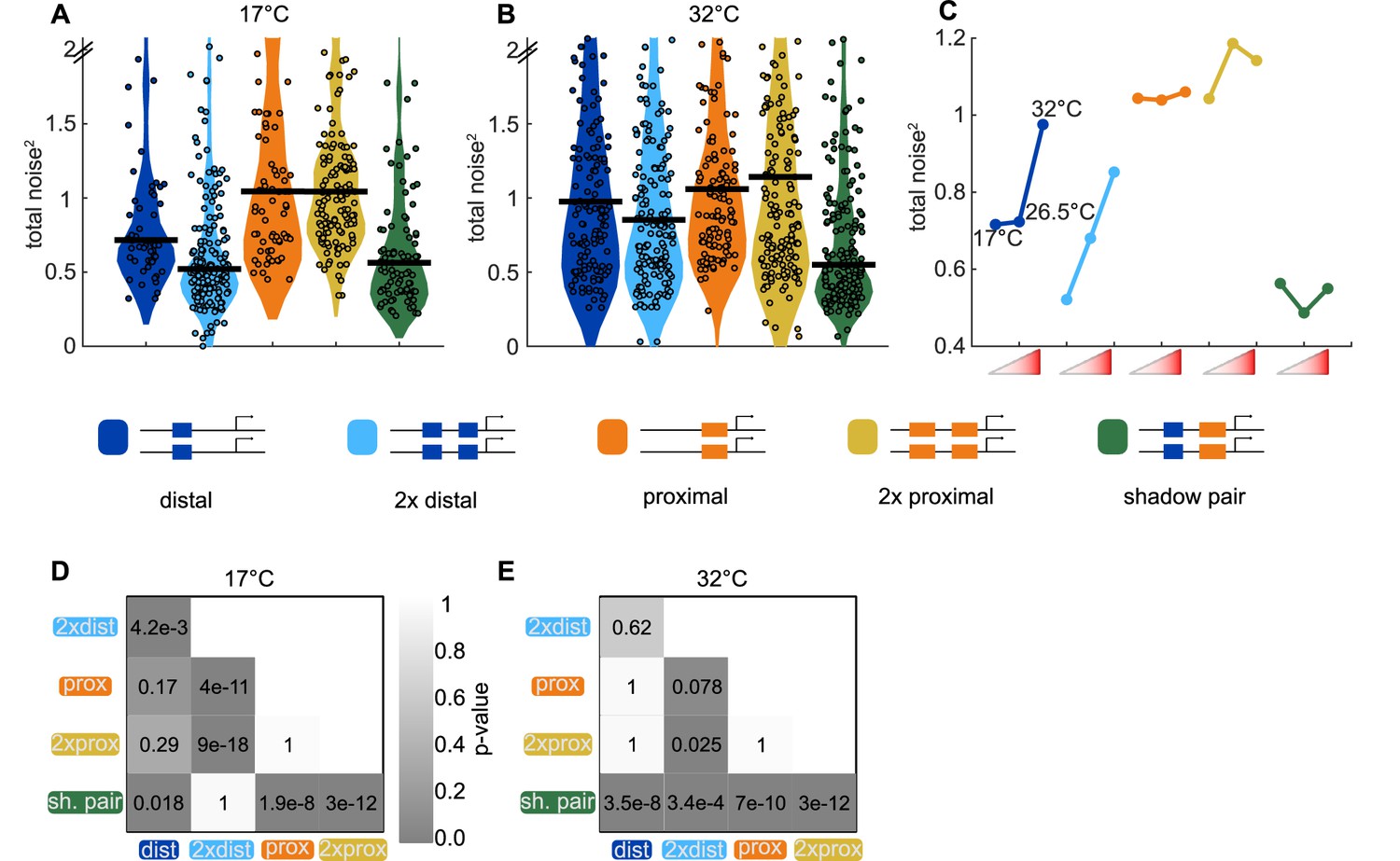
Shadow enhancer pair maintains lower total noise across temperature perturbations.
To test the ability of each enhancer construct to buffer temperature perturbations, we measured the total expression noise associated with each for embryos imaged at 17°C or 32°C. (A) The shadow enhancer pair displays significantly lower total noise than the single or duplicated proximal enhancer and the single distal enhancer at 17°C. Circles are total noise values for individual nuclei in AP bin of peak expression for the given enhancer construct and horizontal bars represent medians. The y-axis is limited to 75th percentile of construct with highest total noise at 17°C (single proximal). (B) The shadow enhancer pair has significantly lower total noise than all other constructs at 32°C. The y-axis is limited to 75th percentile of the enhancer construct with highest total noise at 32°C (duplicated proximal). (C) Temperature changes have different effects on the total noise associated with the different enhancers. The median total noise value at the AP bin of peak expression at the three measured temperatures is shown for each enhancer construct. Within each enhancer, the median total noise values are shown left to right for 17°C, 26.5°C, and 32°C. (D) p-Value table of Kruskal-Wallis pairwise comparison of the total noise values of each enhancer construct at 17°C. p-value gradient legend applies to D and E. (E) p-Value table of Kruskal-Wallis pairwise comparison of the total noise values of each enhancer construct at 32°C. Bonferroni multiple comparison corrections were used for p-values in D and E.
Videos
Video 1
Transcriptional dynamics of distal enhancer reporter homozygotes.
Movie showing maximum projection of transcription driven by the distal enhancer reporter in homozygous embryos from 15 min into nc14 through 35 min into nc14. Anterior is to the left and dorsal side is up. Elapsed time of movie is shown in upper right corner. Imaging region is centered at approximately 37% egg length.
Video 2
Transcriptional dynamics of proximal enhancer reporter homozygotes.
Movie showing maximum projection of transcription driven by the proximal enhancer reporter in homozygous embryos in the end of nc12 through the first 16 min of nc14. Anterior is to the left and dorsal side is up. Elapsed time of movie is shown in upper right corner. Imaging region is centered at approximately 50% egg length.
Video 3
Transcriptional dynamics of shadow heterozygote embryos.
Movie showing maximum projection of transcription driven by the shadow heterozygote embryos from end of nc13 through the first 15 min of nc14. Anterior is to the left and dorsal side is up. Elapsed time of movie is shown in upper right corner. Imaging region is centered at approximately 55% egg length.
Video 4
Transcriptional dynamics of duplicated distal reporter homozygotes.
Movie showing maximum projection of transcription driven by the duplicated distal reporter in homozygous embryos in the second half of nc13 through the first 15 min of nc14. Anterior is to the left and dorsal side is up. Elapsed time of movie is shown in upper right corner. Imaging region is centered at approximately 55% egg length.
Video 5
Transcriptional dynamics of duplicated proximal reporter homozygotes.
Movie showing maximum projection of transcription driven by the duplicated proximal reporter in homozygous embryos from 15 min into nc14 to 30 min into nc14. Anterior is to the left and dorsal side is up. Elapsed time of movie is shown in upper right corner. Imaging region is centered at approximately 50% egg length.
Video 6
Transcriptional dynamics of shadow enhancer pair homozygotes.
Movie showing maximum projection of transcription driven by the shadow pair reporter in homozygous embryos at the end of nc13 through the first 15 min of nc14. Anterior is to the left and dorsal side is up. Elapsed time of movie is shown in upper right corner. Imaging region is centered at approximately 50% egg length.
Video 7
Simultaneous tracking of Bcd-GFP and distal enhancer activity.
Movie showing maximum projection of Bcd-GFP (green) and transcription driven by the distal enhancer reporter (red) in the first 15 min of nc14. Anterior is to the left and dorsal side is up. Elapsed time of movie is shown in upper right corner. Imaging region is centered at approximately 37% egg length. Contrast increased by 0.3% for improved visibility.
Video 8
Simultaneous tracking of Bcd-GFP and shadow pair activity.
Movie showing maximum projection of Bcd-GFP (green) and transcription driven by the shadow pair reporter (red) at the end of nc13 through 40 min into nc14. Anterior is to the left and dorsal side is up. Elapsed time of movie is shown in upper right corner. Imaging region is centered at approximately 37% egg length. Contrast increased by 0.3% for improved visibility.
Tables
Key resources table
| Reagent type (species) or resource | Designation | Source or reference | Identifiers | Additional information |
|---|---|---|---|---|
| Genetic reagent (Drosophila melanogaster) | ChrII attP site; PBac{y[+]-attP-3B}VK00002 | Bloomington Drosophila Stock Center | BDSC:9723 FLYB: FBti0076425 | Fly line injected for transgenic reporters |
| Genetic reagent (D. melanogaster) | Kr proximal enhancer | This paper | Fly line with MS2 expression driven by Kr proximal enhancer inserted on chromosome II | |
| Genetic reagent (D. melanogaster) | Kr distal enhancer | This paper | Fly line with MS2 expression driven by Kr distal enhancer inserted on chromosome II | |
| Genetic reagent (D. melanogaster) | shadow enhancer pair | This paper | Fly line with MS2 expression driven by Kr shadow enhancer pair inserted on chromosome II | |
| Genetic reagent (D. melanogaster) | duplicated distal enhancer | This paper | Fly line with MS2 expression driven by two copies of Kr distal enhancer inserted on chromosome II | |
| Genetic reagent (D. melanogaster) | duplicated proximal enhancer | This paper | Fly line with MS2 expression driven by two copies of Kr proximal enhancer inserted on chromosome II | |
| Genetic reagent (D. melanogaster) | endogenous distal enhancer | This paper | Fly line with MS2 expression driven by Kr distal enhancer at endogenous spacing from promoter, inserted on chromosome II | |
| Genetic reagent (D. melanogaster) | Bcd-GFP; Bcd-eGFP | Gregor et al., 2007, Cell | Fly line with mutated endogenous Bcd (bcdE1) rescued with GFP-tagged Bcd transgene on X chromosome | |
| Genetic reagent (D. melanogaster) | MCP-GFP | Garcia et al., 2013, Current Biology | Fly line expressing MCP-GFP on chromosome III and His-RFP on chromosome II | |
| Genetic reagent (D. melanogaster) | MCP-mCherry | Hernan Garcia Lab | Fly line expressing MCP-mCherry as transgene on Chromosome II | |
| Genetic reagent (D. melanogaster) | hunchback P2 enhancer | Garcia et al., 2013, Current Biology | Fly line with MS2 expression driven by hb P2 enhancer on chromosome II | |
| Software, algorithm | mRNADynamics | Garcia et al., 2013, Current Biology | MATLAB pipeline for tracking and analysing MS2 transcriptional spots |
Additional files
-
Supplementary file 1
Number of nuclei tracked for each construct.
Each row corresponds to a construct, named in column 42, and columns 1–41 correspond to that AP bin of the embryo. The value in each cell in columns 1–41 is the number of nuclei used for correlation and total noise/covariance/inter-allele noise calculations in that AP bin for the given construct. The value in column 43 is the total number of independently imaged embryos for that construct.
- https://cdn.elifesciences.org/articles/59351/elife-59351-supp1-v2.xls
-
Supplementary file 2
Number of nuclei tracked for TF levels - enhancer activity comparisons.
Each row corresponds to a construct, named in column 42, and columns 1–41 correspond to that AP bin of the embryo. The value in each cell in columns 1–41 is the number of nuclei used for Bcd-GFP - MS2 slope correlation calculations in that AP bin for the indicated construct. The value in column 43 is the total number of independently imaged embryos for that construct.
- https://cdn.elifesciences.org/articles/59351/elife-59351-supp2-v2.xls
-
Supplementary file 3
Number of total single alleles tracked for each construct.
Each row corresponds to a construct, named in column 42, and columns 1–41 correspond to that AP bin of the embryo. The value in each cell in columns 1–41 is the number of single transcriptional spots used in calculations of burst size, frequency, and duration and CV in that AP bin for the given construct. The value in column 43 is the total number of independently imaged embryos for that construct.
- https://cdn.elifesciences.org/articles/59351/elife-59351-supp3-v2.xls
-
Supplementary file 4
The sequences of all the enhancer constructs generated in this paper.
- https://cdn.elifesciences.org/articles/59351/elife-59351-supp4-v2.txt
-
Transparent reporting form
- https://cdn.elifesciences.org/articles/59351/elife-59351-transrepform-v2.docx
Download links
A two-part list of links to download the article, or parts of the article, in various formats.
Downloads (link to download the article as PDF)
Open citations (links to open the citations from this article in various online reference manager services)
Cite this article (links to download the citations from this article in formats compatible with various reference manager tools)
Shadow enhancers can suppress input transcription factor noise through distinct regulatory logic
eLife 9:e59351.
https://doi.org/10.7554/eLife.59351


