Do wealth and inequality associate with health in a small-scale subsistence society?
- Institute of Evolutionary Medicine, University of Zurich, Switzerland
- Department of Anthropology, Emory University, United States
- Department of Anthropology, Washington State University, United States
- Jepson School of Leadership Studies, University of Richmond, United States
- School of Human Evolution and Social Change, Arizona State University, United States
- Center for Evolution and Medicine, School of Life Sciences, Arizona State University, United States
- Institute for Advanced Study in Toulouse, France
- Department of Anthropology, University of California, Santa Barbara, United States
- Department of Human Behavior, Ecology and Culture, Max Planck Institute for Evolutionary Anthropology, Germany
- Economic Science Institute, Chapman University, United States
- Department of Anthropology, University of New Mexico, United States
Figures
Figure 1 with 1 supplement

Overview of wealth and inequality distributions.
(A) Mean wealth by age of household head. (B) Mean wealth by population-level wealth Z-score. (C) Map of study communities (n = 40) and mean wealth at the community level. (D) Map of community-level wealth inequality. Note: (A) and (B) use raw wealth, while (C) and (D) are based on age-corrected values. Heat maps in (C) and (D) give a rough sense of the distribution; circle size indicates the number of sampled households (range = 9–81). Data for individual villages are not directly shown to protect confidentiality. Yucumo and San Borja are local market towns inhabited by non-Tsimane, Mission is the site of a Catholic mission and the largest Tsimane settlement.
Figure 1—figure supplement 1
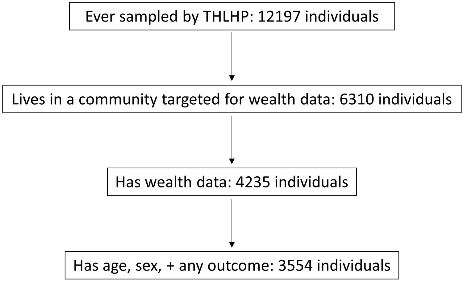
Overview of the sample.
Ever sampled by THLHP refers to the period potentially included in this study, that is, up to December 2015; note that this sample includes 92 communities. Target communities (N = 40) were those with any wealth data collected during the periods included here (2006/2007, 2013). The main reason why 2075 people who lived in a target community did not have wealth data is likely that no one in their household was available to be interviewed about their assets, most likely because they were temporarily absent from the community (e.g., people sometimes stay near their far-away fields, go on extended hunting trips, or visit town or other communities). The majority of the 681 individuals who lived in a household with wealth data but lacked age, sex, and data on at least one of the outcome variables were most likely small children and infants who had not yet been sampled in detail. For a further missingness breakdown of the sample by specific outcome variable, see Table 1. THLHP: Tsimane Health and Life History Project.
Figure 2 with 3 supplements
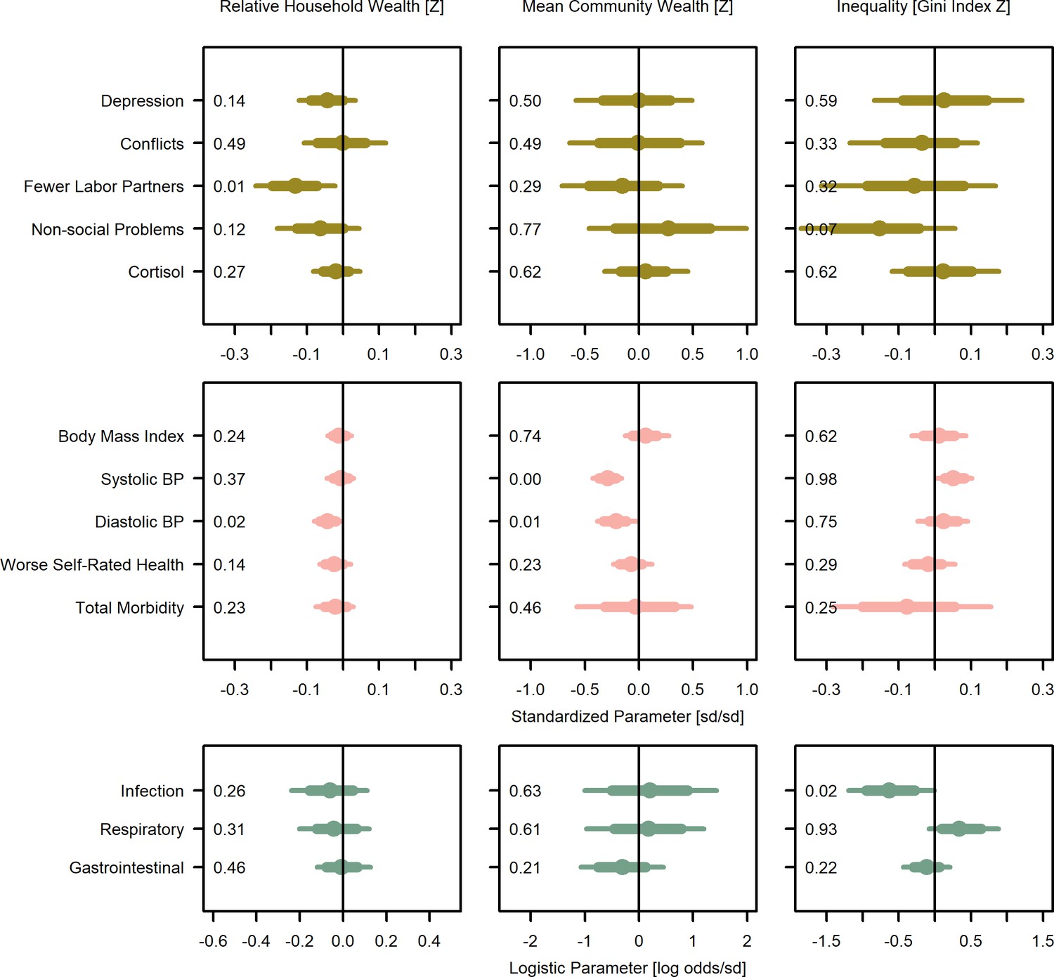
Wealth and inequality posterior parameter values for models with adults (>15 years).
Points are posterior medians and lines are 75% (thick) and 95% (thin) highest posterior density intervals. Numbers in each panel represent the proportion of the posterior distribution that is greater than zero (P>0). All models control for age, sex, distance to market town, and community size. Rough categories of dependent variables (psychosocial, continuous health outcomes, and binary health outcomes) are distinguished by rows and colors. For the first two rows, the outcomes are expressed as Z-scores, the bottom row as log odds. See Figure 2—figure supplement 1, Figure 2—figure supplement 2, and Figure 2—figure supplement 3 for predicted associations of household wealth, community wealth, and wealth inequality, respectively.
Figure 2—figure supplement 1
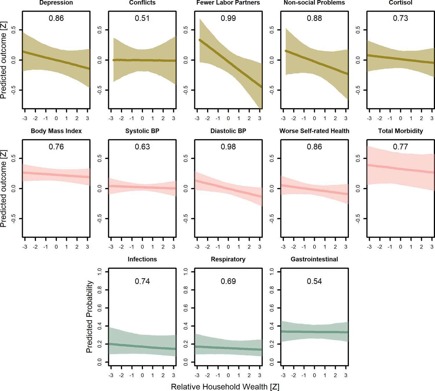
Predicted conditional effects of relative household wealth on all psychosocial and health outcomes for adults.
Lines are posterior means and shaded areas are 95% credible intervals on mean values. Numbers in each panel represent the proportion of the posterior distribution that supports the predicted negative association between wealth and the outcome (P<0). All predictions control for age, sex, inequality, distance to market town, community size, and mean community wealth, holding all other variables at the mean, with sex = female. Rough categories of dependent variables (psychosocial, continuous health outcomes, and binary health outcomes) are distinguished by rows and colors. For the first two rows, the outcomes are measured as Z-scores, the bottom row as probabilities.
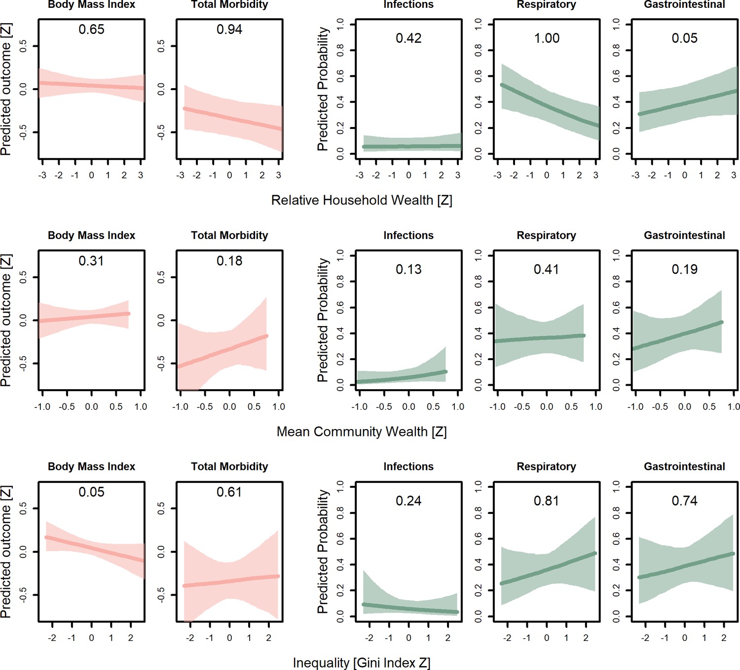
Figure 2—figure supplement 2
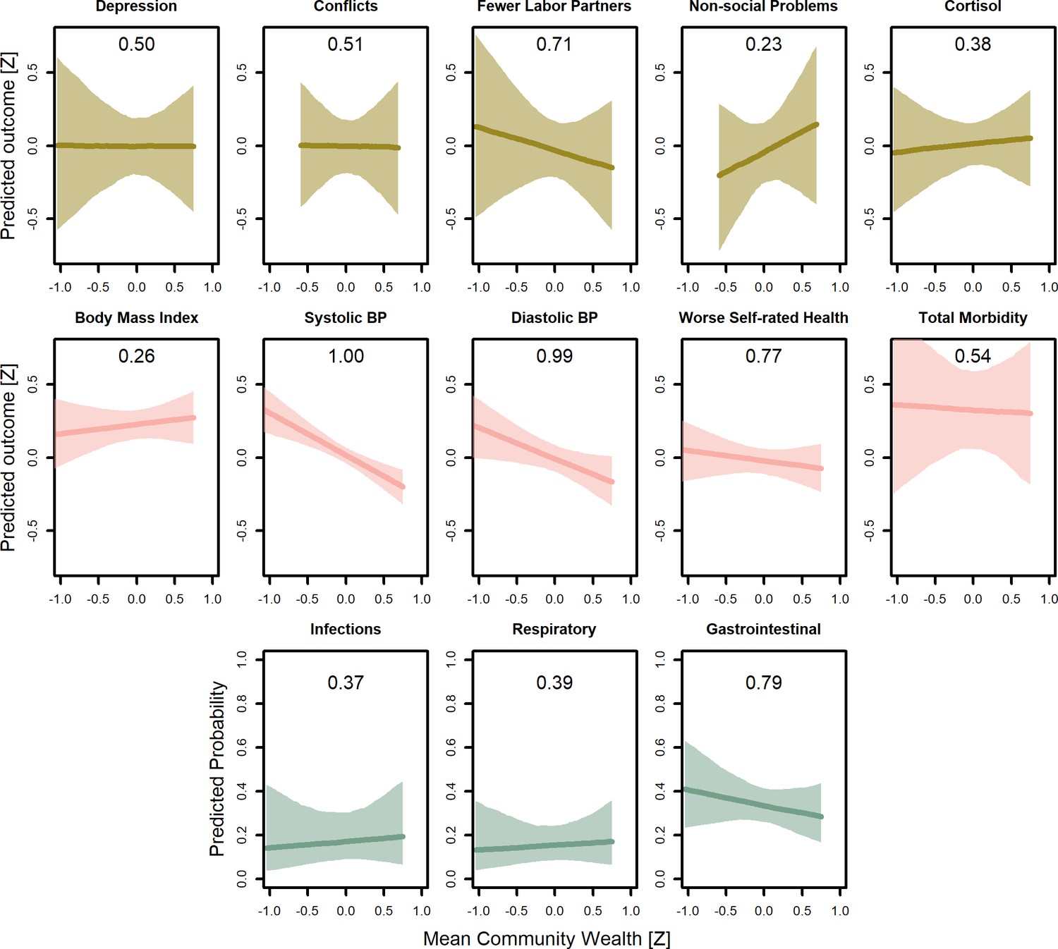
Predicted conditional effects of mean community wealth on all psychosocial and health outcomes for adults.
Lines are posterior means and shaded areas are 95% credible intervals on mean values. Numbers in each panel represent the proportion of the posterior distribution that supports the predicted negative association between wealth and the outcome (P<0). All predictions control for age, sex, inequality, distance to market town, community size, and mean community wealth, holding all other variables at the mean, with sex = female. Rough categories of dependent variables (psychosocial, continuous health outcomes, and binary health outcomes) are distinguished by rows and colors. For the first two rows, the outcomes are measured as Z-scores, the bottom row as probabilities.
Figure 2—figure supplement 3
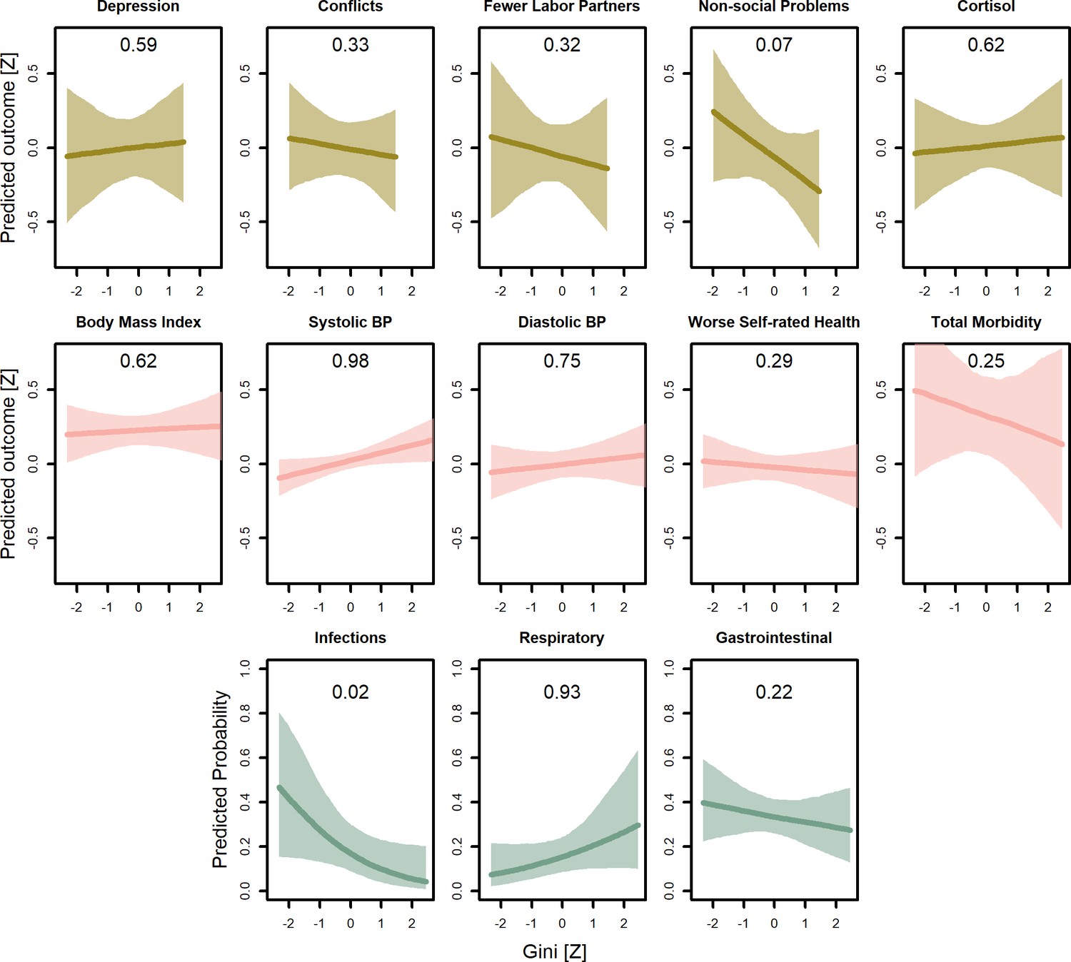
Predicted conditional effects of wealth inequality (Gini coefficients) on all psychosocial and health outcomes for adults.
Lines are posterior means and shaded areas are 95% credible intervals on mean values. Numbers in each panel represent the proportion of the posterior distribution that supports the predicted negative association between wealth and the outcome (P<0). All predictions control for age, sex, inequality, distance to market town, community size, and mean community wealth, holding all other variables at the mean, with sex = female. Rough categories of dependent variables (psychosocial, continuous health outcomes, and binary health outcomes) are distinguished by rows and colors. For the first two rows, the outcomes are measured as Z-scores, the bottom row as probabilities.
Figure 3 with 1 supplement

Wealth and inequality posterior parameter values for models with juveniles (≤15 years).
Points are posterior medians and lines are 75% (thick) and 95% (thin) highest posterior density intervals. Numbers in each panel represent the proportion of the posterior distribution that is greater than zero (P>0). All models control for age, sex, distance to market town, and community size. Rough categories of dependent variables (continuous health outcomes and binary health outcomes) are distinguished by rows and colors. For the first row, the outcomes are measured as Z-scores, the bottom row as log odds. See Figure 3—figure supplement 1 for predicted associations of household wealth, community wealth, and wealth inequality.
Figure 3—figure supplement 1
Predicted conditional effects of household wealth, community wealth, and inequality (Gini coefficients) on all health outcomes for juveniles (<15 years).
Lines are posterior means and shaded areas are 95% credible intervals on mean values. Numbers in each panel represent the posterior probability, that is, the proportion of the posterior that supports an association between inequality and the outcome. All predictions control for age, sex, distance to market town, and community size, holding all other variables at the mean, with sex = female. For the first two columns, the outcomes are measured as Z-scores, the remainder as probabilities.
Figure 4

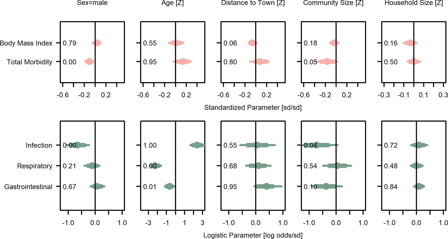
Covariate posterior parameter values for models with adults (>15 years).
Points are posterior medians and lines are 75% (thick) and 95% (thin) highest posterior density intervals. Numbers in each panel represent the proportion of the posterior distribution that is greater than zero (P>0). Full models are given in Supplementary file 1a-1m. Rough categories of dependent variables (psychosocial, continuous health outcomes, and binary health outcomes) are distinguished by rows and colors. For the first two rows, the outcomes are measured as Z-scores, the bottom row as log odds.
Figure 5
Covariate posterior parameter values for models with juveniles (≤15 years).
Points are posterior medians and lines are 75% (thick) and 95% (thin) highest posterior density intervals. Numbers in each panel represent the proportion of the posterior distribution that is greater than zero (P>0). Full models are given in Supplementary file 1n and o. Rough categories of dependent variables (continuous health outcomes and binary health outcomes) are distinguished by rows and colors. For the first row, the outcomes are measured as Z-scores, the bottom row as log odds.
Figure 6
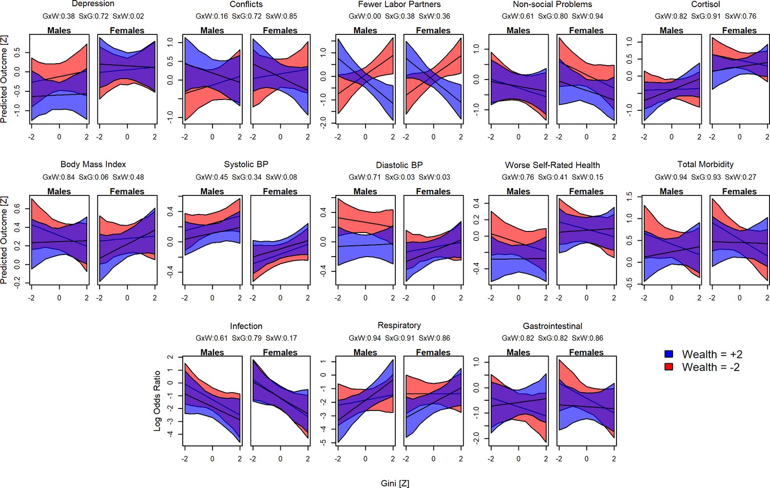
Interactions between sex, wealth, and inequality.
Plots show the predicted values for each outcome and Gini Z-score. Red shading indicates poorer individuals (wealth Z = –2), blue indicates wealthier individuals (Z = 2). For each model, the proportion of the posterior >0 is shown in the numbers above: GxW: Gini × Wealth; SxG = Sex × Gini; SxW = Sex × Wealth.
Appendix 1—figure 1
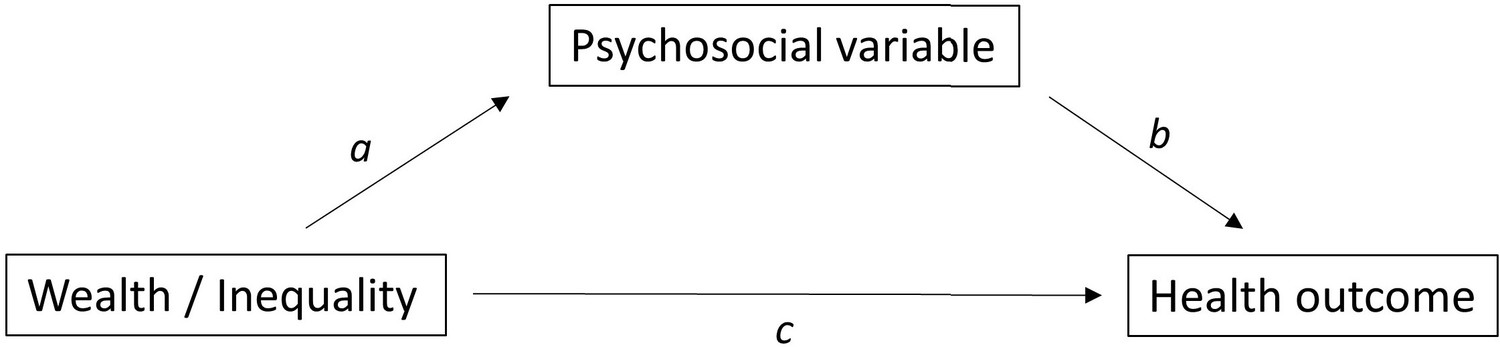
Causal relationships assumed by the mediation analyses.
Appendix 1—figure 2
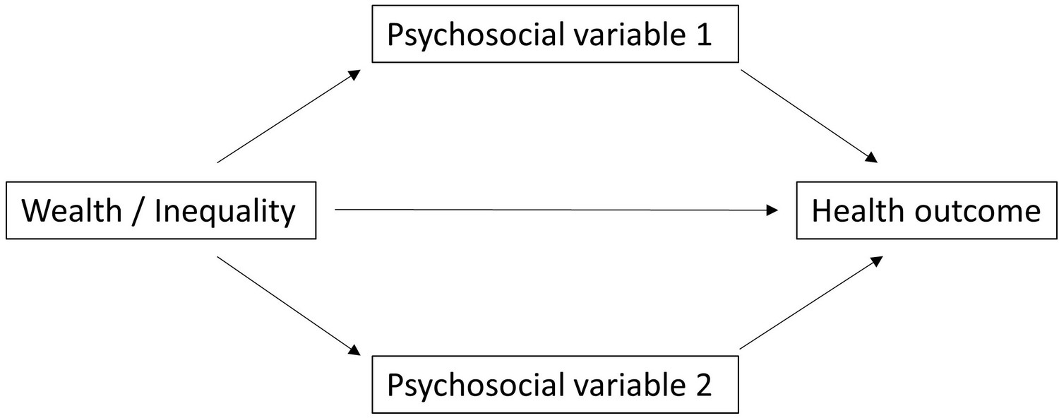
Causal diagram highlighting multiple mediation.
Appendix 1—figure 3
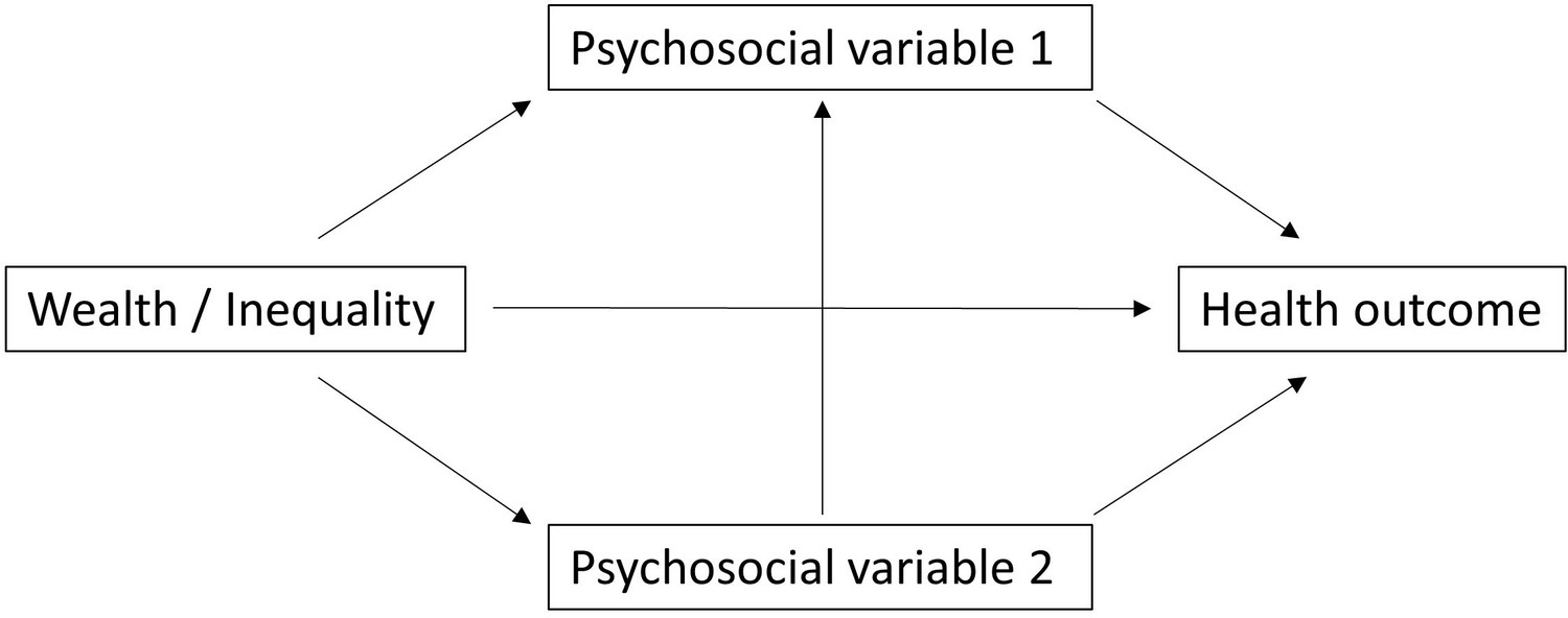
Causal diagram highlighting multiple mediation and collider bias.
Author response image 1
Tables
Table 1
Overview of study variables and descriptive statistics.
For an overview of the sample relative to all people known to the Tsimane Health and Life History Project and at risk of having wealth data, see Figure 1—figure supplement 1.
| Variable | N | Obs | Median | SD | Min | Max |
|---|---|---|---|---|---|---|
| Adult outcomes: psychosocial | ||||||
| Depression (possible range 16–64) | 528 | 670 | 40.0 | 7.1 | 23.0 | 62.0 |
| Conflicts (possible range 0–4) | 342 | 401 | 2.0 | 0.7 | 0.0 | 4.0 |
| Labor partners (count)* | 304 | 399 | 2.0 | 2.0 | 1.0 | 13.0 |
| Non-social problems (possible range 0–7) | 339 | 398 | 3.0 | 1.2 | 0.0 | 7.0 |
| Urinary cortisol (pg/ml) | 588 | 811 | 155,191 | 149,602 | 93 | 851,308 |
| Adult outcomes: health | ||||||
| Body mass index (kg/m2) † | 1901 | 5179 | 23.3 | 2.8 | 16.0 | 36.6 |
| Systolic blood pressure (mmHg) | 1622 | 3195 | 110.0 | 12.8 | 60.0 | 190.0 |
| Diastolic blood pressure (mmHg) | 1622 | 3195 | 70.0 | 10.0 | 24.0 | 136.0 |
| Self-rated health (1 excellent to 5 very bad) | 1307 | 2523 | 4.0 | 0.5 | 1.0 | 5.0 |
| Total morbidity (possible range 0–18)‡ | 1306 | 1542 | 2.0 | 1.1 | 0.0 | 5.0 |
| Infections/parasites (yes/no) ‡ | 1306 | 1542 | 25.2% | |||
| Respiratory disease (yes/no) ‡ | 1306 | 1542 | 21.9% | |||
| Gastrointestinal (yes/no) ‡ | 1306 | 1542 | 36.3% | |||
| Adult predictors | ||||||
| Age (years) | 1931 | 5383 | 35.0 | 15.1 | 16.0 | 91.0 |
| Sex (0 = female, 1 = male) | 1931 | 5383 | 46.2 | |||
| Juvenile outcomes: health | ||||||
| Body mass index (kg/m2) † | 1765 | 4747 | 16.6 | 2.1 | 10.2 | 27.6 |
| Total morbidity (count) ‡ | 1423 | 1569 | 1.0 | 0.8 | 0.0 | 4.0 |
| Infections/parasites (yes/no) ‡ | 1423 | 1569 | 13.6% | |||
| Respiratory disease (yes/no) ‡ | 1423 | 1569 | 42.4% | |||
| Gastrointestinal (yes/no) ‡ | 1423 | 1569 | 41.2% | |||
| Juvenile predictors | ||||||
| Age (years) | 1772 | 4783 | 7.0 | 4.1 | 0.0 | 15.0 |
| Sex (0 = female, 1 = male) | 1772 | 4783 | 49.6 | |||
| Household predictors | ||||||
| Household size | 871 | 1045 | 4.0 | 2.7 | 1.0 | 14.0 |
| Household wealth (Bs) | 871 | 1045 | 7675 | 5675 | 386 | 56,664 |
| Community predictors | ||||||
| Community size (adults > 15) | 40 | 55 | 72.0 | 81.2 | 27.0 | 346.0 |
| Distance to market town (km) | 40 | 55 | 43.0 | 44.2 | 5.0 | 140.0 |
| Mean community wealth (Bs) | 40 | 55 | 8373 | 2331 | 3930 | 16,250 |
| Community wealth inequality (Gini) | 40 | 55 | 0.27 | 0.07 | 0.15 | 0.53 |
-
*
Reverse coded in analyses to make higher values worse outcomes.
-
†
Whether higher or lower body mass index is better is a bit ambiguous: in high-income countries higher body mass index is associated with worse health, lower status, and greater inequality, whereas in low-income countries the reverse may be true.
-
‡
See Table 2 for an overview of the most common morbidities by category.
Table 2
Overview of the most common morbidities.
Three of the most common Clinical Classifications System (CCS) categories (number in parentheses) and the six most prevalent diagnoses within each category (in decreasing order down rows, ICD-10 codes in parentheses). Musculoskeletal conditions (CCS 13) were also common but not analyzed independently.
| Infectious and parasitic diseases(CCS 1) | Diseases of the respiratory system (CCS 8) | Diseases of the digestive system (CCS 9) |
|---|---|---|
| Pediculosis due to Pediculus humanus capitis (B85.0) | Acute nasopharyngitis (common cold) (J00) | Intestinal helminthiasis (B82.0) |
| Tinea unguium (B35.1) | Acute streptococcal tonsillitis; unspecified (J03.00) | Infectious gastroenteritis and colitis (A09) |
| Candidiasis of vulva and vagina (B37.3) | Streptococcal pharyngitis (J02.0) | Dyspepsia (K30) |
| Pediculosis; unspecified (B85.2) | Acute upper respiratory infection; unspecified (J06.9) | Gastro-esophageal reflux disease with esophagitis (K21.0) |
| Superficial mycosis; unspecified (B36.9) | Acute bronchitis due to Mycoplasma pneumonia (J20.0) | Giardiasis (lambliasis) (A07.1) |
| Necatoriasis (B76.1) | Bronchopneumonia; unspecified organism (J18.0) | Gastritis; unspecified, without bleeding (K29.70) |
Additional files
-
Supplementary file 1
This file contains the following tables with additional information on the statistical models.
a: Model summary – depression. b: Model summary – social conflicts. c: Model summary – fewer labor partners. d: Model summary – non-social problems. e: Model summary – cortisol. f: Model summary – BMI. g: Model summary – systolic blood pressure. h: Model summary – diastolic blood pressure. i: Model summary – worse self-rated health. j: Model summary – total morbidity. k: Model summary – infections. l: Model summary – respiratory illness. m: Model summary – gastrointestinal illness. n: Gaussian model summaries for juveniles. o: Logistic model summaries for juveniles. p: Overview of exploratory interaction effects. q: Mediation of wealth effects. r: Mediation of inequality effects. s: Mediation of mean community wealth effects.
- https://cdn.elifesciences.org/articles/59437/elife-59437-supp1-v2.docx
-
Transparent reporting form
- https://cdn.elifesciences.org/articles/59437/elife-59437-transrepform1-v2.pdf
Download links
A two-part list of links to download the article, or parts of the article, in various formats.
Downloads (link to download the article as PDF)
Open citations (links to open the citations from this article in various online reference manager services)
Cite this article (links to download the citations from this article in formats compatible with various reference manager tools)
Do wealth and inequality associate with health in a small-scale subsistence society?
eLife 10:e59437.
https://doi.org/10.7554/eLife.59437


