An ABA-GA bistable switch can account for natural variation in the variability of Arabidopsis seed germination time
- The Sainsbury Laboratory, University of Cambridge, United Kingdom
Figures
Figure 1 with 1 supplement
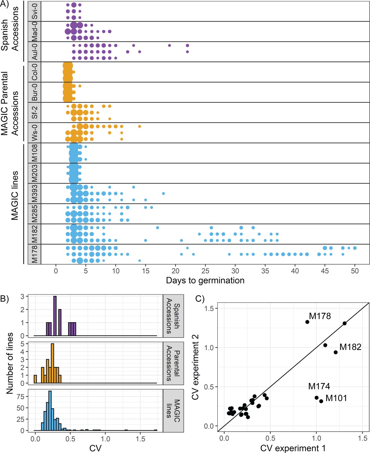
There is variation in variability in germination times in Arabidopsis.
(A) Examples of distributions of germination time for natural accessions and MAGIC lines. Each row shows the germination time distribution of a seed batch from a different parent plant of a particular line, and colours represent whether the line is a Spanish accession (purple), MAGIC parental accession (yellow) or MAGIC line (blue). The size of the circles is proportional to the percentage of seeds sown that germinated on a given day. For the two groups of accessions (Spanish accessions and MAGIC parents), examples of the lowest and highest variability lines are shown. For MAGIC lines, examples are shown of low variability (top two lines); high variability, long-tailed (middle two lines) and very high variability bimodal (bottom two lines) lines. (B) Frequency distribution of coefficient of variation (CV) of germination times for 10 Spanish accessions (purple), the 19 parental natural accessions that were used to generate the MAGIC lines (orange) and 341 MAGIC lines (blue). In the majority of cases, the CV of a given MAGIC line is the mean of the CVs of three batches of seeds collected from separate parent plants. (C) CV of germination times for a subset of 32 MAGIC lines in two separate experiments. The batches of seeds for the two experiments were derived from different independently sown mother plants. The line shows y = x and is for visualisation purposes only (i.e., it does not represent a trend line). Figure 1—figure supplement 1 shows the level of reproducibility of germination time distributions across replicates, lengths of period of dry storage and sowing conditions. Figure 1—source data 1 contains source data for (A). Figure 1—source data 2 contains source data for (B). Figure 1—source data 3 contains source data for (C).
-
Figure 1—source data 1
Figure 1_A_ExampleGermDistributions.
- https://cdn.elifesciences.org/articles/59485/elife-59485-fig1-data1-v1.tds
-
Figure 1—source data 2
Figure 1_B_MAGICsAccessionsTraitSummaries.
- https://cdn.elifesciences.org/articles/59485/elife-59485-fig1-data2-v1.tds
-
Figure 1—source data 3
Figure 1_C_MAGICExperimentComparison.
- https://cdn.elifesciences.org/articles/59485/elife-59485-fig1-data3-v1.tds
Figure 1—figure supplement 1

Reproducibility of germination time distributions.
(A, B) Coefficient of variations (CVs) of germination time for MAGIC parental accession seeds stored in dry conditions for different lengths of time following harvest (x and y axes labels indicate time of storage). Each point represents a different MAGIC parental accession and is the mean CV across three replicate batches of seeds, each collected from a different parent plant. The black lines show y = x to aid data visualisation (they do not represent models fitted to the data). The experimental comparisons are for 16 (A) and 12 (B) of the MAGIC parental accessions. For (A), Pearson’s r = 0.77 (95% CI [0.44, 0.91]). For (B), Pearson’s r = 0.76 (95% CI [0.32, 0.93]). (C–F) Germination time distributions of the very high variability MAGIC lines shown in Figure 1C. Each row shows the germination time distribution of a seed batch from a different parent plant. Each colour represents seeds collected and sown in a single experiment, with different colours representing different replicate experiments from different parental sowings. The size of the circles is proportional to the percentage of seeds that germinated on a given day. M101 and M174 showed a very late germinating fraction of seeds in some experiments but not others, whilst bimodal distributions were more consistently detected for M182 and M178. (G) Distributions of germination times on soil for genotypes that were either high or low variability when sown on Petri dishes. Within an experiment, lines that were more variable on plates were also more variable on soil, with the exception of M311. Figure 1—figure supplement 1—source data 1 contains source data for (A) and (B). Figure 1—figure supplement 1—source data 2 contains source data for (C–F). Figure 1—figure supplement 1—source data 3 contains source data for (G).
-
Figure 1—figure supplement 1—source data 1
Figure1_figure supplement 1_A_B_MagicParentsCVvsDAR.
- https://cdn.elifesciences.org/articles/59485/elife-59485-fig1-figsupp1-data1-v1.tds
-
Figure 1—figure supplement 1—source data 2
Figure1_figure supplement 1_CtoF_HighVarLinesReproducibility.
- https://cdn.elifesciences.org/articles/59485/elife-59485-fig1-figsupp1-data2-v1.tds
-
Figure 1—figure supplement 1—source data 3
Figure1_figure supplement 1_G_SoilvsPlates.
- https://cdn.elifesciences.org/articles/59485/elife-59485-fig1-figsupp1-data3-v1.tds
Figure 2 with 1 supplement
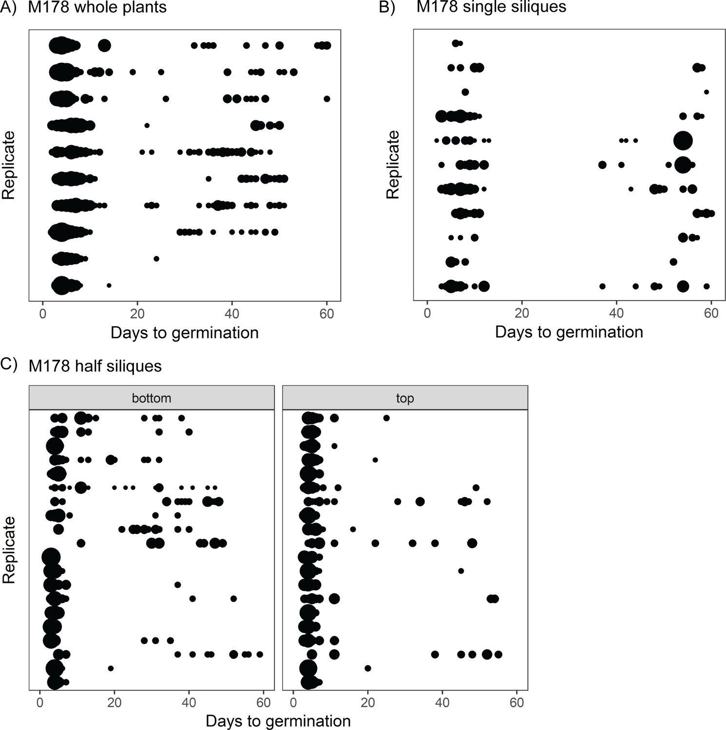
The full range of germination times can be found in individual siliques.
(A) Germination time distributions for a very high variability line, M178. Each row is the distribution obtained using a sample of pooled seeds from one plant, with different rows showing data from different mother plants. (B) As for (A) but each row represents the distribution obtained using seeds from a single silique. Single siliques were randomly sampled from parent plants, and single siliques sampled from seven parent plants are represented. (C) Individual siliques were cut in half, and seeds from the top and bottom halves (distal and proximal, furthest and closest to the mother plants’ inflorescence stems, respectively) were sown separately. Each row is the bottom and top half of a particular silique. Half siliques sampled from two parent plants are represented. Seeds from whole plants, single siliques and half siliques were obtained and sown in different experiments. The size of the circles is proportional to the percentage of seeds that were sown that germinated on a given day. Figure 2—figure supplement 1 shows examples for other MAGIC lines plus an experimental repeat and statistical analysis. Figure 2—source data 1 contains source data for (A). Figure 2—source data 2 contains source data for (B). Figure 2—source data 3 contains source data for (C).
-
Figure 2—source data 1
Figure2_A_M178WholePlant.
- https://cdn.elifesciences.org/articles/59485/elife-59485-fig2-data1-v1.tds
-
Figure 2—source data 2
Figure2_B_M178SingleSiliques.
- https://cdn.elifesciences.org/articles/59485/elife-59485-fig2-data2-v1.tds
-
Figure 2—source data 3
Figure2_C_M178HalfSiliques.
- https://cdn.elifesciences.org/articles/59485/elife-59485-fig2-data3-v1.tds
Figure 2—figure supplement 1

Germination time distributions for whole plants and single siliques for high variability lines.
Germination time distributions for M182 (A) and M53 (B) for samples of seeds pooled from whole plants and for single siliques separated into top and bottom halves. Seeds from whole plants and half siliques were obtained and sown in different experiments. The siliques were randomly sampled from parent plants, and halved siliques from multiple plants are represented (three parent plants for M182 and ten for M53). For whole plants, each row is the distribution obtained using a sample of pooled seeds from one plant. For half siliques, each row is the bottom and top half of a particular silique (top half is that furthest from the mother plant's inflorescence stem). The size of the circles is proportional to the percentage of seeds that were sown that germinated on a given day. (C) As for (A) and (B) but for M4, showing whole siliques in the right-hand panel. Single siliques sampled from eight parent plants are represented. (D) Comparison of seed germination times between top and bottom halves of individual siliques for M182 and M178 MAGIC lines, collected and sown in two independent experiments (exp1 and exp2). Panels show the CV (panel i) and fraction of late germinating seeds (after day 20, panel ii) from the two halves of each assayed silique. Brown lines indicate significant differences from the null hypothesis (<5% false discovery rate). This was determined from bootstrap-based tests that accounted for the unequal number of seeds sown for each silique’s half. Note that even when there is a significant difference between the two silique halves, it is not consistently in the same direction. Figure 2—figure supplement 1—source data 1 contains source data for whole plant germination distributions in (A–C). Figure 2—figure supplement 1—source data 2 contains source data for M182 and M53 half silique germination distributions in (A) and (B). Figure 2—figure supplement 1—source data 3 contains source data for M4 single silique germination distributions in (C). Figure 2—figure supplement 1—source data 4 contains source data for (D).
-
Figure 2—figure supplement 1—source data 1
Figure2_figure supplement 1_AtoC_WholePlant.
- https://cdn.elifesciences.org/articles/59485/elife-59485-fig2-figsupp1-data1-v1.tds
-
Figure 2—figure supplement 1—source data 2
Figure2_figure supplement 1_A_B_M182_M53_halfSiliques.
- https://cdn.elifesciences.org/articles/59485/elife-59485-fig2-figsupp1-data2-v1.tds
-
Figure 2—figure supplement 1—source data 3
Figure2_figure supplement 1_C_M4_singleSilique.
- https://cdn.elifesciences.org/articles/59485/elife-59485-fig2-figsupp1-data3-v1.tds
-
Figure 2—figure supplement 1—source data 4
Figure2_figure supplement 1_D_TopBottomSiliqueComparison.
- https://cdn.elifesciences.org/articles/59485/elife-59485-fig2-figsupp1-data4-v1.tds
Figure 3 with 2 supplements
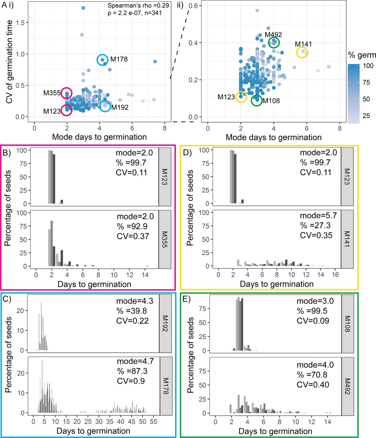
Variability is weakly coupled to modal germination time.
(A) Scatter plots of coefficient of variation (CV) of germination time versus mode days to germination for 341 MAGIC lines. Each point is a specific MAGIC line, and in the majority of cases, the CV and mode are mean values obtained from sowing one batch of seeds from each of three separate parent plants. Each point is shaded according to the percentage germination of the line (see scale bar). Coloured circles and labels indicate lines for which examples are shown in (B–E). (ii) is a zoom in of (i) including only lines with CV < 0.6. Spearman’s correlation for the full set of 341 MAGIC lines is indicated in (i). (B–E) Distributions of germination times for pairs of MAGIC lines. The colour of the box matches the coloured circles in (A). Lower CV lines are shown on top. Grey-coloured bars show the germination time distribution of seed batches from replicate mother plants. (B, C) Exemplar lines with the same mode days to germination but different CVs of germination time. (D, E) Lines that have different CVs and different mode days to germination. For each line, the mode days to germination, final percentage germination and CV of germination time are shown. Note that the x-axis scale differs between plots. Figure 3—figure supplement 1 shows the relationship between CV and percentage germination for MAGIC lines. Figure 3—figure supplement 2 shows relationships between CV, mode and percentage germination for natural accessions. Figure 3—source data 1 contains source data for (A). Figure 3—source data 2 contains source data for (B–E).
-
Figure 3—source data 1
Figure3_AllMAGICsTraitSummaries.
- https://cdn.elifesciences.org/articles/59485/elife-59485-fig3-data1-v1.tds
-
Figure 3—source data 2
Figure3_MAGICIndividualLinesGermPerDay.
- https://cdn.elifesciences.org/articles/59485/elife-59485-fig3-data2-v1.tds
Figure 3—figure supplement 1

Variability is weakly coupled to percentage germination.
(A) Scatter plots of coefficient of variation (CV) of germination time versus percentage germination for 341 MAGIC lines. Each point is a specific MAGIC line, and in the majority of cases, the CV and percentage are mean values for three batches of seeds from separate parent plants. Coloured circles and labels indicate lines for which examples are shown in (B, C). (ii) is a zoom in of (i), including only lines with CV < 0.6. Spearman’s correlation for the full set of 341 MAGIC lines is indicated in (i). (B, C) Distributions of germination times for exemplar MAGIC lines that have similar final percentage germination and mode days to germination but different CVs. The colour of the box matches the lines to the coloured circles in (A). Lower CV lines are shown on top. Grey-coloured bars show the distribution of germination time for seed batches from replicate mother plants. Note that the x-axis scale differs between (B) and (C). Figure 3—source data 1 contains source data for (A). Figure 3—source data 2 contains source data for (B) and (C).
Figure 3—figure supplement 2
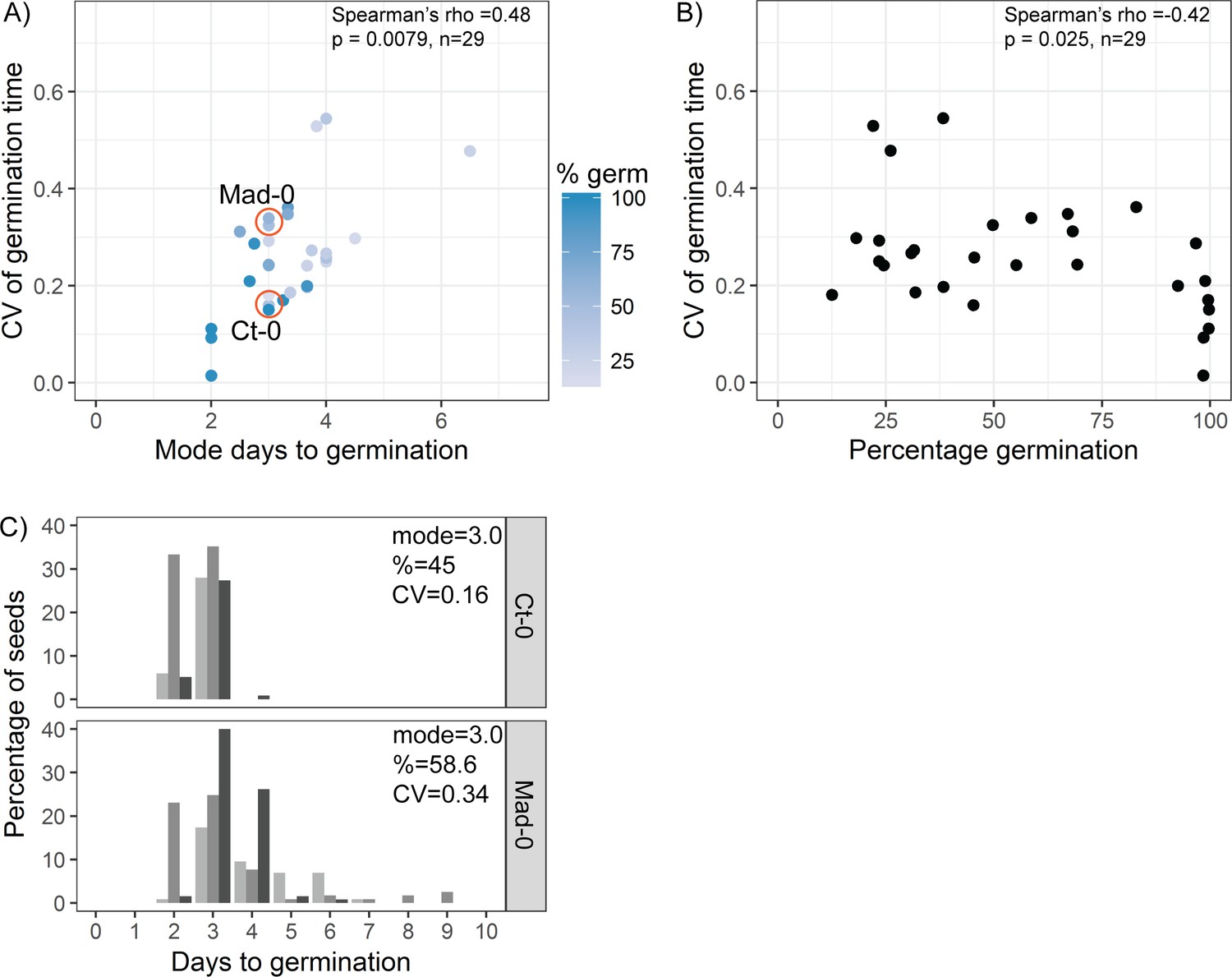
The relationship between coefficient of variation (CV), mode days to germination and percentage germination in natural accessions.
(A) Scatter plot of CV of germination time versus mode days to germination for the 19 parental accessions of the MAGIC lines and 10 Spanish accessions. Each point is a specific accession, and the CV and mode are means for one batch of seed from each of at least three separate parent plants. Each point is shaded according to the percentage germination of the line (see scale bar). Orange circles indicate lines for which examples are shown in (C). Spearman’s correlation for the 29 accessions is indicated. (B) As for (A), but showing CV versus percentage germination. (C) Distribution of germination times for exemplar accessions, with similar mode and percentage germination but different CVs (accessions indicated in A). Grey-coloured bars show the distributions of germination for seed batches from replicate mother plants. Figure 3—figure supplement 2—source data 1 contains the source data for (A) and (B). Figure 3—figure supplement 2—source data 2 contains the source data for (C).
-
Figure 3—figure supplement 2—source data 1
Figure3_figure supplement 2_A_B_AccessionsTraitSummaries.
- https://cdn.elifesciences.org/articles/59485/elife-59485-fig3-figsupp2-data1-v1.tds
-
Figure 3—figure supplement 2—source data 2
Figure3_figure supplement 2_C_AccessionsCt_Mad_GermPerDay.
- https://cdn.elifesciences.org/articles/59485/elife-59485-fig3-figsupp2-data2-v1.tds
Figure 4 with 5 supplements
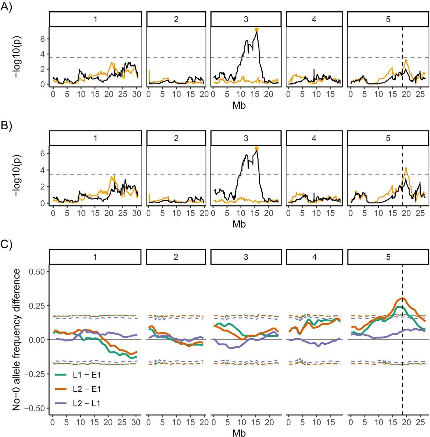
Quantitative trait locus (QTL) and bulk segregant mapping reveals two QTL underlying coefficient of variation (CV) of germination time.
(A, B) Manhattan plots showing the QTL association results for each single nucleotide polymorphism (SNP) marker individually (black line) and for each marker when the Chr3 QTL SNP marker was added as a covariate (i.e. an additional variable) in the model (orange line). The orange line shows the variation in CV that is accounted for by each SNP across the genome when the variation that is explained by the Chr3 QTL SNP marker (orange point) is accounted for by adding it to the model as a covariate. The y-axis shows the p-values for the 1254 markers used, on a negative log10 scale, such that higher peaks indicate a stronger association between the region of the genome and CV. The numbered panels represent the five chromosomes of Arabidopsis. The horizontal dashed line shows a 5% genome-wide threshold corrected for multiple testing (based on simulations in Kover et al., 2009). The vertical dashed line indicates the DOG1 gene. (A) is for the full set of 341 MAGIC lines that was phenotyped and (B) excludes the eight bimodal lines with very high CV. Figure 4—figure supplement 1 shows QTL mapping for mean and mode days to germination and percentage germination. Figure 4—figure supplement 2 shows estimated effects of accession haplotypes on CV, mode and percentage germination. (C) Mapping QTL by bulk-segregant analysis using whole-genome pooled sequencing of F2 pools from a Col-0 × No-0 cross. One early and two late germinating F2 pools were sequenced. The plot shows the No-0 allele frequency differences between pairs of pools indicated in the legend (Figure 4—figure supplement 3 shows details of pool selections; E1, "early pool"; L1, "late one pool"; L2, "late two pool"). The horizontal dashed lines indicate the 95% thresholds based on simulating the null hypothesis of random allele segregation, taking into account the size of the sampled pools and the sequencing depth at each site (Magwene et al., 2011; Takagi et al., 2013). Positive values above the top line indicate enrichment for No-0 alleles, while negative values below the bottom line indicate enrichment for Col-0 alleles. As predicted, late germinating pools were enriched for the No-0 haplotype in the region of the Chr5 QTL. Here, the peak of association overlaps with the DOG1 gene (dashed vertical line). Figure 4—figure supplement 4 shows germination phenotypes of F3 seeds from Col-0 x No-0 F2 plants that themselves germinated early or late.
Figure 4—figure supplement 1
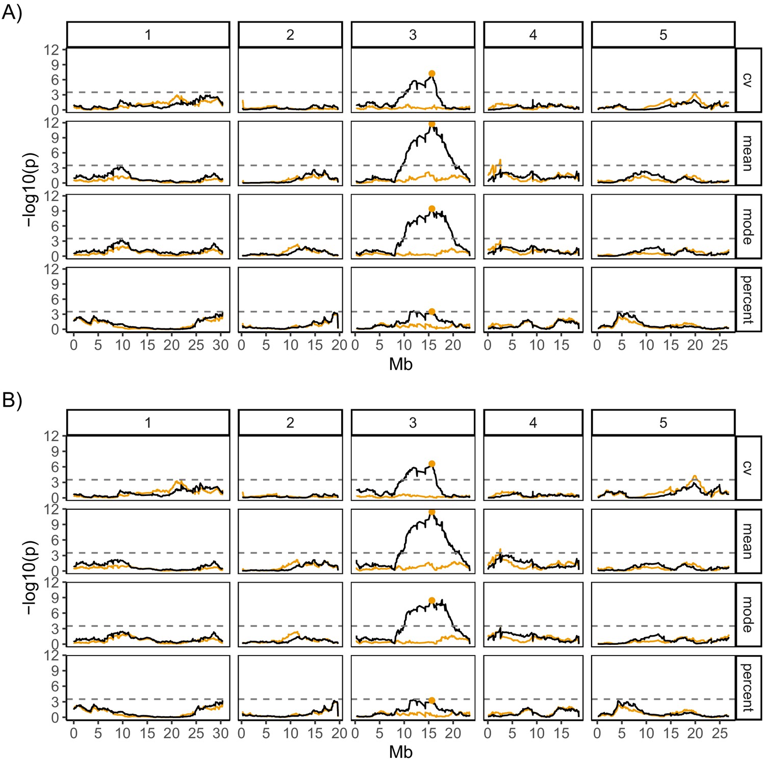
Quantitative trait locus mapping for germination traits, with and without bimodal MAGIC lines.
(A) is for all 341 MAGIC lines that were phenotyped, and (B) is for 333 of these lines (the full set minus the eight bimodal lines with very high coefficient of variation [CV]). The y-axis shows the p-values for the 1254 markers used, on a negative log10 scale. The numbered panels represent the five chromosomes of Arabidopsis, and the scan was performed for four germination traits: CV of germination time, mean germination time, mode germination time and percentage germination. The horizontal dashed line shows a 5% genome-wide threshold corrected for multiple testing (based on simulations in Kover et al., 2009).
Figure 4—figure supplement 2
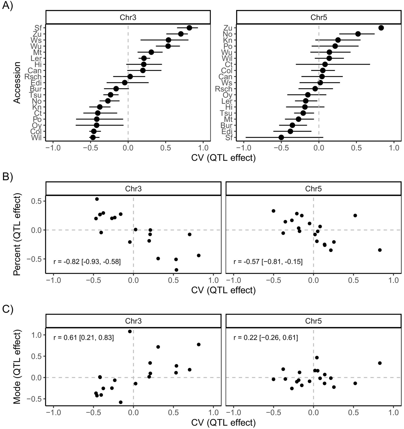
Accession-specific quantitative trait locus (QTL) effects on coefficient of variation (CV), mode and percentage germination.
(A) Predicted accession effects at the two putative QTL on Chr3 and Chr5 (Figure 4). The effects of the 19 parental accession haplotypes were estimated by calculating the mean CV of MAGIC lines inferred to carry each particular haplotype. (B) Correlation between predicted QTL effects on percentage germination and CV. (C) Correlation between predicted QTL effects on mode days to germination and CV. In all panels, the mean effect of each parental accession’s QTL allele was estimated from the probabilistic assignment of each MAGIC line to that founder parent (Kover et al., 2009). Error bars in (A) show the 95% confidence intervals of these estimates (these were omitted from the other panels for clarity). All trait values were standardised, so that axis units represent the number of standard deviations away from the respective mean, with the horizontal and vertical dashed lines at zero highlighting the mean of the respective trait in the population. Pearson’s correlation, r, is indicated in each panel in B and C, with the 95% confidence interval in brackets.
Figure 4—figure supplement 3
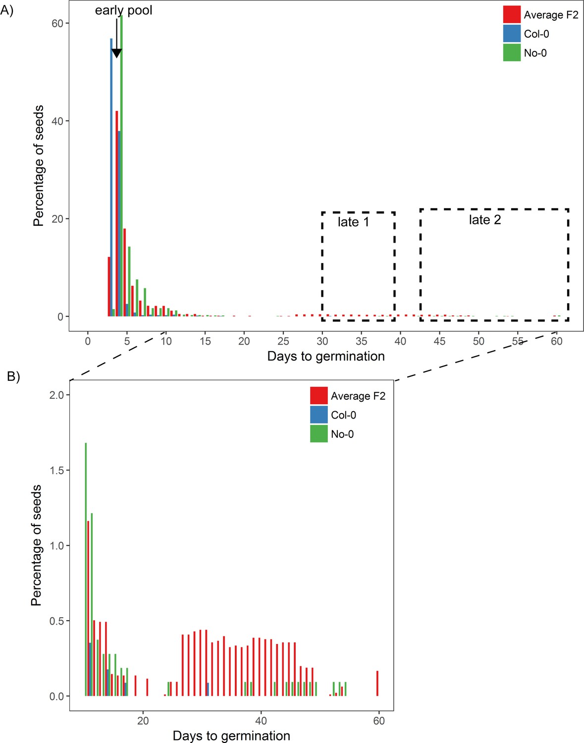
Germination time distributions and DNA-seq pools of Col-0 × No-0 F2.
Eight batches of Col-0 × No-0 F2 seeds, each containing ~1100 seeds and collected from a different F1 parent plant, were sown on soil. Seeds from parental accessions Col-0 and No-0 were also included in the experiment, and, for these, batches of ~1100 seeds pooled from three parent plants were sown for each accession. The different F2 batches behaved similarly, so here we present an averaged (mean) distribution based on bulked data. The percentage germination each day is a percentage of all seeds that germinated (rather than of all seeds that were sown). (A) shows the full germination time distribution with pools used for DNA sequencing highlighted, and (B) shows days 10–60, with a different y-axis scale to show the late germinating seeds. The 'early pool' used for sequencing was composed of 152 individuals that germinated on day 4; the ‘late 1’ pool was composed of 321 individuals that germinated between days 31 and 39, and the ‘late 2’ pool was composed of 213 individuals that germinated between days 43 and 60. We reasoned that, since late germination is predominantly restricted to the more variable parent (No-0), late germinating F2 plants should be enriched for the No-0 accession at loci promoting high variability (including the Chr5 locus at ~20 Mb, where the No-0 haplotype is predicted to promote high CV). Figure 4—figure supplement 3—source data 1 contains the source data for (A) and (B).
-
Figure 4—figure supplement 3—source data 1
Figure4_FigureSupplement3_A_B_ColNoMappingF2_GermDistributions.
- https://cdn.elifesciences.org/articles/59485/elife-59485-fig4-figsupp3-data1-v1.tds
Figure 4—figure supplement 4
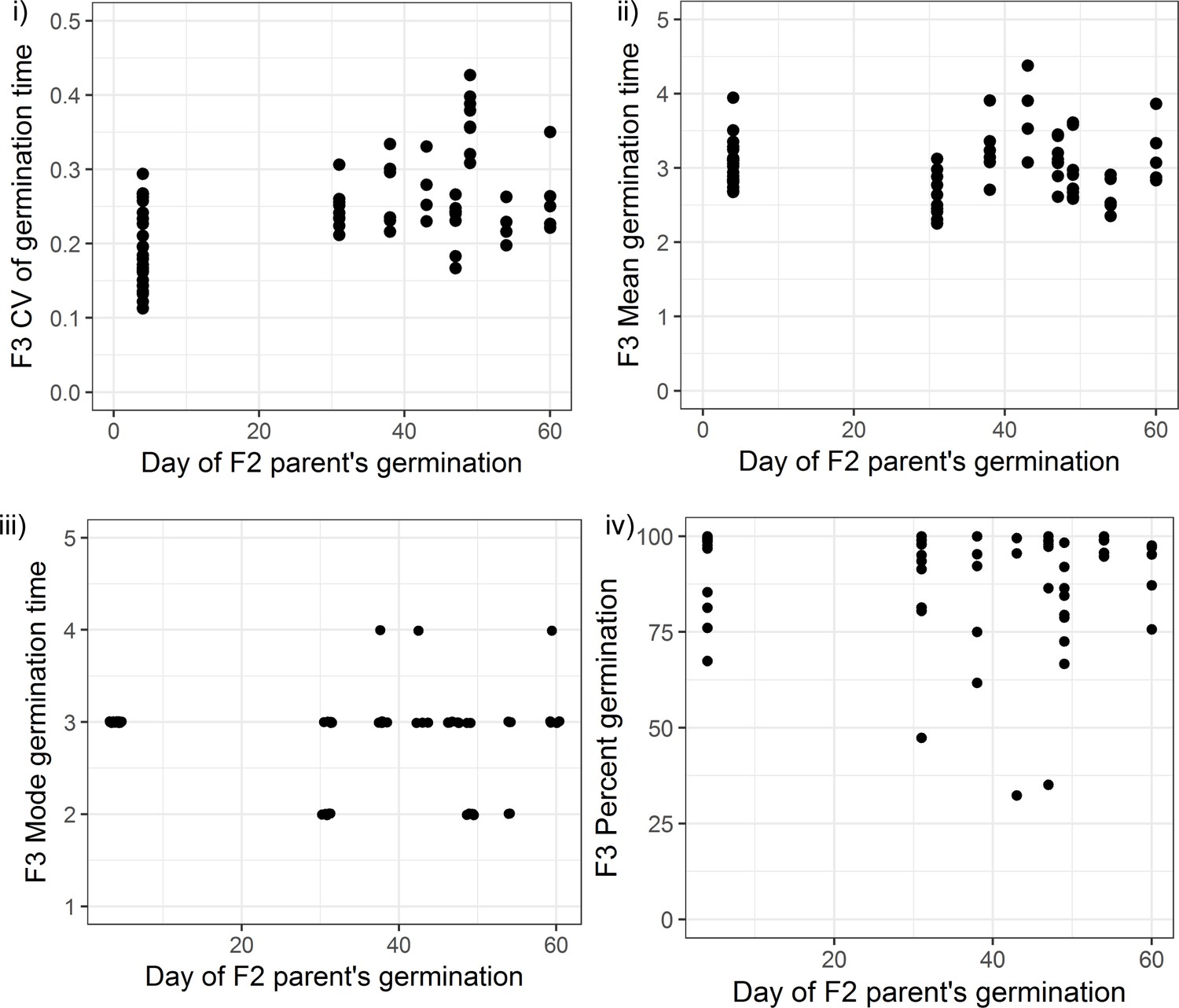
Germination phenotypes of F3 seeds from Col-0 × No-0 F2 parent plants that themselves germinated early or late.
Coefficient of variation (CV) (i), mean (ii), mode (iii) and percentage germination (iv) for F3 seed batches collected from F2 plants that themselves germinated at different times (x-axis). Batches of seeds from F2 plants that germinated late (between days 30 and 60) had, on average, a significantly higher CV than seeds from plants that germinated early (on day 4) (the mean CVs of the two groups were 0.19 in the early group versus 0.27 in the late group, Wilcoxon rank-sum test W = 199, p-value=1.163e-05, n = 23 seed batches from early germinators, n = 47 seed batches from late germinators). Seeds of late germinating plants did not tend to have higher mean or mode germination times (the mean of mean germination times was 3.05 days in the early group versus 3 days in the late group; the mean of mode germination times was 3.00 in the early group versus 2.78 in the late group). Percentage germination shows a small but significant difference between the two groups of F3 seeds (mean percentage germination: 95.3 in the early group versus 87.67 in late group, Wilcoxon rank-sum test W = 754, p-value=0.00419, n = 23 seed batches from early germinators, n = 47 seed batches from late germinators). Each seed batch is from a separate F2 plant. Figure 4—figure supplement 4—source data 1 contains the source data for all panels.
-
Figure 4—figure supplement 4—source data 1
Figure4_FigureSupplement4_ColNoF3_GermDistributions.
- https://cdn.elifesciences.org/articles/59485/elife-59485-fig4-figsupp4-data1-v1.tds
Figure 4—figure supplement 5
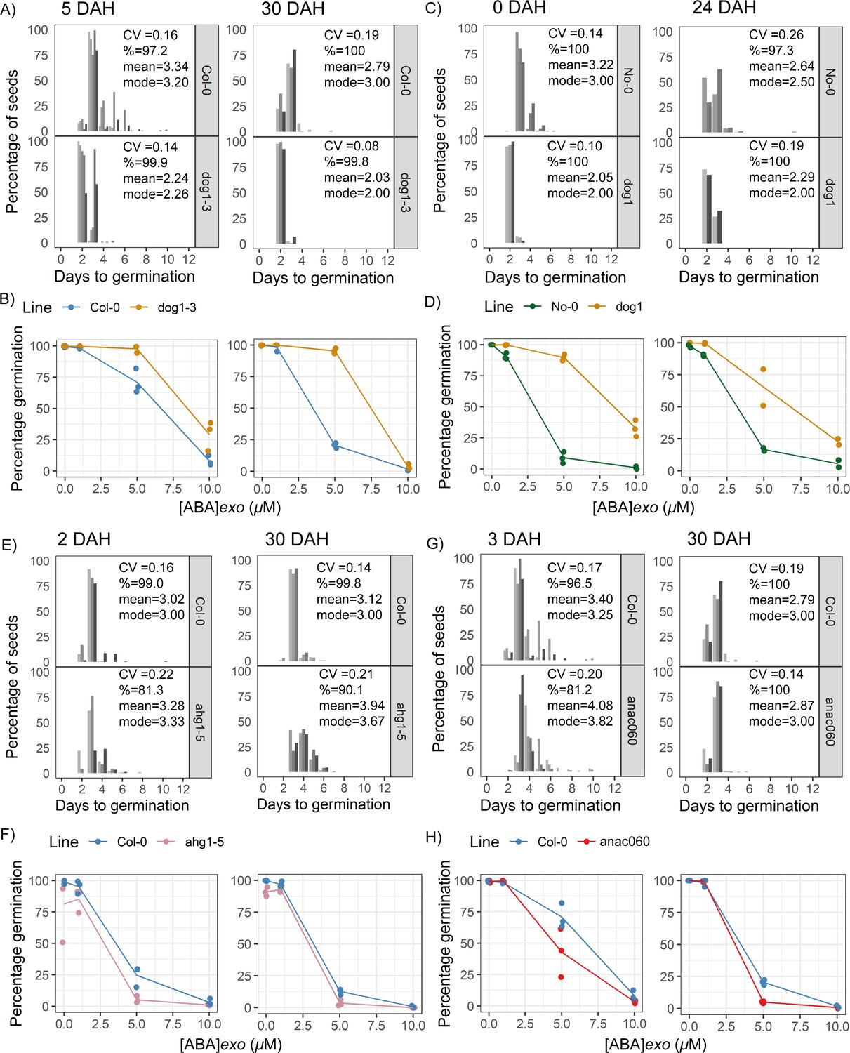
Germination time distributions and abscisic acid (ABA) dose responses in quantitative trait locus candidate gene mutants.
(A, B) dog1-3 mutant in the Col-0 background, for seeds that were 5 days after harvest (DAH) (left panels) or 30 DAH (right panels). Histograms show germination time distributions for replicate seed batches from separate parent plants (shades of grey) of each genotype. The mean of the coefficient of variation of germination time for the different seed batches is displayed on the panels (along with the mean across batches of percentage germination, mode days to germination and mean days to germination). (B) shows an ABA dose response for the wild type and mutant, with three replicate seed batches (dots) for each genotype. The lines join the mean percentages of germination for each treatment for a particular line. (C, D) As for (A, B), but for a dog1 T-DNA mutant in the No-0 background. Here the No-0 control represents wild-type plants obtained from the segregating T-DNA population (see Materials and methods for details). The number of days of seed storage before sowing is shown above each panel. (E, F) As for (A, B), but for the ahg1-5 mutant in the Col-0 background. (G, H) As for (A, B), but for the anac060 mutant in the Col-0 background. In all experiments at least three separate replicate seed batches from separate parent plants were sown for each genotype, except in C, for 24 DAH, where only 2 replicates were used. In the histograms shown in (A) for 5 DAH and in (G) for 3 DAH, five and four separate experiments, respectively, were performed (each with three seed batches). In these cases, each shade of grey is the germination time distribution from a single experiment, with the behaviours of its three separate seed batches pooled together for plotting, treated as one sample. For all other histograms, one experiment was performed and shades of grey are separate replicate seed batches harvested and sown in that single experiment. Source data is provided in Figure 4—figure supplement 5—source data 1.
-
Figure 4—figure supplement 5—source data 1
Figure4_FigureSupplement5_QTLcandidateMutantsGerm.
- https://cdn.elifesciences.org/articles/59485/elife-59485-fig4-figsupp5-data1-v1.tds
Figure 5 with 5 supplements
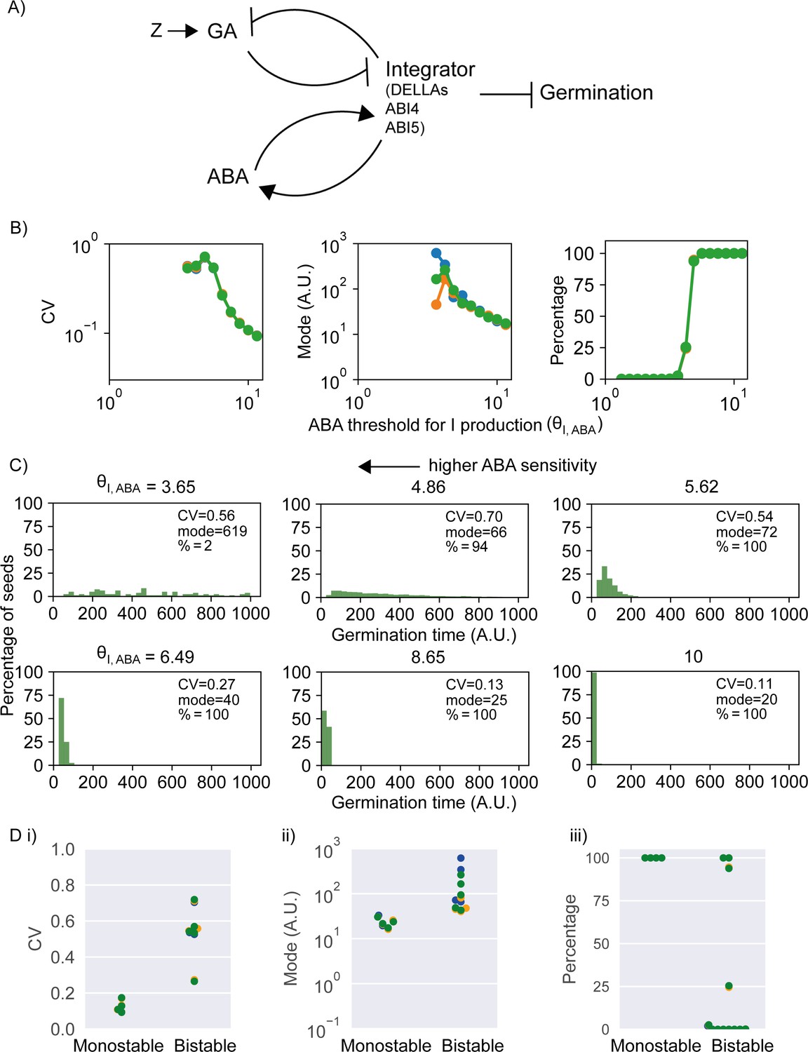
Model of the abscisic acid–gibberellic acid (ABA-GA) bistable switch and effect of ABA sensitivity parameter on germination traits.
(A) Model scheme of the ABA-GA network. Normal arrows represent effective promotion and blunt arrows represent effective inhibition. We represent the inhibitors of germination – DELLAs, ABI4 and ABI5 – as one factor, called Integrator, which we assume must drop below a threshold for germination to occur. We assume that ABA promotes the production of Integrator and that GA promotes its degradation. Integrator is assumed to promote ABA production and inhibit GA production. A factor, Z, increases upon sowing and promotes GA production. Figure 5—figure supplement 1 provides information on the dynamics of the model. (B) Effects on coefficient of variation (CV), mode and percentage germination of simulated germination time distributions as the ABA threshold for Integrator (I) production parameter values are changed. This parameter is inversely correlated with sensitivity of Integrator to ABA. Each panel shows the results of three different runs of stochastic simulations on 4000 seeds. (C) Simulated germination time distributions for six values of the ABA threshold for Integrator production parameter, showing positively correlated changes in CV and mode. The arrow indicates increasing sensitivity of Integrator production to ABA towards the top left. (D) CV, mode and percentage germination in bistable and monostable regions of the model parameter space after the rise in GA production (see Figure 5—figure supplement 1 for details of monostable and bistable regimes). See Materials and methods for regions of the parameter space that we exclude from these plots because they are considered less biologically relevant. Colours in (B) and (D) represent different runs of stochastic simulations. See Materials and methods for further details on parameters and numerical simulations.
Figure 5—figure supplement 1
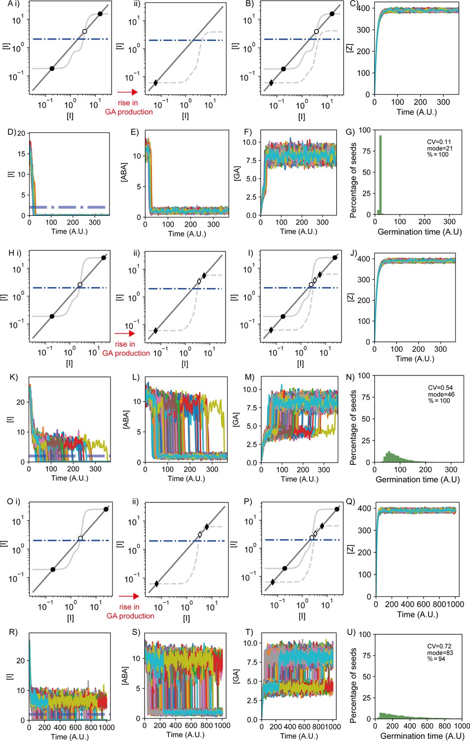
Dynamics of the components of the abscisic acid–gibberellic acid (ABA-GA) model in monostable and bistable regimes.
Modelling results showing representative behaviour of the model when it is in the monostable (A–G) and two bistable scenarios (H–U) after the rise of GA production (referred to as monostable and bistable scenarios for simplicity). (H–N) show a bistable scenario where the non-germination steady state is less stable than the second bistable scenario shown in (O–U). The three scenarios differ in the ABA threshold for integrator production, which modulates ABA sensitivity: the monostable scenario in (A–G) has the highest value of this parameter (θI,ABA = 10), and therefore lowest ABA sensitivity, the first bistable scenario in (H–N) has an intermediate ABA sensitivity (θI,ABA = 5.6) and the second bistable scenario in (O–U) has the highest ABA sensitivity (θI,ABA = 4.87). The bistable scenarios correspond to the grey region in the phase diagrams shown in Figure 5—figure supplement 4, and the monostable scenario corresponds to the white regions. (A, H, O) Results from nullcline analysis for the Integrator variable showing the steady states of the dynamics before (i) and after (ii) the GA production increase (see Materials and methods). In each panel, steady-state solutions are shown by the intersections between the dark grey line and the light grey line. Filled dots and diamonds represent the Integrator stable steady states before and after the GA production increase, respectively. Empty dots and diamonds represent unstable steady states. The dashed-dotted blue line illustrates the Integrator threshold below which germination happens. Before the increase of GA production, the modelled network exhibits a high Integrator stable steady state above the threshold (higher filled dot), representing a non-germinating state before sowing. We set this state as the initial condition of the simulation. For these parameter values, a lower Integrator stable solution below the germination threshold exists (lower filled dot), therefore representing a germination state, as well as an intermediate unstable Integrator solution (empty dot). Hence, bistability occurs for the Integrator variable before the increase of GA production. With the provided noise intensity for these simulations, none of the seeds is able to switch from the non-germination state to the germination state before the rise of GA production in the three scenarios (A), (H) and (O) (see Materials and methods). (Aii) In the monostable scenario after the rise in GA production, the increase in GA production leads to the disappearance of the non-germination state and the unstable steady state through a saddle node bifurcation; this makes the germination state the only possible stable state. (Hii, Oii) In the bistable scenarios after the rise in GA production, the non-germination state (high Integrator, high ABA and low GA) approaches the unstable steady state (empty dot), becoming less stable. In these cases, stochastic fluctuations enable the simulated seeds to cross the unstable steady state, reaching the germination state (low Integrator, low ABA and high GA), which becomes a more stable solution. (B, I, P) Nullclines analyses shown in (A), (H) and (O) subpanels, with the scenarios before and after the rise in GA production represented together. For each panel, the light grey solid line and dots show the case before the rise in GA production, and the light grey dashed line and diamonds show the case after the rise in GA production. (C–F, J–M, Q–T) Time courses for the components of the model in example simulations. Different coloured lines represent different seeds. (C, J, Q) Time courses of the concentration of the factor Z, which increases rapidly upon sowing and promotes GA production. (D, K, R) Time courses of Integrator concentrations. Dashed-dotted blue lines show the threshold below which Integrator must drop for germination to occur. (E, L, S) Time courses of ABA concentrations. (F, M, T) Time courses of GA concentrations. (G, N, U) Histograms of germination times, with values for coefficient of variation, mode and percentage germination of the distribution. Note that the x-axis range for the time courses and histograms is larger for (Q–U) due to the highly variable germination times in this scenario. The simulations representing the bistable scenarios show a transient in which the seeds can remain in a high Integrator state until the stochastic fluctuations cause them to switch to the low Integrator state. Conversely, in the monostable scenario, the seeds achieve the low Integrator state in a more direct manner. See Materials and methods for further details on parameters and numerical simulations.
Figure 5—figure supplement 2
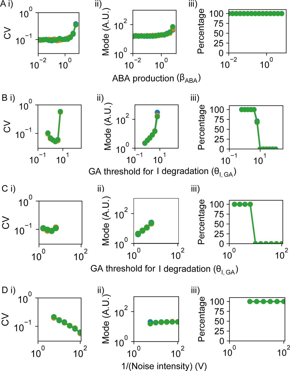
Effect of model parameters on germination traits.
(A–D) show the effects on coefficient of variation (CV), mode and percentage germination of simulated germination time distributions as single parameter values are changed. Each panel shows the results of three different runs of stochastic simulations on 400 seeds, represented in different colours. (A) Varying the rate of abscisic acid (ABA) production as an example of a parameter that, when changed, tends to have positively correlated effects on CV and mode of germination time. (B) Varying the threshold of gibberellic acid (GA) for degradation of Integrator (this parameter is inversely correlated with sensitivity of Integrator to GA). For some points in parameter space, varying this parameter has anti-correlated effects on CV and mode. (C) As for (B), but in a different region in parameter space (see below for parameter details), in which increasing the threshold of GA for degradation of Integrator causes an increase in mode with relatively constant CV which indicates decoupled effects on CV and mode. (D) Varying the effective system volume parameter, V, which controls the level of noise in the system (we define noise intensity as being proportional to 1/V), also causing decoupled effects on CV and mode. For some areas of parameter space, an increase in V, and therefore a decrease in noise, causes the CV to decrease but leaves mode and percentage germination relatively unchanged. Parameter values are provided in the Materials and methods (Table 2) and were the same across simulations with the exception of the parameters varied on x-axes and differences in vABA in (A), V in (B) , θI,ABA in (C) and in (D). See Materials and methods for regions of the parameter space that we exclude from these plots because they are considered less biologically relevant. Figure 5—figure supplement 3 shows simulated germination time distributions corresponding to the parameter explorations in (A–D). Figure 5—figure supplement 4 shows the full results of the 2D parameter screen in terms of the effects of parameter pairs on CV, mode and percentage germination.
Figure 5—figure supplement 3
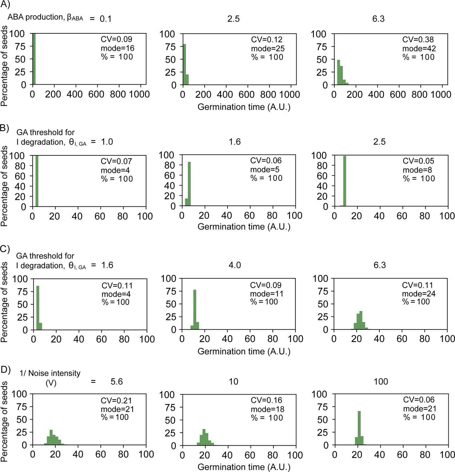
Simulated germination time distributions illustrating the effects of parameter value changes.
Histograms in (A), (B), (C) and (D) correspond to points in the plots in Figure 5—figure supplement 2 from (A), (B), (C) and (D), respectively. (A) Simulated germination time distributions for three values of abscisic acid (ABA) basal production, showing positively correlated changes in coefficient of variation (CV) and mode. (B) As for (A), but varying the gibberellic acid (GA) threshold for Integrator degradation (which is inversely proportional to Integrator sensitivity to GA), illustrating anti-correlated changes in mode and CV. (C) As for (B) but varying the GA threshold for Integrator degradation in an area of parameter space where the mode increases while the CV remains relatively constant. (D) As for (A) but varying the parameter V which governs the level of noise in the system, illustrating a change in CV while the mode remains relatively constant.
Figure 5—figure supplement 4
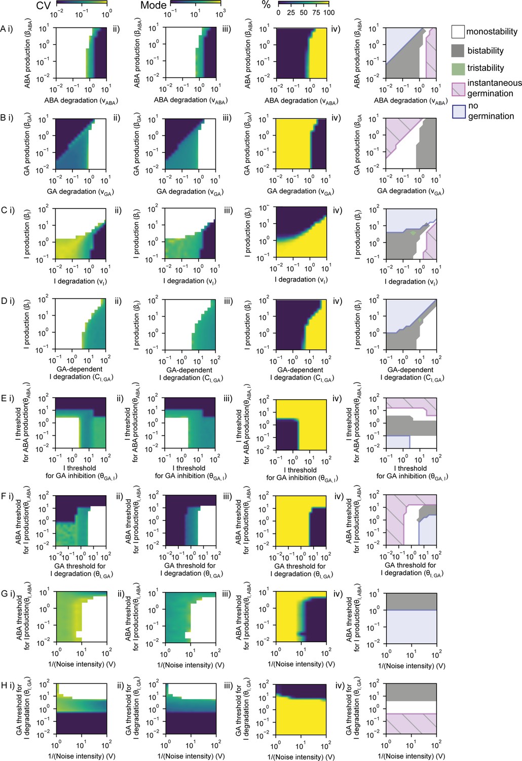
Exploring the effects of model parameters on coefficient of variation (CV), mode and percentage germination.
Each panel shows a result from a 2D parameter exploration for a pair of parameters, such that each parameter is varied for a range of values of a second parameter. (A) Effect of abscisic acid (ABA) basal production and ABA basal degradation parameters on CV (i), mode (ii) and percentage germination(%) (iii) of simulated germination distributions. CVs below 0.01 and above 1 are represented as being 0.01 and 1, respectively. CV and mode of the simulations were represented when there were more than nine seeds germinating out of 1000. (iv) Phase diagram showing theoretically predicted regions from nullcline analysis of the deterministic system: bistability (grey, see Figure 5—figure supplement 1B for information on this region) and tristability (green) regions in which we can expect the full range of behaviours in terms of germination percentage, region where we expect to have all seeds germinated instantaneously (pink hatched), and region where no seeds are expected to germinate in the deterministic limit (i.e. when there is no noise) (blue). The remaining white region is monostable, and we expect all seeds (non-instantaneously) to germinate (see Figure 5—figure supplement 1A, B for information on this region). We expect that just the bistable and tristable scenarios will allow a percentage of seeds to germinate that differs from 0% and 100%. The colour bars above (A) apply to all rows. All rows are as for (A), but exploring the following parameter pairs: (B) Gibberellic acid (GA) basal degradation versus GA basal production; (C) Integrator basal degradation versus Integrator basal production; (D) GA-dependent degradation of Integrator versus Integrator basal production; (E) threshold of Integrator for the inhibition of GA production (which is inversely correlated with sensitivity of GA to Integrator) versus threshold of Integrator for the promotion of ABA production (which is inversely correlated with sensitivity of ABA to Integrator); (F) threshold of GA for the GA-mediated degradation of Integrator (which is inversely correlated with sensitivity of Integrator to GA) versus threshold of ABA for the promotion of Integrator production (which is inversely correlated with sensitivity of Integrator to ABA); (G) effective volume of the system, V (which is inversely proportional to the noise in the system, see Materials and methods), versus threshold of ABA for the promotion of Integrator production; (H) effective volume of the system, V, versus threshold of GA for the degradation of Integrator. The theoretically predicted areas from nullclines (right panels) are closely predictive of the stochastic simulation outcomes (see Materials and methods). Figure 5—figure supplement 5 shows an analysis of the CV, mode of germination times and percentage germination in monostable and bistable regions of these parameter spaces. See Materials and methods for further details of the simulations and theoretical predictions and see Table 2 for full parameter values for each simulation.
Figure 5—figure supplement 5

Coefficient of variation (CV), mode of germination times and percentage germination in bistable and monostable regions of the model after the rise in GA production.
Simulation results across the different 2D parameter explorations shown in Figure 5—figure supplement 4A—G. In panels (A)-(G), points represent simulation results for different combinations of parameter values for the parameter pair indicated on the right. Panels show: i) CV, ii) mode and iii) percentage germination of simulated germination time distributions. Colours represent different runs of stochastic simulations. This analysis focuses on biologically relevant points falling within the monostable and bistable regions (see Materials and methods regarding the excluded, less biologically relevant points). We obtained a similar result in relation to simulations shown in Figure 5—figure supplement 4H but have ommited this here for simplicity.
Figure 6 with 4 supplements
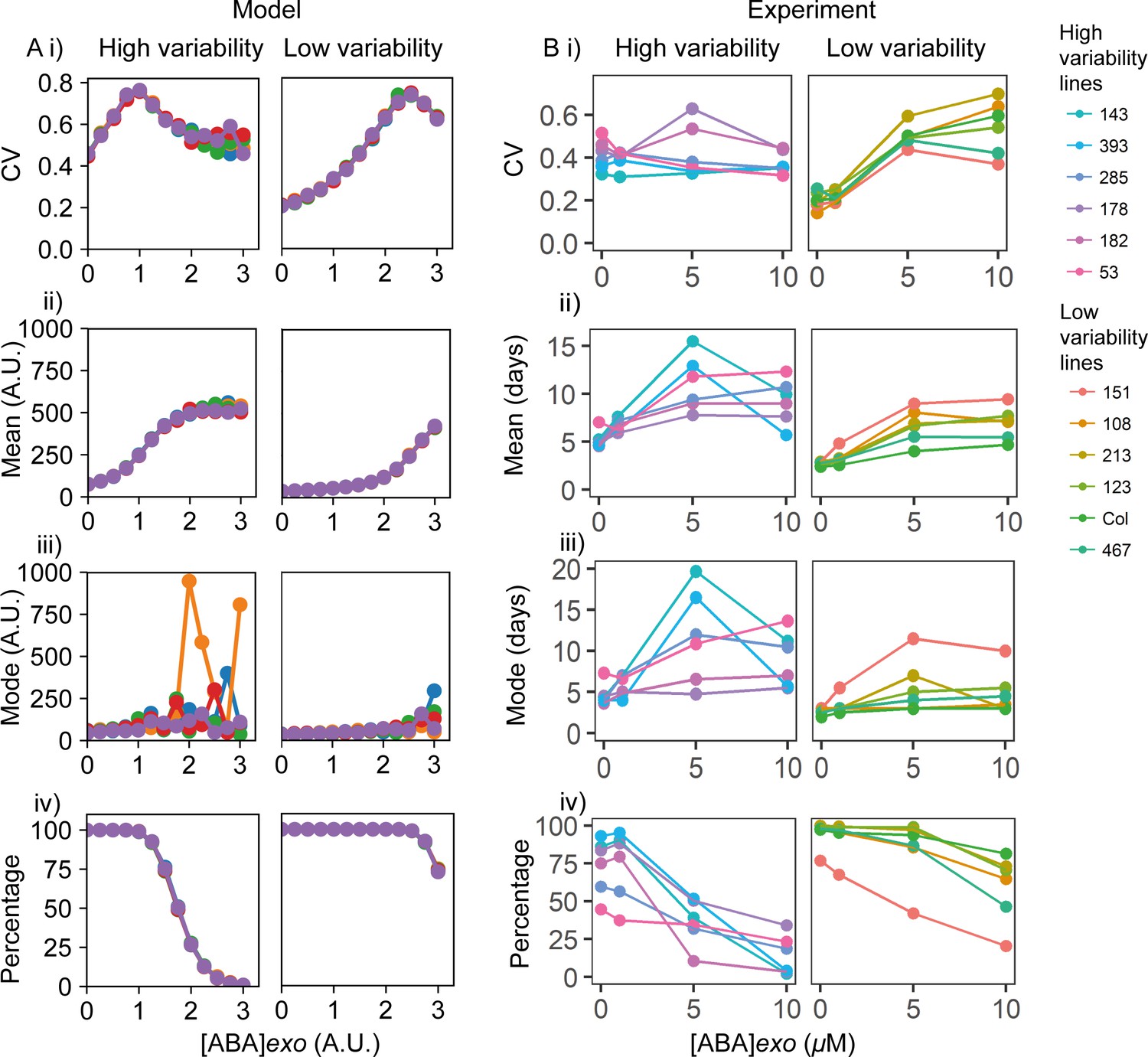
Exogenous addition of abscisic acid (ABA) to high and low variability lines.
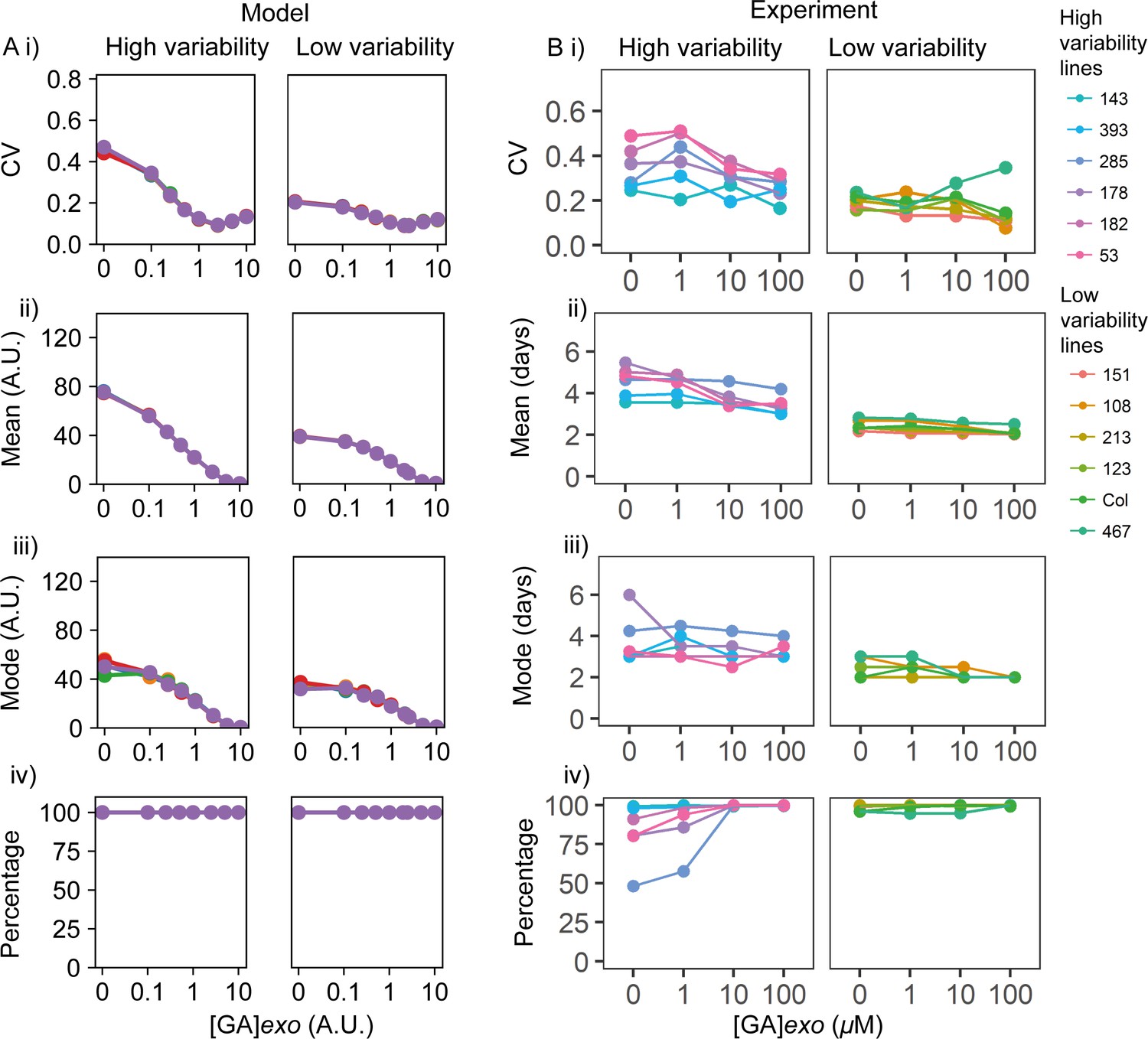
(A) Simulations of addition of increasing doses of exogenous ABA (x-axes), starting from a point in the parameter space that shows higher seed germination time variability (left) and lower variability (right) when no exogenous ABA is added. High variability in seed germination time is simulated with a lower value of the ABA threshold for I production (θI,ABA ) (i.e. higher ABA sensitivity) than low variability in seed germination time. Plots show the effects on the coefficient of variation (CV) (i), mean (ii), mode (iii) and percentage of seeds that germinated (iv) for the resulting germination time distributions. Each panel shows the result of five stochastic simulations for 4000 seeds, each plotted in a different colour. Parameter values for the high and low variability lines simulations are the same with the exception of the ABA threshold for I production (θI,ABA = 7 for the low variability lines and θI,ABA = 5.8 for the high variability lines). See Materials and methods for further simulation details and parameter values. (B) Experimental ABA dose response for six high variability MAGIC lines (left) and six low variability lines (five MAGIC lines plus Col-0) (right). (B) (i) shows mean CVs of individual lines for different exogenous ABA concentrations (means are of at least two independent experiments), (ii) as for (i) but for mean days to germination, (iii) mode days to germination and (iv) percentage germination. Treatments with ‘0’ μM are vehicle control treatments. Figure 6—figure supplement 1 shows exogenous addition of gibberellic acid (GA) in the model and experimentally to the high and low variability lines. Figure 6—figure supplement 2 shows simulated germination time distributions for selected concentrations of exogenous ABA and GA. Figure 6—figure supplement 3 shows the results of nullcline analysis in the presence of exogenous ABA and GA. Figure 6—figure supplement 4 shows the effects of exogenous ABA and GA on germination time distributions for example high and low variability lines. Figure 6—source data 1 contains source data for (B).
-
Figure 6—source data 1
Figure6_ABAGAdosesGermSummaries.
- https://cdn.elifesciences.org/articles/59485/elife-59485-fig6-data1-v1.tds
Figure 6—figure supplement 1
Exogenous addition of gibberellic acid (GA) to high and low variability lines.
(A) Simulations of addition of increasing doses of exogenous GA (x-axes), starting from a point in the parameter space that shows higher seed germination time variability (left) and lower variability (right) when no exogenous GA is added. As in Figure 6, high variability in seed germination time is simulated with a lower value of the abscisic acid (ABA) threshold for I production (θI,ABA) (i.e. high ABA sensitivity) than low variability in seed germination. Plots show the effects on the coefficient of variation (CV) (i), mean (ii), mode (iii) and percentage of seeds that germinated (iv) for the resulting germination time distributions. Each panel shows the result of five stochastic simulations for 4000 seeds, each plotted in a different colour. Parameter values for the high and low variability lines simulations are the same with the exception of the ABA threshold for I production (θI,ABA = 7 for the low variability lines and θI,ABA = 5.8 for the high variability lines). See Materials and methods for further simulation details and parameter values. (B) GA dose response for six high variability MAGIC lines (left) and six low variability lines (five MAGIC lines plus Col-0) (right). (Bi) shows mean CVs of individual lines for different GA concentrations (means are of at least two independent experiments, except for MAGIC lines 467 and 151 which have only one experiment), (ii) mean days to germination, (iii) mode days to germination and (iv) percentage germination. Treatments with ‘0’ μM are vehicle control treatments. Figure 6—figure supplement 2B shows simulated germination time distributions for selected concentrations of exogenous GA. Figure 6—figure supplement 3B shows the results of nullcline analysis in the presence of exogenous GA. Figure 6—figure supplement 4B shows the effects of GA on germination time distributions for example high and low variability lines. Figure 6—source data 1 contains source data for (B).
Figure 6—figure supplement 2
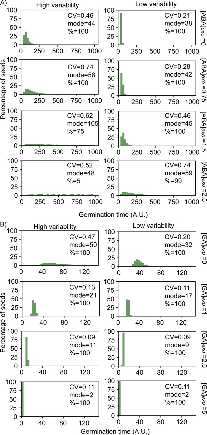
Simulated germination time distributions for a range of concentrations of exogenous abscisic acid (ABA) and gibberellic acid (GA).
Simulation results of adding increasing concentrations of exogenous ABA (A) or GA (B), showing germination time distributions and the coefficient of variation (CV), mode and percentage germination for those distributions. Simulations were performed starting from a point in the parameter space that shows higher germination time variability (left) and lower germination time variability (right) when no exogenous ABA or GA is added. Results correspond to a subset of the same simulations from those presented in Figure 6 and Figure 6—figure supplement 1. See corresponding nullcline analyses for some of these panels in Figure 6—figure supplement 3.
Figure 6—figure supplement 3
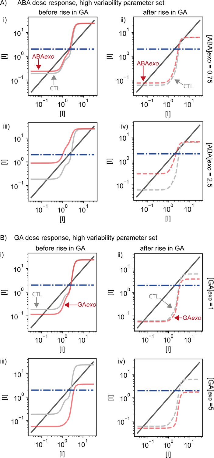
Results of nullcline analysis for abscisic acid (ABA) and gibberellic acid (GA) dose responses applied to the high variability parameter set.
Plots are for example cases from Figure 6 and Figure 6—figure supplement 1. (A) Examples of nullcline analyses for two doses of exogenous ABA. Left-hand panels (i and iii) show the cases at the beginning of the simulations prior to the rise in basal GA production. Right-hand panels (ii and iv) show plots for after the rise in basal GA production. Light grey solid (i and iii) and dashed (ii and iv) lines show the control simulations without exogenous addition of ABA and red solid (i and iii) and dashed (ii and iv) lines show the simulations with addition of exogenous ABA (the level added is indicated on the right). Steady-state solutions are shown by the intersections of the dark grey solid line with the light grey or red lines. Dashed blue line is the threshold below which Integrator must drop for germination to occur. Exogenous application of ABA can enhance the stability of the non-germination state (see Materials and methods), making it more difficult to switch to the germination state, driving a very long-tailed or flat distribution of germination times (Figure 6—figure supplement 2A). Exogenous ABA also shifts the low Integrator germination steady state higher, closer to the threshold for germination (compare the intersections of dashed red and dashed grey lines with the solid grey line). (B) As for (A), but for the addition of exogenous GA. Exogenous application of GA can destroy bistability before and after the rise of GA production, making the germination steady state the only possible steady state. This allows seeds to germinate earlier, with less variability (Figure 6—figure supplement 2B).
Figure 6—figure supplement 4
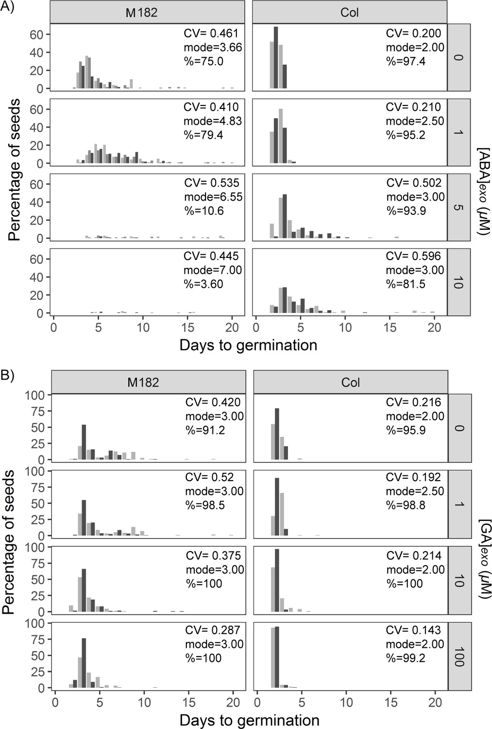
Effects of abscisic acid (ABA) and gibberellic acid (GA) on germination time distributions for example high and low variability lines.
(A) Effect of increasing exogenous ABA concentration on the distribution of germination times for the high variability MAGIC line, M182 (left panels), and the low variability accession, Col-0 (right panels). Plots show the percentage of all seeds that were sown, which germinated on a given day. Horizontal rows of panels show increasing concentrations of ABA (see labels on the right). Shades of grey indicate experimental replicates (at least two for each genotype). (B) As for (A), but for exogenous GA. Figure 6—figure supplement 4—source data 1 contains source data for (A) and (B).
-
Figure 6—figure supplement 4—source data 1
Figure6_FigureSupplement4_ColM182_ABA_GA.
- https://cdn.elifesciences.org/articles/59485/elife-59485-fig6-figsupp4-data1-v1.tds
Figure 7
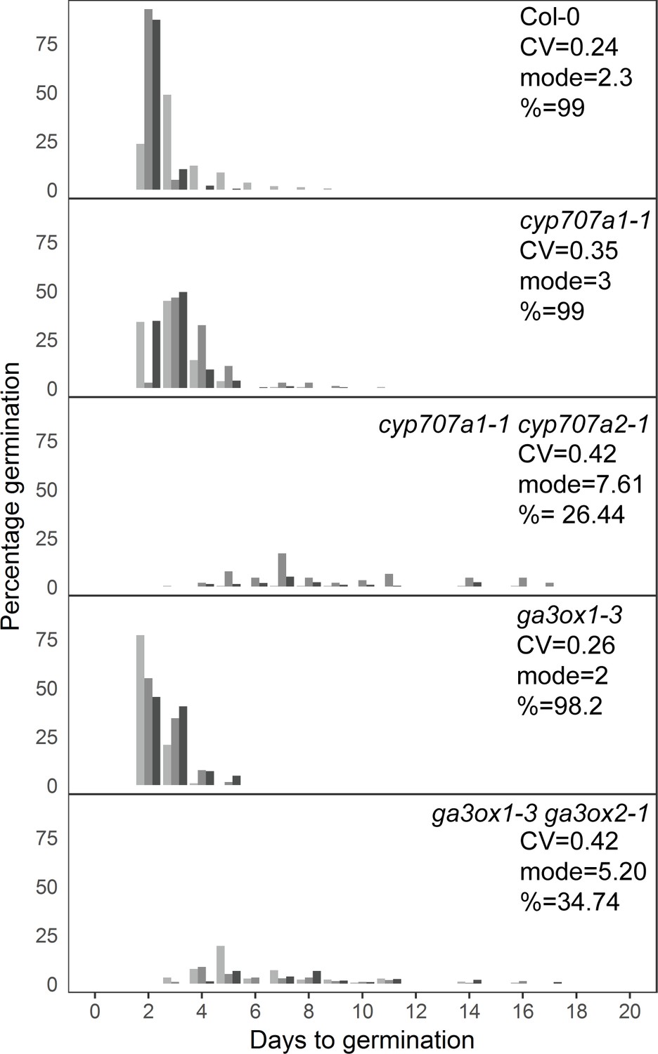
Mutants with altered levels of abscisic acid (ABA) and gibberellic acid (GA) have altered germination time variability.
Distributions of germination times for indicated genotypes. cyp707a1-1 and cyp707a1-1 cyp707a2-1 mutants lack enzymes involved in ABA catabolism, while ga3ox-3 and ga3ox1-3 ga3ox2-1 mutants lack enzymes involved in GA biosynthesis. Plots show the percentage of all seeds that were sown, that germinated on a given day. Grey-coloured bars show the germination time distribution of seed batches from replicate mother plants. For Col-0 and each mutant, the mean coefficient of variation of germination times, mode days to germination and final percentage germination is shown (averaged across the replicate batches [n = 3]). Data are representative of at least two independent experiments for each genotype. Source data is provided in Figure 7—source data 1.
-
Figure 7—source data 1
Figure7_MutantsGerm.
- https://cdn.elifesciences.org/articles/59485/elife-59485-fig7-data1-v1.tds
Author response image 1

Tables
Table 1
High and low variability lines used for abscisic acid (ABA) and gibberellic acid (GA) dose responses and their haplotypes at the Chr3 and Chr5 quantitative trait loci .
Haplotypes were classified according to their estimated effect on coefficient of variation (CV), as shown in Figure 4—figure supplement 2. Haplotype effect is classified as low/high when its average predicted effect is less than/higher than the mean haplotype effect, and the 95% confidence interval of the haplotype's effect does not overlap with mean haplotype effect. Haplotype effect is classified as medium when its 95% confidence interval overlaps with mean haplotype effect.
| Line | H/L variability | Chr3 haplotype | Chr3 haplotype effect on CV | Chr5 haplotype | Chr5 haplotype effect on CV | |
|---|---|---|---|---|---|---|
| 143 | High | Can | Medium | Zu | High | |
| 178 | High | Wu | High | Rsch | Medium | |
| 182 | High | Edi | Medium | Hi | Medium | |
| 285 | High | Ler | High | Zu | High | |
| 393 | High | Ler | High | Kn | High | |
| 53 | High | Sf | High | Rsch | Medium | |
| 108 | Low | Tsu | Low | Rsch | Medium | |
| 123 | Low | Bur | Medium | Wu | Medium | |
| 151 | Low | Bur | Medium | Wu | Medium | |
| 213 | Low | Wil | Low | Can | Medium | |
| 467 | Low | Wil | Low | Edi | Low | |
| Col-0 | Low | Col-0 | Low | Col-0 | Medium |
Key resources table
| Reagent type (species) or resource | Designation | Source or reference | Identifiers | Additional information |
|---|---|---|---|---|
| Biological samples (Arabidopsis thaliana) | MAGIC lines | NASC | NASC ID: N782242 | PMID:19593375 |
| Biological samples (Arabidopsis thaliana) | MAGIC parental accessions | NASC | IDs of individual parental accessions: http://arabidopsis.info/CollectionInfo?id=112 | PMID:19593375 |
| Biological samples (Arabidopsis thaliana) | Spanish accessions | NASC | PMID:26991665 | |
| Biological sample (Arabidopsis thaliana) | cyp707a1-1 | PMID:16543410 | Eiji Nambara, University of Toronto | |
| Biological sample (Arabidopsis thaliana) | cyp707a1-1 cyp707a2-1 | PMID:16543410 | Eiji Nambara, University of Toronto | |
| Biological sample (Arabidopsis thaliana) | ga3ox1-3 | NASC | NASC ID: N6943 | PMID:16460513 |
| Biological sample (Arabidopsis thaliana) | ga3ox1-3 ga3ox2-1 | NASC | NASC ID: N6944 | PMID:16460513 |
| Biological sample (Arabidopsis thaliana) | dog1-3 (Col-0) (SALK 000867) | NASC | NASC ID: N500867 | PMID:17065317 |
| Biological sample (Arabidopsis thaliana) | anac060 (SALK 012554C) | NASC | NASC ID: N665285 | PMID:24625790 |
| Biological sample (Arabidopsis thaliana) | ahg1-5 | PMID:28706187 | Guillaume Née, University of Münster | |
| Biological sample (Arabidopsis thaliana) | dog1 (No-0) (dog1 mutant in No-0 background) | RIKEN | BRC number: pst21966 Line number: 15-3980-1 | |
| Sequence-based reagent | DOG1N_F | This paper | PCR primers | GAAATCCGCTCCTTGTACCG See Supplementary file 4 |
| Sequence-based reagent | DOG1N_R | This paper | PCR primers | GCATCCCTGAGCTCAAACAA See Supplementary file 4 |
| Sequence-based reagent | Ds5-2a | PMID:14996221 | PCR primers | TCCGTTCCGTTTTCGTTTTTTAC See Supplementary file 4 |
| Sequence-based reagent | DOG1-3 F | This paper | PCR primers | TTCCAGGAACGTTGTCGTATC See Supplementary file 4 |
| Sequence-based reagent | DOG1-3 R | This paper | PCR primers | AGTTTGTGACCCACACAAAGC See Supplementary file 4 |
| Sequence-based reagent | LBb1.3 | http://signal.salk.edu/tdnaprimers.2.html | PCR primers | ATTTTGCCGATTTCGAAC See Supplementary file 4 |
| Sequence-based reagent | ANAC060 F | This paper | PCR primers | TGGACTCTGTTTGAAGCCTTG See Supplementary file 4 |
| Sequence-based reagent | ANAC060 R | This paper | PCR primers | TATGCCTGTCCTGATTTGCTC See Supplementary file 4 |
| Sequence-based reagent | AHG1 LP | PMID:28706187 | PCR primers | ACCGACACGTGTTCTGTCTTC See Supplementary file 4 |
| Sequence-based reagent | AHG1 RP | PMID:28706187 | PCR primers | CTAAAACTCGACCACCAGCTG See Supplementary file 4 |
| Chemical compound, drug | Gibberellin A4 | Sigma Aldrich | G7276 | |
| Chemical compound, drug | Abscisic acid | Sigma Aldrich | A1049 | |
| Commercial assay, kit | NEB Next Ultra DNA Library Prep Kit | New England BioLabs | E7370L | |
| Software, algorithm | Organism | PMID:15961462 | https://gitlab.com/slcu/teamHJ/Organism | |
| Software, algorithm | R | R Foundation for Statistical Computing | https://www.R-project.org/ | |
| Software, algorithm | Python | Python Software Foundation | Version: Python 2.7 https://www.python.org/download/releases/2.7/ | |
| Software, algorithm | Data analysis and modelling scripts | This paper | https://gitlab.com/slcu/teamJL/abley_formosa_etal_2020 ; Abley et al., 2021 copy archived at swh:1:rev:0a97b841e58b128c174d93fc759b28f1df2966a2 |
Table 2
Default values for each parameter in our mathematical model and varying parameters used in figures showing 1D parameter scans.
βX: production rate for X; vX: degradation rate for X; θX,Y: threshold above which Y has an effect on X; CX,Y: coefficient for regulatory functions of Y acting on X; h: exponent of regulatory functions; V: effective system volume (modulates noise). All parameter units are arbitrary.
| Default | Figure 5B–D | Figure 5—figure supplement 2A | Figure 5—figure supplement 2B | Figure 5—figure supplement 2C | Figure 5—figure supplement 2D | |
|---|---|---|---|---|---|---|
| βABA | 1 | Varying | ||||
| βGA | 0.3 | |||||
| βGA,Z | 0.01 | |||||
| βZ | 39 | |||||
| βI | 0.3 | |||||
| vABA | 1 | 1.58 | ||||
| vGA | 1 | |||||
| vZ | 0.1 | |||||
| vI | 0.4 | |||||
| θABA,I | 3.7 | |||||
| θGA,I | 1.2 | |||||
| θI,ABA | 6.5 | Varying | 10 | 10 | ||
| θI,GA | 6 | Varying | Varying | |||
| CABA,I | 10 | |||||
| CGA,I | 4 | |||||
| CI,ABA | 10 | |||||
| CI,GA | 6 | |||||
| h | 4 | |||||
| V | 30 | 100 | Varying |
Additional files
-
Supplementary file 1
Supplementary_File1_MAGICs.
- https://cdn.elifesciences.org/articles/59485/elife-59485-supp1-v1.csv
-
Supplementary file 2
Supplementary_File2_MAGICParents.
- https://cdn.elifesciences.org/articles/59485/elife-59485-supp2-v1.csv
-
Supplementary file 3
Supplementary_File3_SpanishAccessions.
- https://cdn.elifesciences.org/articles/59485/elife-59485-supp3-v1.csv
-
Supplementary file 4
Genotyping primers.
- https://cdn.elifesciences.org/articles/59485/elife-59485-supp4-v1.xlsx
-
Transparent reporting form
- https://cdn.elifesciences.org/articles/59485/elife-59485-transrepform-v1.docx
Download links
A two-part list of links to download the article, or parts of the article, in various formats.
Downloads (link to download the article as PDF)
Open citations (links to open the citations from this article in various online reference manager services)
Cite this article (links to download the citations from this article in formats compatible with various reference manager tools)
An ABA-GA bistable switch can account for natural variation in the variability of Arabidopsis seed germination time
eLife 10:e59485.
https://doi.org/10.7554/eLife.59485


