On the objectivity, reliability, and validity of deep learning enabled bioimage analyses
- Institute of Clinical Neurobiology, University Hospital Würzburg, Germany
- Department of Business and Economics, University of Würzburg, Germany
- Institute of Physiology I, Westfälische Wilhlems-Universität, Germany
- Department of Pharmacology, Medical University of Innsbruck, Austria
- Department of Pharmacology and Toxicology, Institute of Pharmacy and Center for Molecular Biosciences Innsbruck, University of Innsbruck, Austria
- Department of Child and Adolescent Psychiatry, Center of Mental Health, University Hospital Würzburg, Germany
- Comprehensive Anxiety Center, Germany
Figures
Figure 1 with 2 supplements
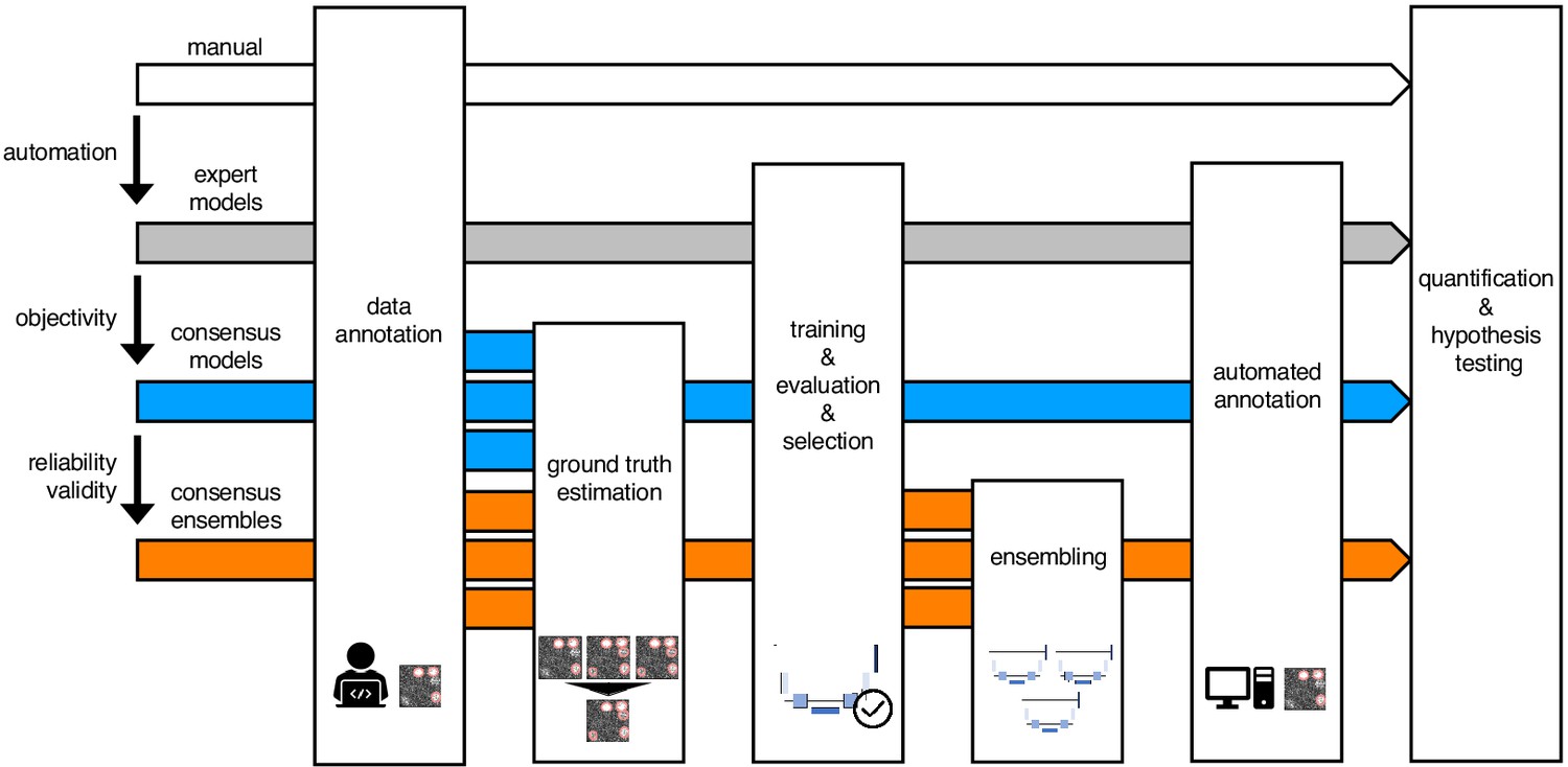
Schematic illustration of bioimage analysis strategies and corresponding hypotheses.
Four bioimage analysis strategies are depicted. Manual (white) refers to manual, heuristic fluorescent feature annotation by a human expert. The three DL-based strategies for automatized fluorescent feature annotation are based on expert models (gray), consensus models (blue) and consensus ensembles (orange). For all DL-based strategies, a representative subset of microscopy images is annotated by human experts. Here, we depict labels of cFOS-positive nuclei and the corresponding annotations (pink). These annotations are used in either individual training datasets (gray: expert models) or pooled in a single training dataset by means of ground truth estimation from the expert annotations (blue: consensus models, orange: consensus ensembles). Next, deep learning models are trained on the training dataset and evaluated on a holdout validation dataset. Subsequently, the predictions of individual models (gray and blue) or model ensembles (orange) are used to compute binary segmentation masks for the entire bioimage dataset. Based on these fluorescent feature segmentations, quantification and statistical analyses are performed. The expert model strategy enables the automation of a manual analysis. To mitigate the bias from subjective feature annotations in the expert model strategy, we introduce the consensus model strategy. Finally, the consensus ensembles alleviate the random effects in the training procedure and seek to ensure reliability and eventually, validity.
Figure 1—figure supplement 1
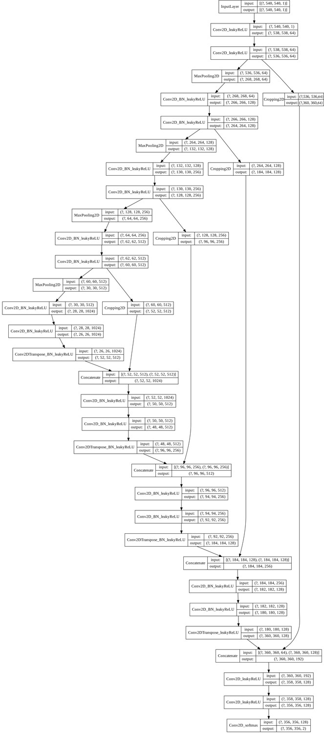
U-Net architecture.
The U-Net architecture was adapted from Falk et al., 2019. The input and output shapes denote (minibatch size x height x width x channels), where the mini-batch size is not specified. If applicable, the names of the layers describe the containing operations (e.g.: Conv2D_BN_leakyReLU represents a 2D convolution followed by a batch normalization layer and a leakyReLu activation function). All convolutional layers were instantiated with a kernel size of 3 × 3, a stride of one and, no padding, except for the last convolution (1 × 1 kernel). The leaky ReLU has a leakage factor of 0.1 and the max-pooling operation a stride of two. The up-convolution (Conv2DTranspose) has a kernel size of 2 × 2 and strides of two.
Figure 1—figure supplement 2
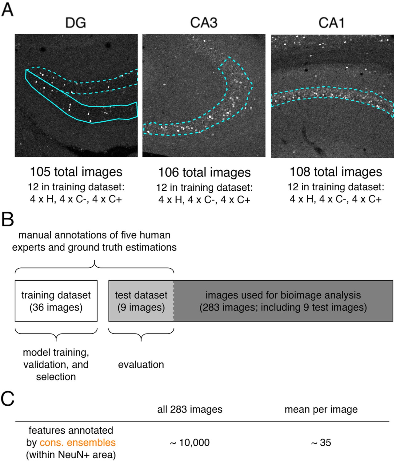
Illustration of bioimage dataset Lab-Wue1.
(A) A total of 319 images showing cFOS immunoreactivity in the dorsal hippocampus of mice was split up in 105 images of the Dentate gyrus, 106 images of CA3 and 108 images of CA1. To create a balanced training dataset, four images of each experimental condition were randomly selected (H, C-, C+) from each hippocampal subregion (DG, CA3, CA1; 4 × 3 × 3 = 36 images). (B) Five expert neuroscientists (experts 1–5) manually annotated cFOS-positive nuclei in the selected 36 images of the training dataset and in nine additional images (test dataset). The test images represented one image per region and condition (3 × 3). Annotation was performed independently and on different computers and screens. The training dataset was used to train either expert specific models (only annotations of a single expert were used) or consensus models (est. GT annotations computed from the annotations of all five experts were used). Using k-fold cross-validation during the training, we were able to test the model performance and to ultimately select only those models that reached human level performance. The final evaluation of all models was then performed on the additional nine images of the test dataset. For bioimage analyses, we used the remaining 274 images and the nine test images. (C) On average, each consensus ensemble annotated ∼10,000 cFOS-positive feature within the NeuN-positive areas in all 283 images used for bioimage analysis, which is equivalent to ∼35 features per image.
Figure 2 with 4 supplements
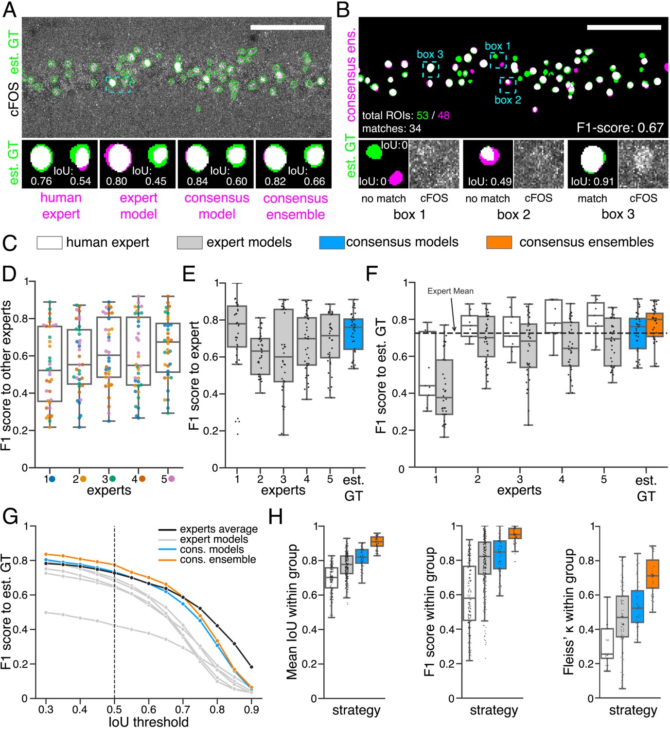
Similarity analysis of fluorescent feature annotations by manual or DL-based strategies.
(A) Representative example of IoU calculations on a field of view (FOV) in a bioimage. Image raw data show the labeling of cFOS in a maximum intensity projection image of the CA1 region in the hippocampus (brightness and contrast enhanced). The similarity of estimated ground truth (est. GT) annotations (green), derived from the annotations of five expert neuroscientists, are compared to those of one human expert, an expert model, a consensus model, and a consensus ensemble (magenta, respectively). IoU results of two ROIs are shown in detail for each comparison (magnification of cyan box). Scale bar: 100 µm. (B) F1 score calculations on the same FOV as shown in (A). The est. GT annotations (green; 53 ROIs) are compared to those of a consensus ensemble (magenta; 48 ROIs). IoU-based matching of ROIs at an IoU-threshold of is depicted in three magnified subregions of the image (cyan boxes 1-3). Scale bar: 100 µm. (C–H) All comparisons are performed exclusively on a separate image test set which was withheld from model training and validation. (C) Color coding refers to the individual strategies, as introduced in Figure 1: white: manual approach, gray: expert models, blue: consensus models, orange: consensus ensembles. (D) between individual manual expert annotations and their overall reliability of agreement given as the mean of Fleiss‘ . (E) between annotations predicted by individual models and the annotations of the respective expert (or est. GT), whose annotations were used for training. Nmodels per expert = 4. (F) between manual expert annotations, the respective expert models, consensus models, and consensus ensembles compared to the est. GT as reference. A horizontal line denotes human expert average. Nmodels = 4, Nensembles = 4. (G) Means of of the individual DL-based strategies and of the human expert average compared to the est. GT plotted for different IoU matching thresholds t. A dashed line indicates the default threshold . Nmodels = 4, Nensembles = 4. (H) Annotation reliability of the individual strategies assessed as the similarities between annotations within the respective strategy. We calculated , and Fleiss‘ . Nexperts = 5, Nmodels = 4, Nensembles = 4.
Figure 2—figure supplement 1
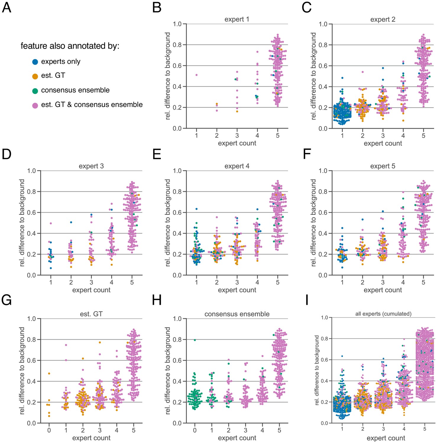
Extended subjectivity analysis.
The subjectivity analysis depicts the relationship between the relative intensity difference of a florescent feature (ROI) to the background and the annotation count of human experts. A visual interpretation indicates that the annotation probability of a ROI is positively correlated with its relative relative intensity. The relative intensity difference is calculated as , where is the mean signal intensity of the ROI and the mean signal intensity of its nearby outer area. We considered matching ROIs at an IoU threshold of . The expert in the title of the respective plot was used to create the region proposals of the ROIs, that is, the annotations served as origin for the other pairwise comparisons. (A) Legend of color codes: blue depicts that a ROI was only annotated by one or more human experts; yellow depicts the ROIs that were present in the estimated ground truth; green shows the ROIs that are only present in an exemplary consensus ensemble; pink depicts ROIs that are present in both estimated ground truth and consensus ensemble (B–I) All calculations are performed on the test set (n = 9 images) which was withheld from model training and validation. (B–F) The individual expert analysis shows the effects of different heuristic evaluation criteria. (G) The analysis of the est. GT annotations reveals the limitations of the ground truth estimation algorithm, which is based on the human annotations. An expert count of zero can result from merging different ROIs. (H) The analysis of a representative consensus ensemble shows that human annotators may have missed several ROIs (green) even with a large relative difference to the background. (I) Cumulative summary of B-F.
Figure 2—figure supplement 2
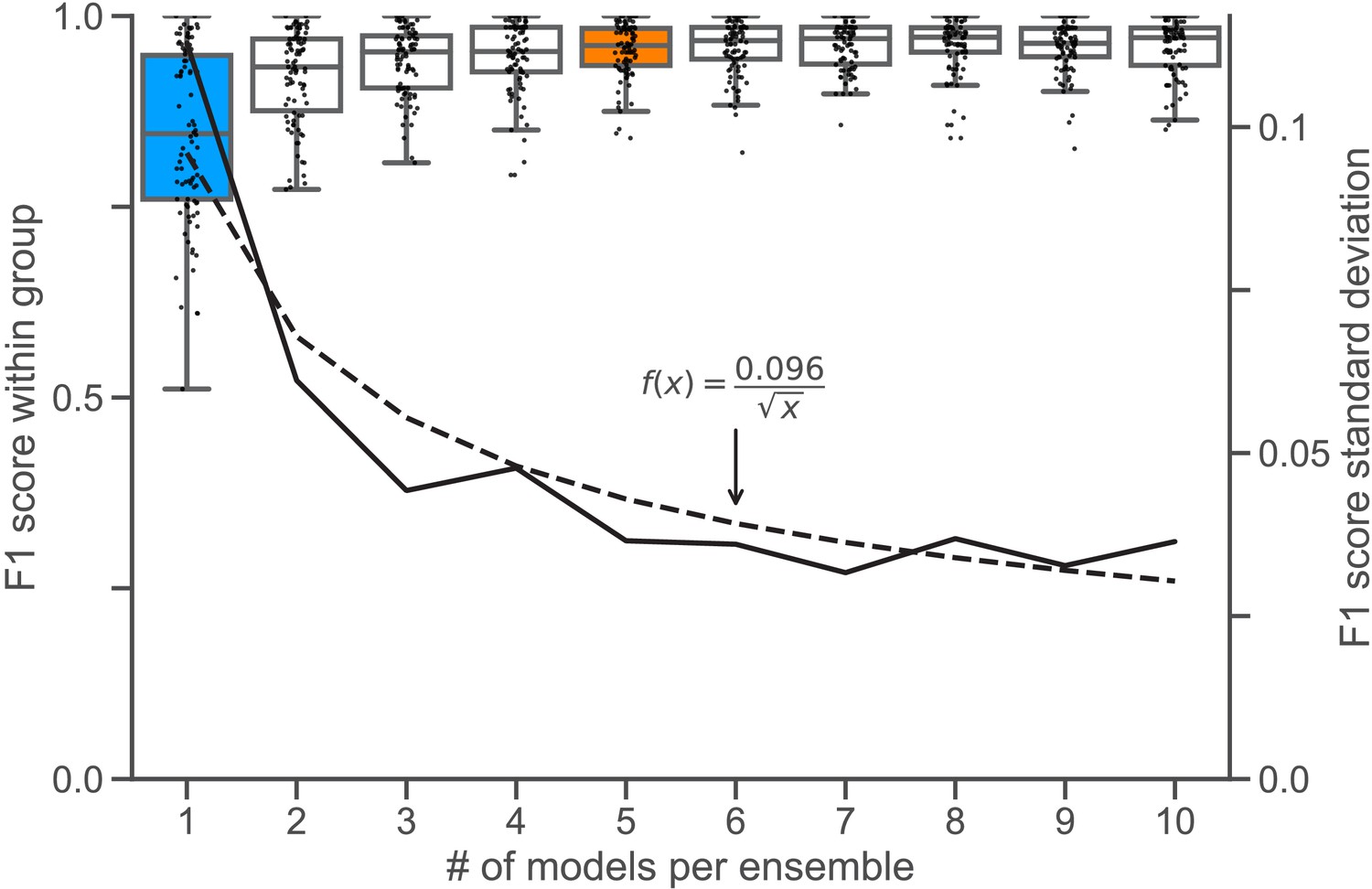
Ensemble size and reliability.
To determine an appropriate size for the consensus ensembles, we analyzed the homogeneity of the results through a similarity analysis. Therefore, we calculated the at an IoU matching threshold of for each ensemble size on the holdout test set (n = 9 images). Stratified on the cross validation splits, we randomly sampled the ensembles from a collection of trained consensus models. We repeated this procedure five times to mitigate the random effect of the ensemble composition (Nensembles = 5 for each i). The blue box () depicts the variability between different consensus models. The orange box () shows the variability of the finally chosen size for the consensus ensembles, as no substantial reduction in variation can be observed for larger i. In addition, corresponds to the number of cross validation splits (), meaning that the ensembles have seen the entire training set. The black line denotes the standard deviation of , which is scaled at the right y-Axis. The dashed black line denotes the best fitting function of type with for the standard deviation.
Figure 2—figure supplement 3
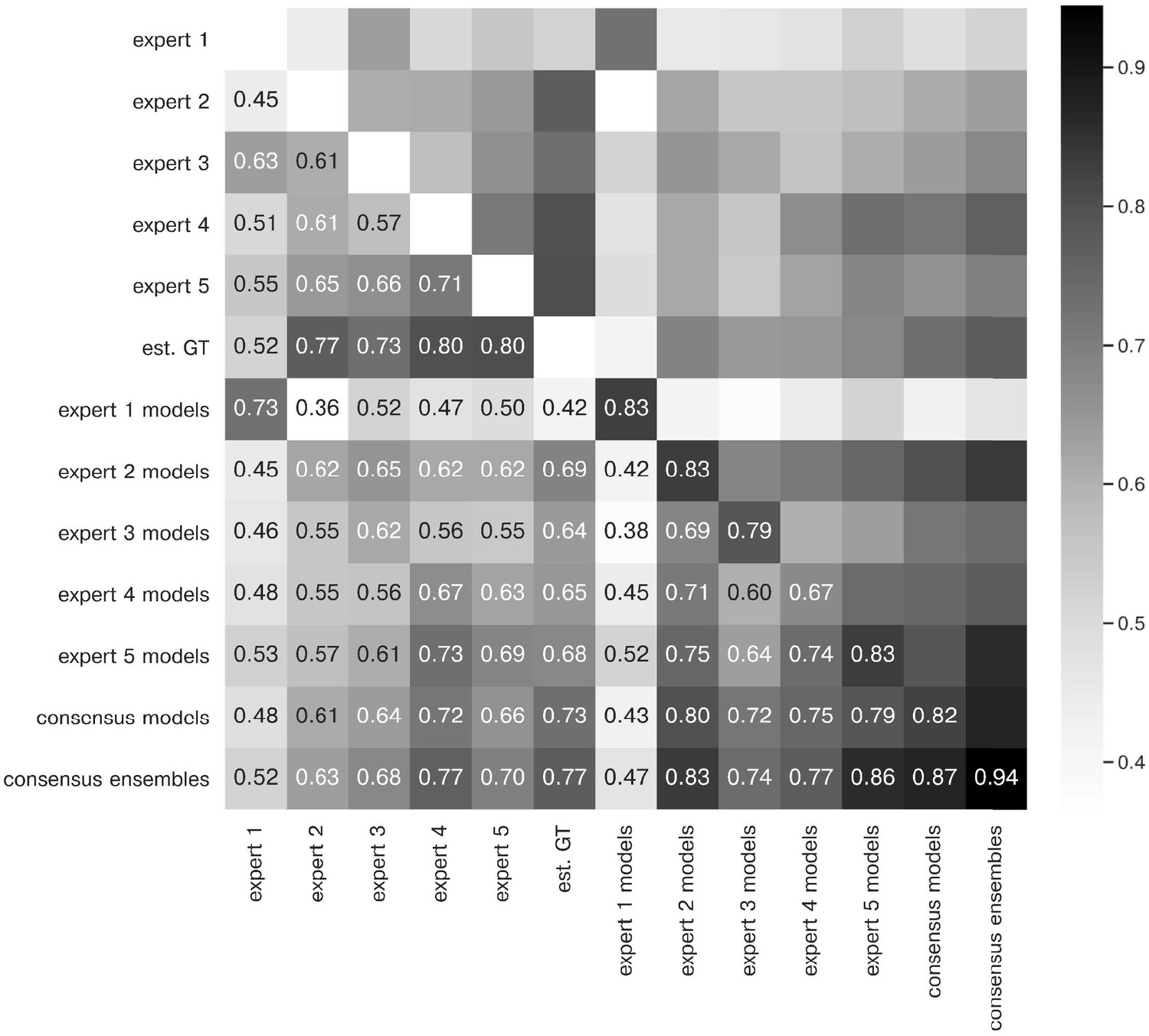
Extended similarity analysis: F1 score.
The heatmap shows the mean of at a matching IoU-threshold of for the image feature annotations of the indicated experts. Segmentation masks of the five human experts (Nexpert = 1 per expert), the estimated ground-truth (Nest. GT = 1), the respective expert models, the consensus models, and the consensus ensembles (Nmodels = 4 per model or ensemble) are compared. The diagonal values show the inter-model reliability (no data available for the human experts who only annotated the images once). The consensus ensembles show the highest reliability (0.94) and perform on par with human experts compared to the est. GT (0.77). Both expert 1 and the corresponding expert 1 models show overall low similarities to other experts and expert models, while sharing a high similarity to each other (0.73).
Figure 2—figure supplement 4
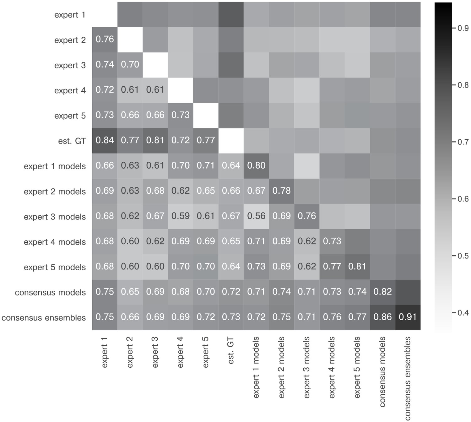
Extended similarity analysis: mean IoU.
The heatmap shows the mean of for the image feature annotations of the indicated experts. Segmentation masks of the five human experts (Nexpert = 1 per expert), the estimated ground-truth (Nest. GT = 1), the respective expert models, the consensus models, and the consensus ensembles (Nmodels = 4 per model or ensemble) are compared. The diagonal values show the inter-model reliability (no data available for the human experts who only annotated the images once). Again, consensus ensembles show highest reliability (0.91). Est. GT annotations are directly derived from manual expert annotations, which renders this comparison favorable.
Figure 3 with 1 supplement
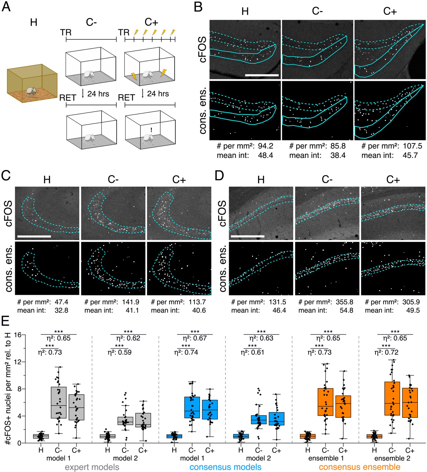
Application of different DL-based strategies for fluorescent feature annotation.
The figure introduces how three DL-based strategies are applied for annotation of a representative fluorescent label, here cFOS, in a representative image data set. Raw image data show behavior-related changes in the abundance and distribution of the protein cFOS in the dorsal hippocampus, a brain center for encoding of context-dependent memory. (A) Three experimental groups were investigated: Mice kept in their homecage (H), mice that were trained to a context, but did not experience an electric foot shock (C-) and mice exposed to five foot shocks in the training context (C+). 24 hr after the initial training (TR), mice were re-exposed to the training context for memory retrieval (RET). Memory retrieval induces changes in cFOS levels. (B–D) Brightness and contrast enhanced maximum intensity projections showing cFOS fluorescent labels of the three experimental groups (H, C-, C+) with representative annotations of a consensus ensemble, for each hippocampal subregion. The annotations are used to quantify the number of cFOS-positive nuclei for each image (#) per mm2 and their mean signal intensity (mean int., in bit-values) within the corresponding image region of interest, here the neuronal layers in the hippocampus (outlined in cyan). In B: granule cell layer (supra- and infrapyramidal blade), dotted line: suprapyramidal blade, solid line: infrapyramidal blade. In C: pyramidal cell layer of CA3; in D: pyramidal cell layer in CA1. Scale bars: 200 µm. (E) Analyses of cFOS-positive nuclei per mm2, representatively shown for stratum pyramidale of CA1. Corresponding effect sizes are given as for each pairwise comparison. Two quantification results are shown for each strategy and were selected to represent the lowest (model 1 or ensemble 1) and highest (model 2 or ensemble 2) effect sizes (increase in cFOS) reported within each annotation strategy. Total analyses performed: Nexpert models = 20, Nconsensus models = 36, Nconsensus ensembles = 9. Number of analyzed mice (N) and images (n) per experimental condition: NH = 7, NC- = 7, NC+ = 6; nH = 36, nC- = 32, nC+ = 28. ***p<0.001 with Mann-Whitney-U test. Statistical data are available in Figure 3—source data 1.
-
Figure 3—source data 1
Source files for analyses of cFOS-positive nuclei in CA1.
- https://cdn.elifesciences.org/articles/59780/elife-59780-fig3-data1-v2.zip
Figure 3—figure supplement 1
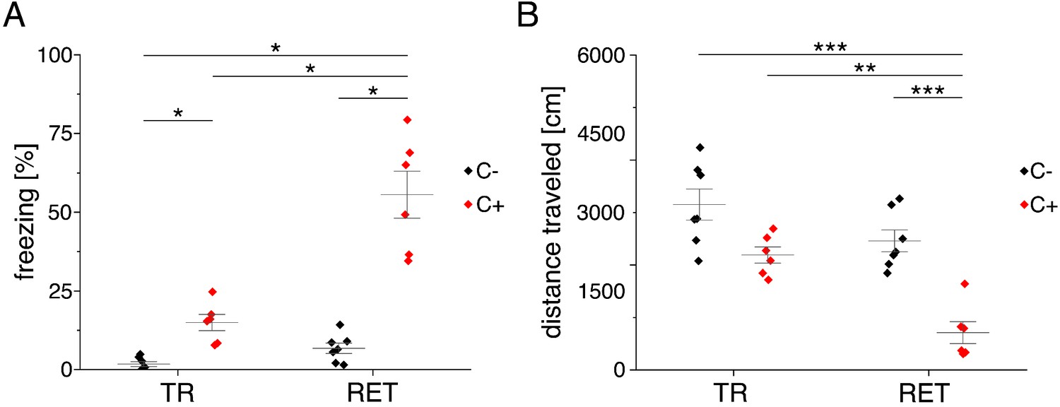
Behavioral analysis Lab-Wue1.
(A) Fear acquisition was observed in conditioned mice (C+), while unconditioned controls (C-) did not show freezing behavior during initial context exposure (TR). In the memory retrieval session (RET), conditioned mice showed strong freezing behavior, while unconditioned mice did not freeze in response to the training context (X2(3) = 20.894, p<0.001, NTR C- = 7, NTR C+ = 6, NRET C- = 7, NRET C+ = 6, Kruskal-Wallis ANOVA followed by pairwise Mann-Whitney tests with Bonferroni correction, *p<0.05). (B) Distance traveled in the training context is reduced in fear conditioned mice (F(3, 22) = 19.484, p<0.001, NTR C- = 7, NTR C+ = 6, NRET C- = 7, NRET C+ = 6, one-way ANOVA followed by pairwise t-tests with Bonferroni correction, **p<0.01, ***p<0.001). Source data is available as Figure 3—figure supplement 1—source data 1.
-
Figure 3—figure supplement 1—source data 1
Source files for behavioral analysis in Figure 3—figure supplement 1.
- https://cdn.elifesciences.org/articles/59780/elife-59780-fig3-figsupp1-data1-v2.zip
Figure 4
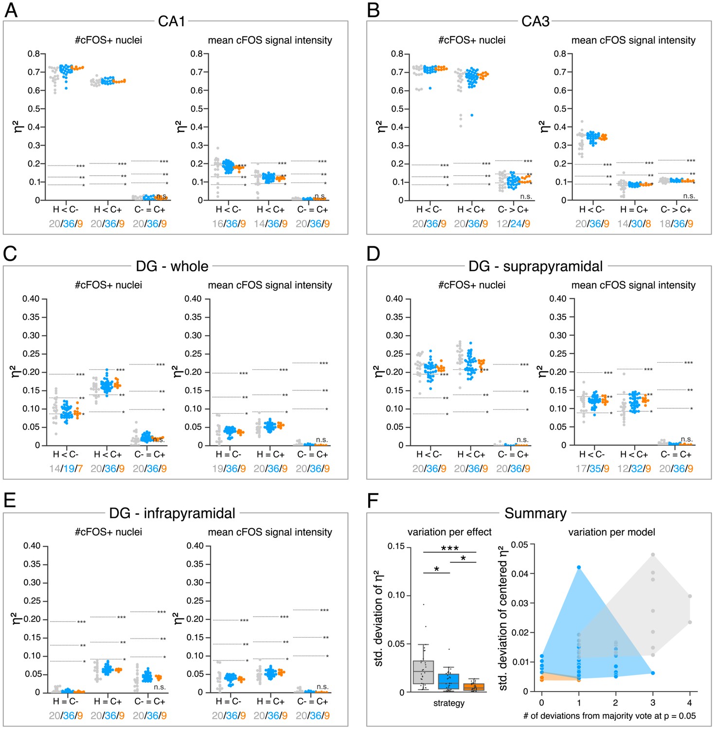
Consensus ensembles significantly increase reliability of bioimage analysis results.
(A–E) Single data points represent the calculated effect sizes for each pairwise comparison of all individual bioimage analyses for each DL-based strategy (gray: expert models, blue: consensus models, orange: consensus ensembles) in indicated hippocampal subregions. Three horizontal lines separate four significance intervals (n.s.: not significant, *: 0.05 ≥ p>0.01, **: 0.01 ≥ p>0.001, ***: p ≤ 0.001 after Bonferroni correction for multiple comparisons). The quantity of analyses of each strategy that report the respective statistical result of the indicated pairwise comparison (effect, x-axis) at a level of p ≤ 0.05 are given below each pairwise comparison in the corresponding color coding. In total, we performed all analyses with: Nexpert models = 20, Nconsensus models = 36, Nconsensus ensembles = 9. Number of analyzed mice (N) for all analyzed subregions: NH = 7, NC- = 7, NC+ = 6. Numbers of analyzed images (n) are given for each analyzed subregion. Source files including source data and statistical data are available in Figure 4—source data 1. (A) Analyses of cFOS-positive nuclei in stratum pyramidale of CA1. nH = 36, nC- = 32, nC+ = 28. (B) Analyses of cFOS-positive nuclei in stratum pyramidale of CA3. nH = 35, nC- = 31, nC+ = 28. (C) Analyses of cFOS-positive nuclei in the granule cell layer of the whole DG. nH = 35, nC- = 31, nC+ = 27. (D) Analyses of cFOS-positive nuclei in the granule cell layer of the suprapyramidal blade of the DG. nH = 35, nC- = 31, nC+ = 27. (E) Analyses of cFOS-positive nuclei in the granule cell layer of the infrapyramidal blade of the DG. nH = 35, nC- = 31, nC+ = 27. (F) Reliability of bioimage analysis results are assessed as variation per effect (left side) and variation per model (right side). For the variation per effect, single data points represent the standard deviation of reported effect sizes (), calculated within each DL-based strategy for each of the 30 pairwise comparisons. Consensus ensembles show significantly lower standard (std.) deviations of per pairwise comparison compared to alternative strategies (X2(2) = 26.472, p<0.001, Neffects = 30, Kruskal-Wallis ANOVA followed by pairwise Mann-Whitney tests with Bonferroni correction, *p<0.05, ***p<0.001). For the variation per model, the standard deviation of centered across all pairwise comparisons was calculated for each individual model and ensemble (y-axis). In addition, the number of deviations from the congruent majority vote (at p ≤ 0.05 after Bonferroni correction for multiple comparisons) were determined for each individual model and ensemble across all pairwise comparisons (x-axis). Visualizing the interaction of both measures for each model or model ensemble individually reveals that consensus ensembles show the highest reliability of all three DL-based strategies. The statistical data for the for variation per effect is available in Figure 4—source data 2.
-
Figure 4—source data 1
Source files for the analysis of cFOS positive nuclei in the hippocampal subregions.
- https://cdn.elifesciences.org/articles/59780/elife-59780-fig4-data1-v2.zip
-
Figure 4—source data 2
Statistical data for the variation per effect.
- https://cdn.elifesciences.org/articles/59780/elife-59780-fig4-data2-v2.zip
Figure 5 with 5 supplements
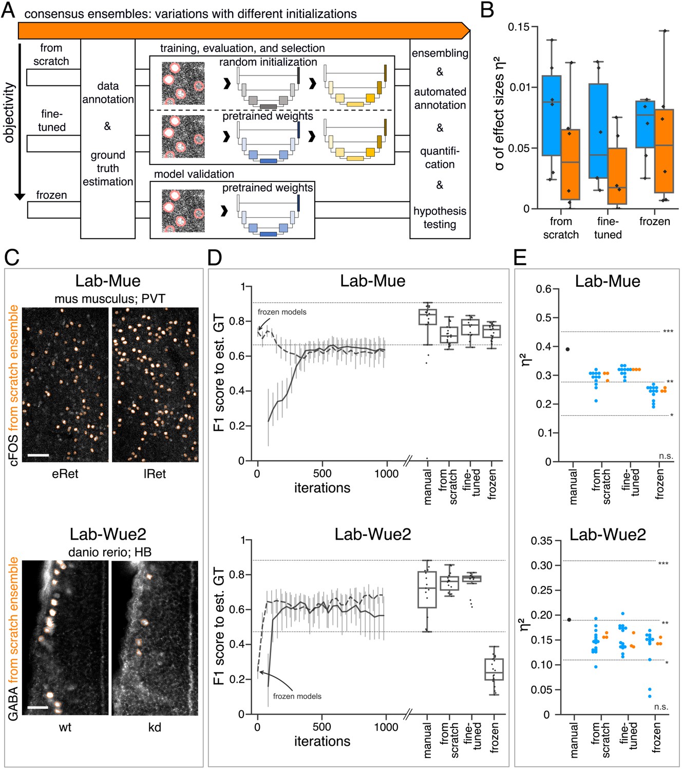
Consensus ensembles for DL-based feature annotation in external bioimage data sets.
(A) Schematic overview depicting three initialization variants for creating consensus ensembles on new datasets. Data annotation by multiple human experts and subsequent ground truth estimation are required for all three initialization variants. In the from scratch variant, a U-Net model with random initialized weights is trained on pairs of microscopy images and estimated ground truth annotations. This variant was used to create consensus ensembles for the initial Lab-Wue1 dataset. Alternatively, the same training dataset can be used to adapt a U-Net model with pretrained weights by means of transfer-learning (fine-tuned). In both variants, models are evaluated and selected on base of a validation set after model training. In a third variant, U-Net models with pretrained weights can be evaluated directly on a validation dataset, without further training (frozen). In all three variants, consensus ensembles of the respective models are then used for bioimage analysis. (B) Overall reliability of bioimage analysis results of each variant assessed as variation per effect. In all three strategies, consensus ensembles (orange) showed lower standard deviations than consensus models (blue). The frozen results need to be considered with caution as they are based on models that did not meet the selection criterion (see Figure 5—source data 3). Npairwise comparisons = 6; Nconsensus models = 15, and Nconsensus ensembles = 3 for each variant. (C–E) Detailed comparison of the two external datasets with highest (Lab-Mue) and lowest (Lab-Wue2) similarity to Lab-Wue1. (C) Representative microscopy images. Orange: representative annotations of a lab-specific from scratch consensus ensemble. PVT: para-ventricular nucleus of thalamus, eRet: early retrieval, lRet: late retrieval, HB: hindbrain, wt: wildtype, kd: gad1b knock-down. Scale bars: Lab-Mue 100 µm and Lab-Wue2 6 µm. (D) Mean of from scratch (solid line) and fine-tuned (dashed line) consensus models on the validation dataset over the course of training (iterations). Mean of frozen consensus models are indicated with arrows. Box plots show the among the annotations of human experts as reference and the mean of selected consensus models. Two dotted horizontal lines mark the whisker ends of the among the human expert annotations. (E) Effect sizes of all individual bioimage analyses (black: manual experts, blue: consensus models, orange: consensus ensembles). Three horizontal lines separate the significance intervals (n.s.: not significant, *: 0.05≥ p>0.01, **0.01≥ p>0.001, ***p ≤ 0.001 with Mann-Whitney-U tests). Lab-Mue: Nconsensus ensembles = 3 for all initialization variants; Nfrom scratch/fine-tuned consensus models = 12 (for each ensemble, 4/5 trained models per ensemble met the selection criterion), Nfrozen consensus models = 12 (for each ensemble, 4/4 models per ensemble did not meet the selection criterion). NeRet = 4, NlRet = 4; neRet = 12, nlRet = 11. Lab-Wue2: Nconsensus ensembles = 3 for each initialization variant; Nfrom scratch/fine-tuned consensus models = 15 (for each ensemble, 5/5 trained models per ensemble met the selection criterion), Nfrozen consensus models = 12 (for each ensemble, 4/4 models per ensemble did not meet the selection criterion). Nwt = 5, Nkd = 4, nwt = 20, nkd = 15. Source files of all statistical analyses (including Figure 5—figure supplement 2 and Figure 5—figure supplement 1) are available in Figure 5—source data 1. Information on all bioimage datasets (e.g. the number of images, image resolution, imaging techniques, etc.) are available in Figure 5—source data 2. Source files on model performance and selection are available in (Figure 5—source data 3).
-
Figure 5—source data 1
Statistical data for Lab-Mue, Lab-Wue2, Lab-Inns1, and Lab-Inns2.
- https://cdn.elifesciences.org/articles/59780/elife-59780-fig5-data1-v2.zip
-
Figure 5—source data 2
Characteristics of all five bioimage datasets.
- https://cdn.elifesciences.org/articles/59780/elife-59780-fig5-data2-v2.docx
-
Figure 5—source data 3
Model performance with selection criterion for Lab-Mue, Lab-Wue2, Lab-Inns1, and Lab-Inns2.
- https://cdn.elifesciences.org/articles/59780/elife-59780-fig5-data3-v2.zip
Figure 5—figure supplement 1
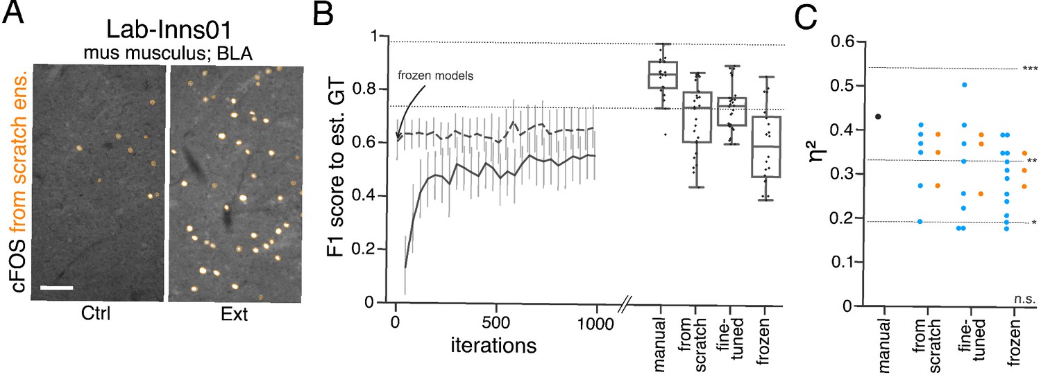
Performance of consensus ensembles on feature annotation in image dataset Lab-Inns01.
(A) Representative microscopy images. Orange: representative annotations of a lab-specific from scratch consensus ensemble. BLA: basolateral amygdala, Ctrl: control, Ext: extinction. Scale bar: 80 µm. (B) Mean of from scratch (solid line) and fine-tuned (dashed line) consensus models on the validation dataset over the course of training (iterations). Mean of frozen consensus models are indicated with an arrow. Box plots show the among the annotations of human experts as reference and the mean of selected consensus models. Two dotted horizontal lines mark the whisker ends of the among the human expert annotations. (C) Effect sizes of all individual bioimage analyses (black: manual experts, blue: consensus models, orange: consensus ensembles). Three horizontal lines separate four selected significance intervals (n.s.: not significant, *: 0.05 ≥ p>0.01, **: 0.01 ≥ p>0.001, ***: p ≤ 0.001). The analyses were performed with: Nconsensus ensembles = 3 for each initialization variant; Nfrom scratch consensus models = 6 (for each ensemble, 2/5 trained models per ensemble met the selection criterion), Nfine-tuned consensus models = 8 (for ensemble 1 and 2, 3/5 trained models per ensemble met the selection criterion; for ensemble 3, 2/5 trained models met the selection criterion), Nfrozen consensus models = 12 (for each ensemble, 4/4 models per ensemble did not meet the selection criterion). Thus, the frozen consensus model and ensemble results need to be considered with caution. NCtrl = 5, NExt = 5; nCtrl = 10, nExt = 9. Statistical data can be found in Figure 5—source data 1. Source files on model performance and selection are available in Figure 5—source data 3.
Figure 5—figure supplement 2
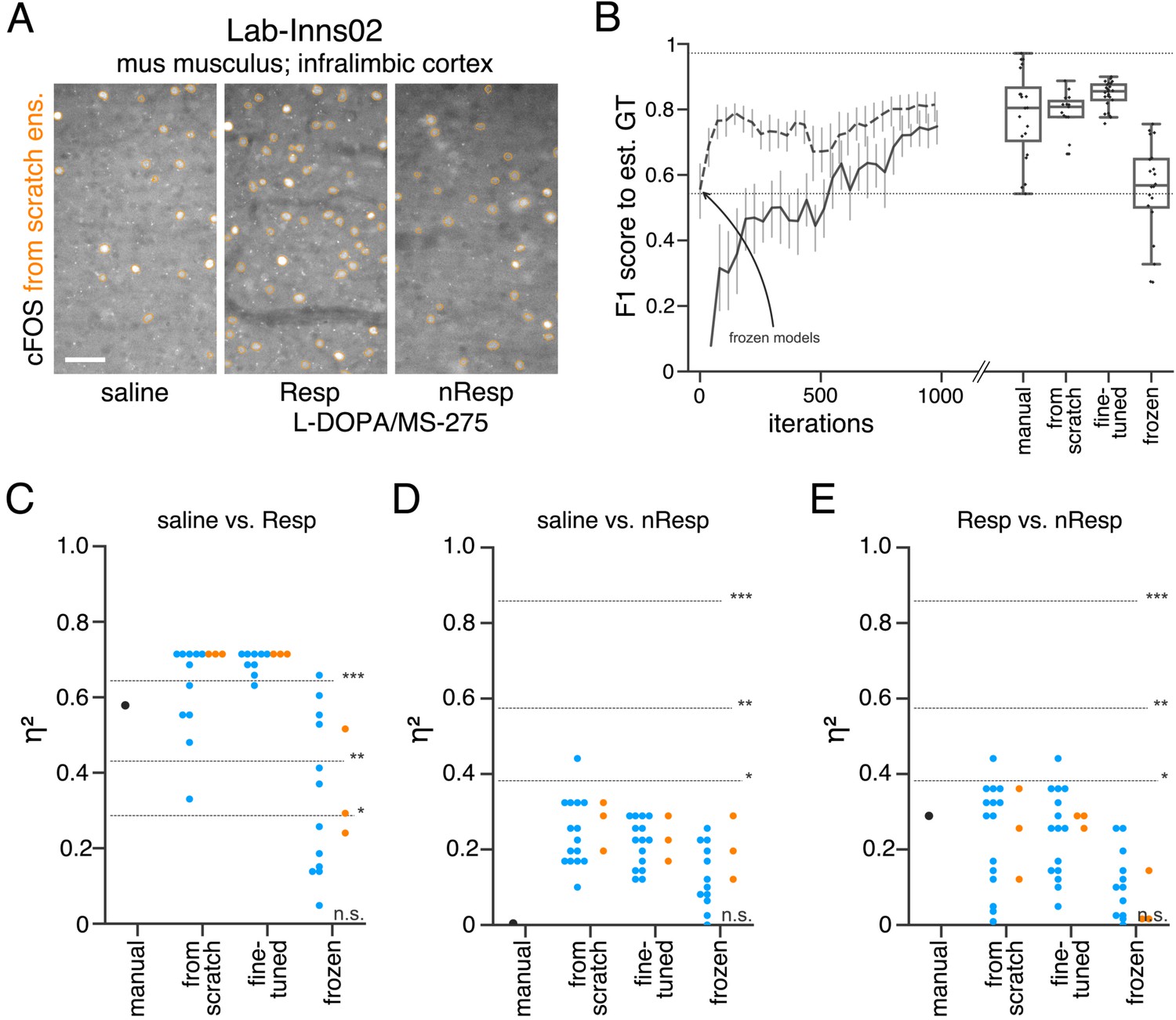
Performance of consensus ensembles on fluorescent feature annotation in image dataset Lab-Inns02.
(A) Representative microscopy images. Orange: representative annotations of a lab-specific from scratch consensus ensemble. Resp: responders, nResp: non-responders. Scale bar: 40 µm. (B) Mean of from scratch (solid line) and fine-tuned (dashed line) consensus models on the validation dataset over the course of training (iterations). Mean of frozen consensus models are indicated with an arrow. Box plots show the among the annotations of human experts as reference and the mean of selected consensus models. Two dotted horizontal lines mark the whisker ends of the among the human expert annotations. (C–E) Effect sizes of all individual bioimage analyses (black: manual experts, blue: consensus models, orange: consensus ensembles). Three horizontal lines separate four selected significance intervals (n.s.: not significant, *: 0.05 ≥ p>0.01, **: 0.01 ≥ p>0.001, ***: p ≤ 0.001 after Bonferroni correction for multiple comparisons). The analyses were performed with: Nconsensus ensembles = 3 for each initialization variant; Nfrom scratch consensus models = 15 (for each ensemble, 5/5 trained models per ensemble met the selection criterion), Nfine-tuned consensus models = 15, (for each ensemble, 5/5 trained models per ensemble met the selection criterion), Nfrozen consensus models = 12 (for each ensemble, 4/4 models per ensemble did not meet the selection criterion). Thus, the frozen consensus model and ensemble results need to be considered with caution. Nsaline = 6, NL-DOPA/MS-275 Resp = 6, NL-DOPA/MS-275 nResp = 3; nsaline = 10, nL-DOPA/MS-275 Resp = 10, nL-DOPA/MS-275 nResp = 5. Statistical data can be found in Figure 5—source data 1. Source files on model performance and selection are available in (Figure 5—source data 3).
Figure 5—figure supplement 3
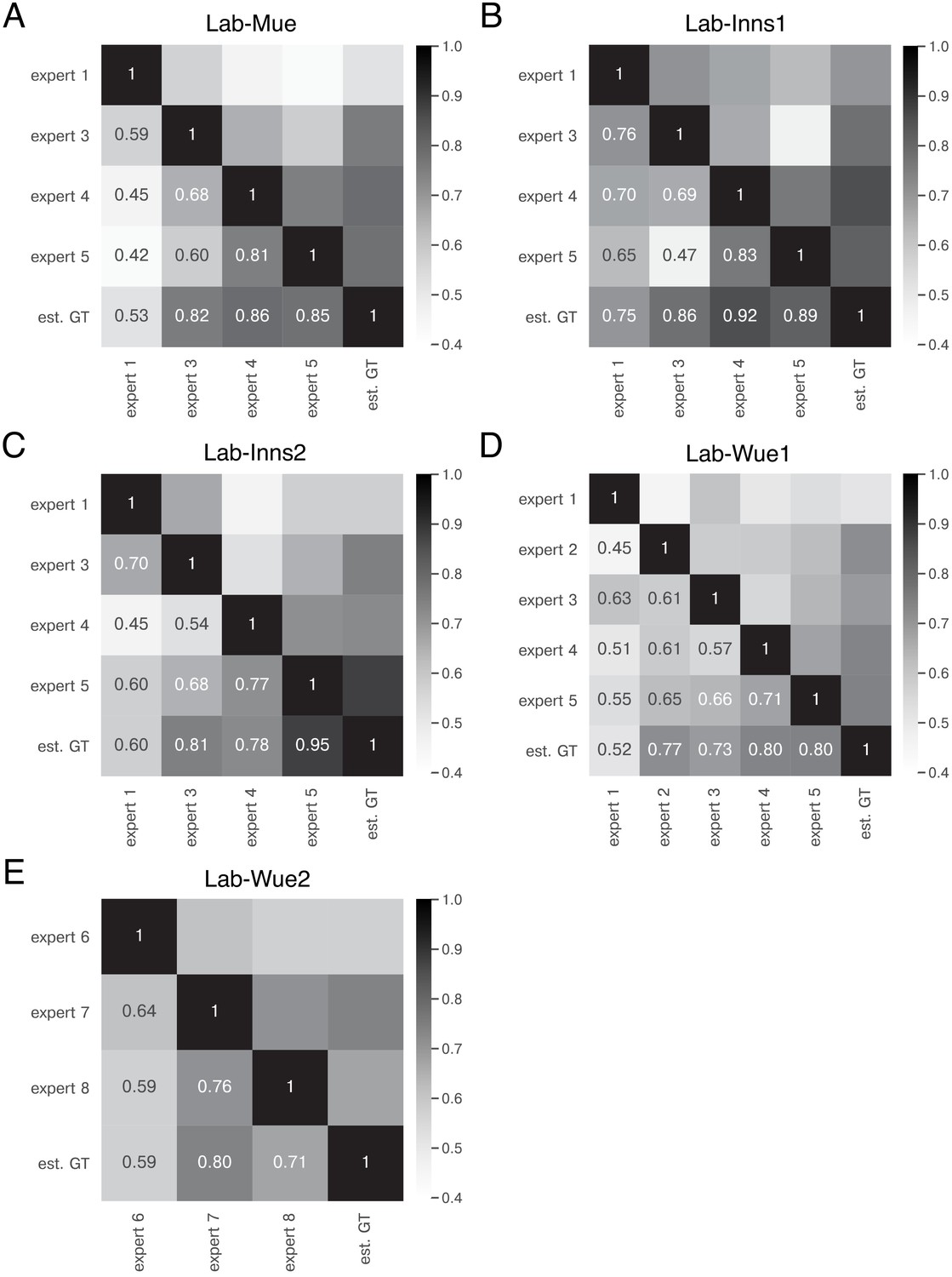
Expert similarity across all datasets: F1 scores.
The heatmaps show the mean of at a matching IoU-threshold of for the image feature annotations of the indicated experts. The estimated ground truth (est. GT) was always calculated on all available expert annotations. The expert number refers to a unique human annotator (e.g. expert 1 is the same person across the datasets in A-D). The similarity scores were calculated on n = 5 images for A,B,C, and E and n = 9 images (test set) for D. The similarity between the same experts varies across the datasets (A–D), indicating that the heuristic bias of the annotators depends on the underlying data. However, expert 1 consistently yields the lowest similarity scores A, C, and D. The overall performance between one group of experts remains within a similar range for different datasets (A–D) and is comparable for a second group of experts on a different image dataset (E).
Figure 5—figure supplement 4
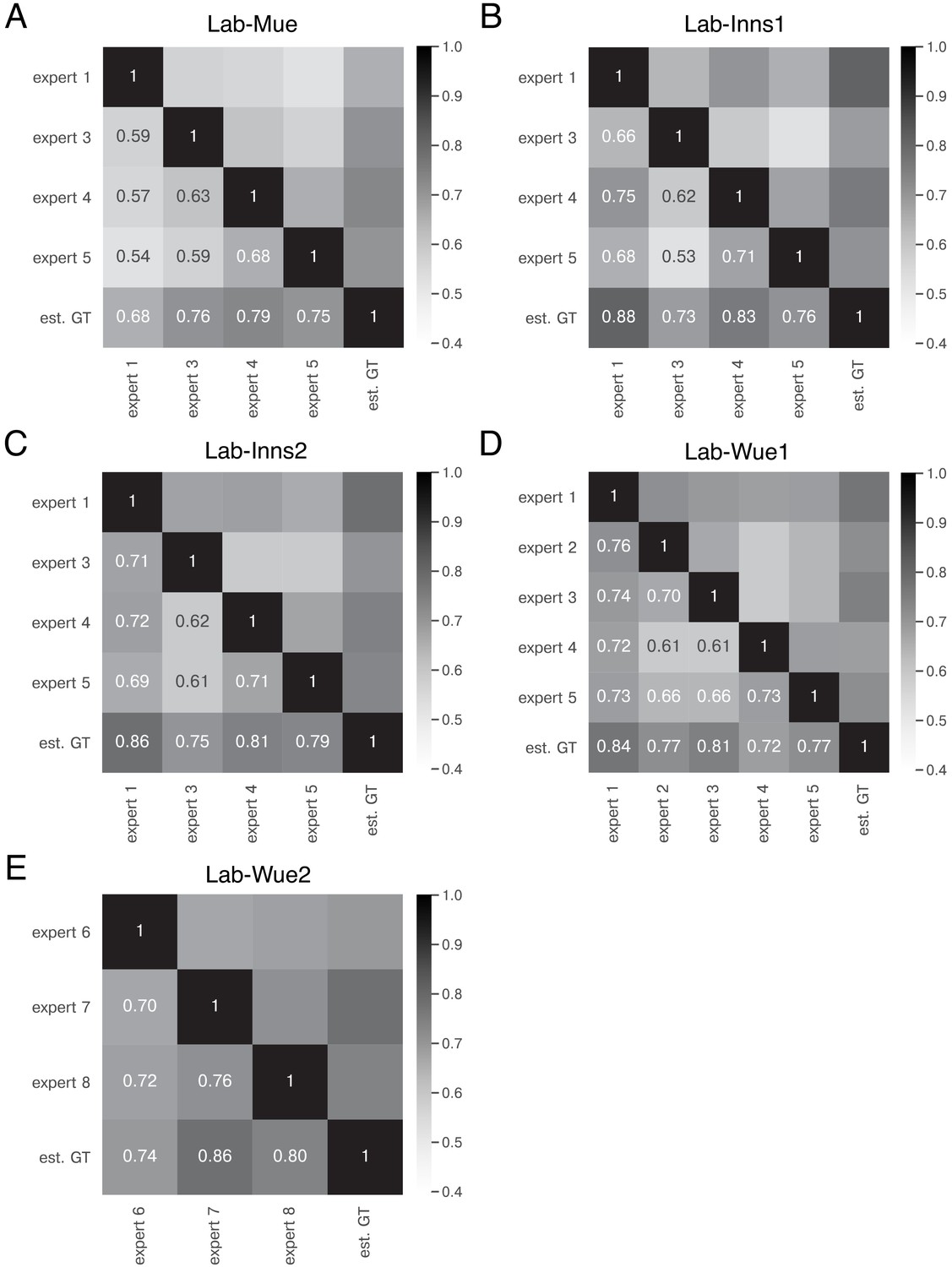
Expert similarity across all datasets: mean IoU.
The heatmaps show the mean of for the image feature annotations of the indicated experts. The estimated ground truth (est. GT) was always calculated on all available expert annotations. The expert number refers to a unique human annotator (e.g. expert 1 is the same person across the datasets in A-D). The similarity scores were calculated on n = 5 images for A, B, C, and E and n = 9 images (test set) for D. The similarity between the same experts varies across the datasets (A–D), indicating that the heuristic bias of the annotators depends on the underlying data. However, the overall performance between the experts remains within a similar range.
Figure 5—figure supplement 5
Reliability of the consensus approaches across different datasets.
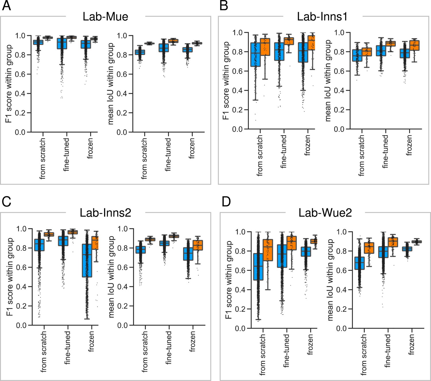
To asses the reliability and reproducibility of the consensus models and consensus ensembles strategies, we illustrate the within group at a matching IoU-threshold of and the within group across different datasets. Color coding refers to the different DL strategies: blue to consensus models; orange to consensus ensembles. All images used for training were excluded from the analysis. The differences between the datasets highlight the difficulties in establishing a unified approach for automated fluorescent label annotation. (A) The Lab-Mue analysis comprises n = 24 images and the following models: Nconsensus models = 12 and Nconsensus ensembles = 3 for all initialization variants. (B) The Lab-Inns1 analysis comprises n = 20 images and the following models: Nfrom scratch consensus models = 6, Nfine-tuned consensus models = 8, Nfrozen consensus models = 12, and Nconsensus ensembles = 3 for all initialization variants. (C) The Lab-Inns2 analysis comprises n = 25 images and the following models: Nfrom scratch consensus models = 15, Nfine-tuned consensus models = 15, Nfrozen consensus models = 12, and Nconsensus ensembles = 3 for all initialization variants. (D) The Lab-Wue2 analysis comprises n = 25 images and the following models: Nfrom scratch consensus models = 15, Nfine-tuned consensus models = 15, Nfrozen consensus models = 12, and Nconsensus ensembles = 3 for each initialization variant.
Tables
Table 1
Bioimage analyses results of external datasets.
Data are based either on manual analysis or on annotations by a consensus ensemble. The results are given for the individual consensus ensemble initialization variants (from scratch, fine-tuned). p-Values of Lab-Inns2 are corrected for multiple comparisons using Bonferroni correction. : mean group 1, : mean group 2, U: U-statistic, eRet: early retrieval, lRet: late retrieval, Ctrl: control, Ext: extinction, Sal: saline, Res: L-DOPA/MS-275 responder, nRes: L-DOPA/MS-275 non-responder, wt: wildtype, kd: gad1b knock-down.
| Lab | Groups | Initialization variant | U | Significance level (p) | |||
|---|---|---|---|---|---|---|---|
| Mue | eRet ∼ lRet | Manual | 1.00 | 1.65 | 19.0 | ** (0.002) | 0.39 |
| From scratch | 1.00 | 1.70 | 25.0 | ** (0.007) | 0.31 | ||
| Fine-tuned | 1.00 | 1.68 | 24.0 | ** (0.006) | 0.32 | ||
| Inns1 | Ctrl ∼ Ext | Manual | 1.00 | 3.92 | 10.0 | ** (0.005) | 0.43 |
| From scratch | 1.00 | 2.26 | 13.0 | * (0.010) | 0.35 | ||
| Fine-tuned | 1.00 | 1.85 | 14.0 | * (0.013) | 0.33 | ||
| Inns2 | Sal ∼ Resp | Manual | 1.00 | 1.83 | 5.0 | ** (0.002) | 0.59 |
| From scratch | 1.00 | 1.96 | 0.0 | *** (<0.001) | 0.71 | ||
| Fine-tuned | 1.00 | 2.07 | 0.0 | *** (<0.001) | 0.71 | ||
| Sal ∼ nResp | Manual | 1.00 | 1.05 | 27.0 | n.s. (1.000) | 0.00 | |
| From scratch | 1.00 | 1.63 | 8.0 | n.s. (0.130) | 0.29 | ||
| Fine-tuned | 1.00 | 1.42 | 12.0 | n.s. (0.377) | 0.16 | ||
| Res ∼ nRes | Manual | 1.83 | 1.05 | 42.0 | n.s. (0.130) | 0.29 | |
| From scratch | 1.96 | 1.63 | 41.0 | n.s. (0.173) | 0.26 | ||
| Fine-tuned | 2.07 | 1.42 | 42.0 | n.s. (0.130) | 0.29 | ||
| Wue2 | wt ∼ kd | Manual | 1.00 | 0.28 | 227.5 | * (0.010) | 0.19 |
| From scratch | 1.00 | 0.45 | 220.0 | * (0.021) | 0.16 | ||
| Fine-tuned | 1.00 | 0.37 | 216.0 | * (0.029) | 0.14 |
Key resources table
| Reagent type (species) or resource | Designation | Source or reference | Identifiers | Additional information |
|---|---|---|---|---|
| Genetic reagent (Mus musculus, male) | C57BL/6J | Charles River | Cat# CRL:027; RRID:IMSR_CRL:27 | Lab-Mue; Lab-Inns1 |
| Genetic reagent (Mus musculus, male) | C57BL/6J | Jackson Laboratory | Cat# JAX:000664; RRID:IMSR_JAX:000664 | Lab-Wue1 |
| Genetic reagent (Mus musculus, male) | 129S1/SvlmJ (S1) | Charles River | RRID:MGI:5658424 | Lab-Inns2 |
| Genetic reagent (Danio rerio) | AB/AB | European Zebrafish Resource Center | Lab-Wue2 | |
| Antibody | Anti-cFOS (rabbit polyclonal) | Santa Cruz | Cat# sc-52; RRID:AB_2106783 | Lab-Mue (1:500); Lab-Inns2 (1:1,000) |
| Antibody | Anti-cFOS (rabbit polyclonal) | Millipore | Cat# PC38; RRID:AB_2106755 | Lab-Inns1 (1:20,000) |
| Antibody | anti-cFOS (rabbit polyclonal) | Synaptic Systems | Cat# 226003; RRID:AB_2231974 | Lab-Wue1 (1:10,000) |
| Antibody | Anti-GABA (rabbit polyclonal) | Sigma-Aldrich | Cat#A2025; RRID:AB_477652 | Lab-Wue2 (1:400) |
| Antibody | Anti-NeuN (guinea-pig polyclonal) | Synaptic Systems | Cat# 266004; RRID:AB_2619988 | Lab-Wue1 (1:400) |
| Antibody | Anti-Parvalbumin (mouse monoclonal) | Sigma-Aldrich | Cat# P3088; RRID:AB_477329 | Lab-Inns1 (1:2,500) |
| Antibody | Anti-Parvalbumin (mouse monoclonal) | Swant | Cat# PV235; RRID:AB_10000343 | Lab-Wue1 (1:5,000) |
| Software, algorithm | ImageJ | Fiji www.fiji.sc/ | RRID:SCR_002285 | Lab-Mue; Lab-Inns2; Lab-Wue1; Lab-Wue2 |
| Software, algorithm | Improvision Openlab software | Perkin Elmer www.perkinelmer.com/ pages/020/cellularimaging/ products/openlab.xhtml | RRID:SCR_012158 | Lab-Inns1, Version 5.5.0 |
| Software, algorithm | GraphPad Prism software | GraphPad Prism www.graphpad.com/ scientific-software/prism/ | RRID:SCR_015807 | Lab-Inns1, Version 7.0 |
| Software, algorithm | CellSens Dimension Desktop software | Olympus www.olympus-lifescience.com/ en/software/cellsens/ | RRID:SCR_016238 | Lab-Inns2, Version 1.9 |
| Software, algorithm | Fluoview FV10-ASW | Olympus www.photonics.com/ Product.aspx?PRID=47380 | RRID:SCR_014215 | Lab-Wue1 |
| Software, algorithm | Tensorflow | www.tensorflow.org, Abadi et al., 2016 | RRID:SCR_016345 | |
| Software, algorithm | Keras | www.keras.io, Chollet, 2015 | ||
| Software, algorithm | Imagej | www.imagej.net/, Rueden et al., 2017 | RRID:SCR_003070 | |
| Software, algorithm | SciPy | www.scipy.org, Jones et al., 2001 | RRID:SCR_008058 | |
| Software, algorithm | scikit-learn | www.scikit-learn.org/, Pedregosa et al., 2011 | ||
| Software, algorithm | scikit-image | www.scikit-image.org/, van der Walt et al., 2014 | ||
| Software, algorithm | Pingouin | https://pingouin-stats.org/, Vallat, 2018 | ||
| Software, algorithm | simpleITK | www.simpleitk.org/, Lowekamp et al., 2013 |
Additional files
Download links
A two-part list of links to download the article, or parts of the article, in various formats.
Downloads (link to download the article as PDF)
Open citations (links to open the citations from this article in various online reference manager services)
Cite this article (links to download the citations from this article in formats compatible with various reference manager tools)
On the objectivity, reliability, and validity of deep learning enabled bioimage analyses
eLife 9:e59780.
https://doi.org/10.7554/eLife.59780


