Investigating the trade-off between folding and function in a multidomain Y-family DNA polymerase
- Department of Chemistry, State University of New York at Stony Brook, United States
- Department of Biomedical Sciences, College of Medicine, Florida State University, United States
Figures
Figure 1 with 1 supplement
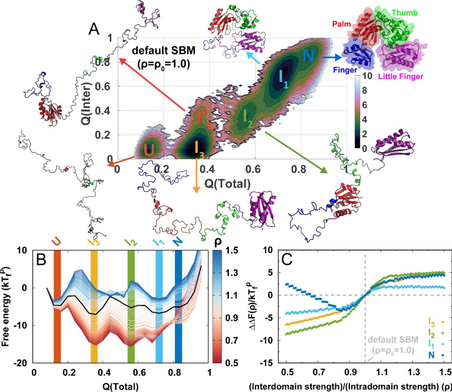
DPO4 folding thermodynamics.
(A) The 2D folding free energy landscape of DPO4 projected onto the fractions of total () and interdomain () native contacts for the default SBM parameter at the folding temperature . There are six folding states identified on the free energy landscape, which are denoted by , , , , , and , with corresponding typical DPO4 structures shown. The all-atom representations of DPO4 were reconstructed based on the structures from the simulations (Rotkiewicz and Skolnick, 2008). Domains of DPO4 are labeled with different colors: the finger domain (F, blue, residues 11–77), the palm domain (P, red, residues 1–10 and 78–166), the thumb domain (T, green, residues 167–229), the little finger domain (LF, purple, residues 245–341), and the flexible linker (gray, residues 230–244), which connects the T and LF domains. (B) The 1D folding free energy landscape of DPO4 projected onto for different values of the ratio of interdomain to intradomain native contact strength, denoted by ρ and ranging from 0.5 to 1.5 (indicated by different colors). It is worth noting that the and states cannot be distinguished by . The black line corresponds to the free energy landscape for the default SBM parameter . We set the zeros of the free energies at the lowest detected from the simulations. (C) Change in stability of each folding state for ρ relative to that for at the corresponding folding temperature according to the expression , where represents the folding state (, , , or ) and is the stability of the folding state at ρ. is calculated as the free energy difference between the folding state and the unfolded state , where is the free energy obtained from (B).
Figure 1—figure supplement 1
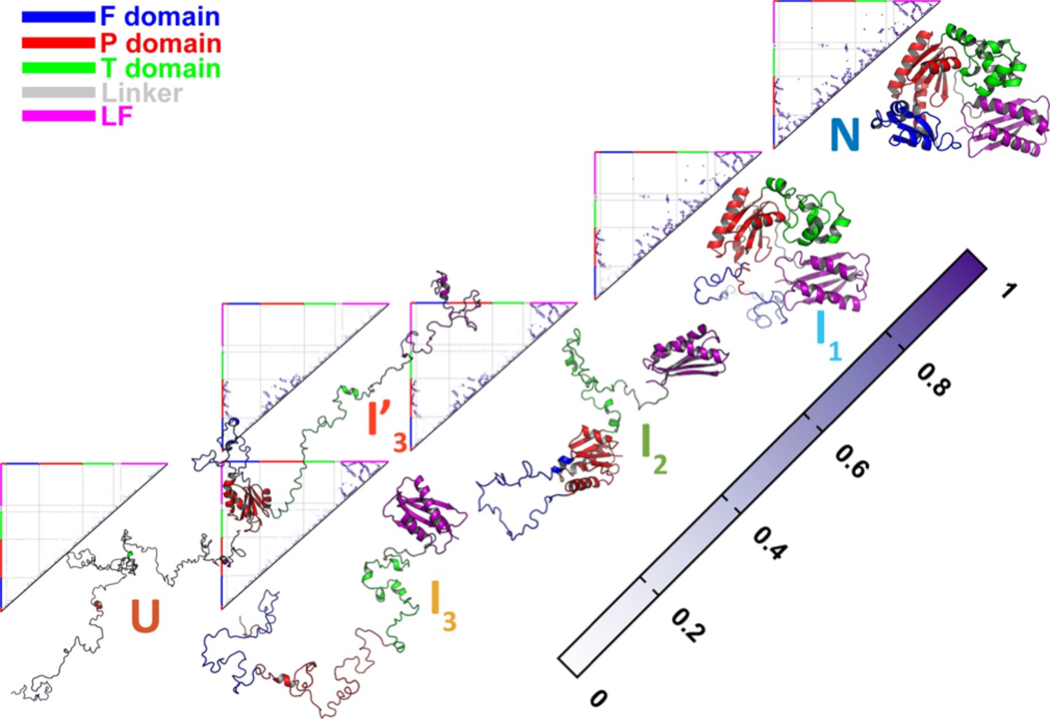
Native contact maps of DPO4 for the folding states , , , , , and .
Native contact maps of DPO4 for the folding states , , , , , and at the folding temperature .
Figure 2 with 7 supplements

DPO4 folding free energy landscapes, backtracking, and folding cooperativity for different values of ρ.
(a, B) 2D folding free energy landscapes of DPO4 for (A) and (B) . (C) Averaged versus for different values of ρ at the corresponding folding temperature calculated from the 2D free energy landscapes. The black line corresponds to the result with the default parameter . The two shaded regions show the increase followed by the decrease in with increasing for ρ close to its default value , indicating possible backtracking during DPO4 folding. (D) Averaged versus at a temperature and for the default parameter , as calculated from the kinetic simulations. The colored lines are the observations for the individual folding events in all the simulations (a total number of 100), and the black line indicates the average. The domain structure in DPO4 in the backtracking regions is described by the fractions of native contacts , , , and , the last two of which are shown in (E) and (F), respectively. There are two separate regions in backtracking region II, implying two distinct DPO4 structures. (G) Thermodynamic coupling index () for the default parameter . (H) Dependence of the mean thermodynamic coupling index () on ρ. The black and gray lines show the of the intact DPO4 and the four domains in DPO4, respectively. The dashed line indicates the calculated from the independent folding simulations of the four domains of DPO4, reminiscent of the extreme case with .
Figure 2—figure supplement 1
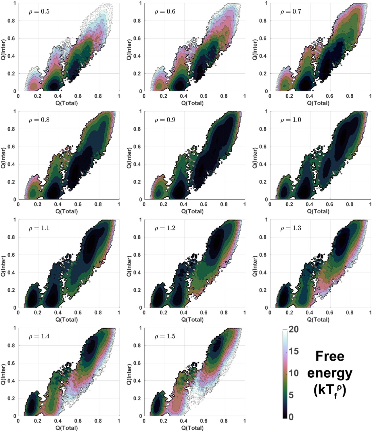
2D free energy landscapes for DPO4 folding with different values of ρ.
2D folding free energy landscapes of DPO4 for different values of ρ at the corresponding folding temperatures .
Figure 2—figure supplement 2
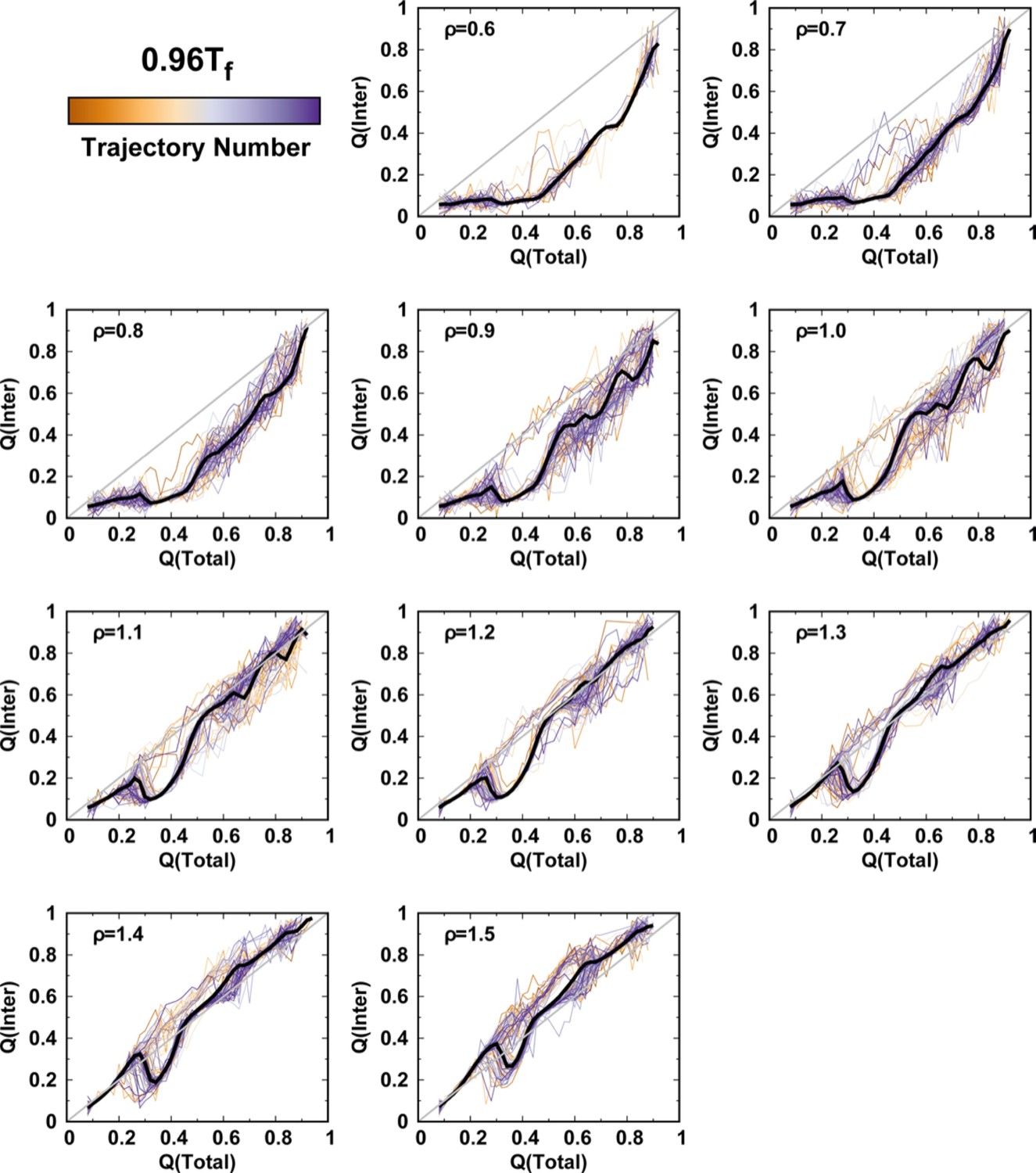
Averaged and at a temperature for different values of ρ.
One hundred independent simulations starting from different unfolded states of DPO4 for each value of ρ.
Figure 2—figure supplement 3
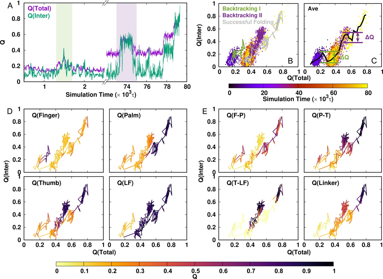
Representative DPO4 folding trajectory to illustrate backtracking.
(A) DPO4 folding trajectory projected onto and . The two shaded regions represent two backtracking processes. (B) DPO4 folding trajectory, including two backtracking and one successful folding processes. (C) Averaged versus . The magnitude of the increase relative to the subsequent decrease in as increases, which is denoted by , is used to characterize the backtracking process. (In practice, we define backtracking by .) The backtracking and folding processes are shown in terms of the fraction of each intradomain folding (D) and interdomain formation (E).
Figure 2—figure supplement 4
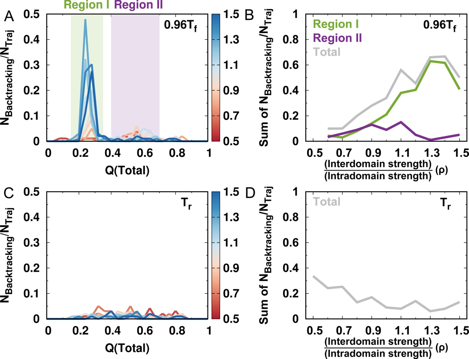
Number of backtracking observed for different values of ρ.
(A) Number of backtracking observed versus for different values of ρ. is the number of backtracking characterized by the averaged and (Figure 2—figure supplement 3) and is the number of folding events in the simulations at a temperature . (B) Number of backtracking occurring in various regions for different values of ρ. (C) and (D) are the same as (A) and (B), but at room temperature .
Figure 2—figure supplement 5

Native contact maps and structures of DPO4 at backtracking.
All-atom representations of DPO4 reconstructed based on the structures from the simulations (Rotkiewicz and Skolnick, 2008).
Figure 2—figure supplement 6
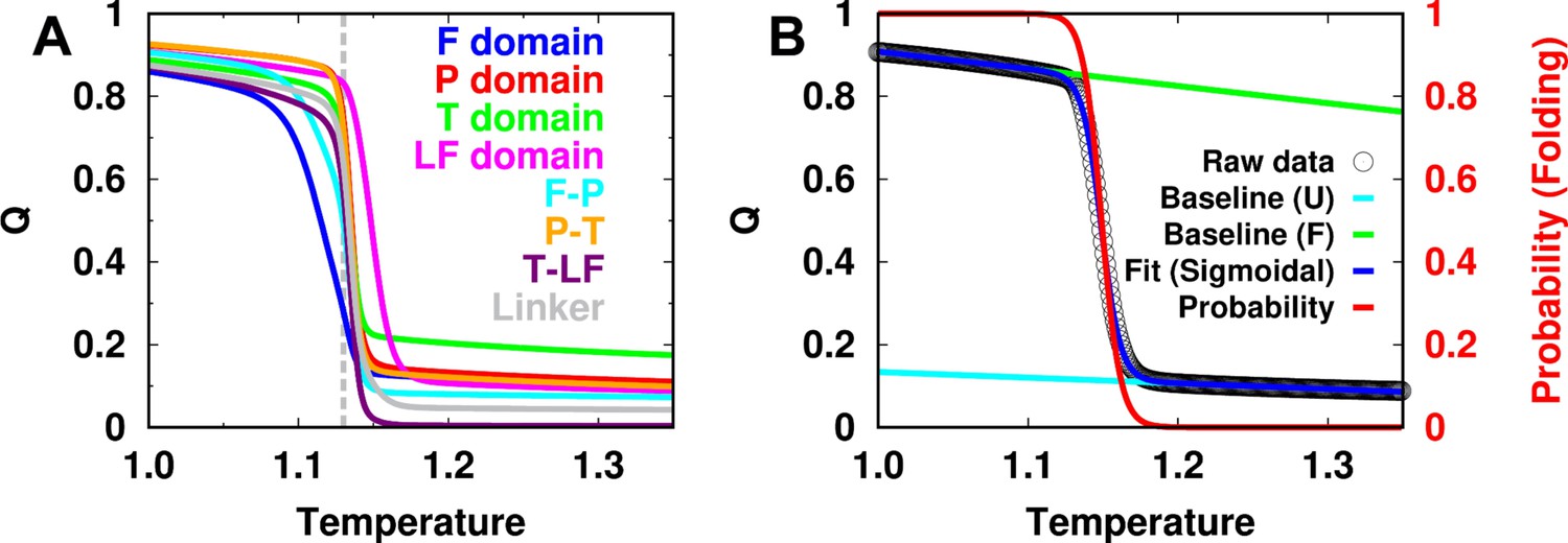
Melting curve of each domain/interface and two-state sigmoidal fitting.
(A) Melting curves of Q for each intradomain, interdomain, and linker of DPO4 for . The dashed line indicates the folding temperature. (B) One example of a melting curve of the P domain of DPO4 and its fitting to the two-state sigmoidal transition to obtain the folding probability curve , where I is the index of the intra- or interdomain and T is the temperature. The data for the P domain shown here are chosen for the purposes of illustration. Similar results can be observed for the other intra- and interdomains for different values of ρ. The fitting procedure follows the standard protocol instructed by Sborgi et al., 2012.
Figure 2—figure supplement 7
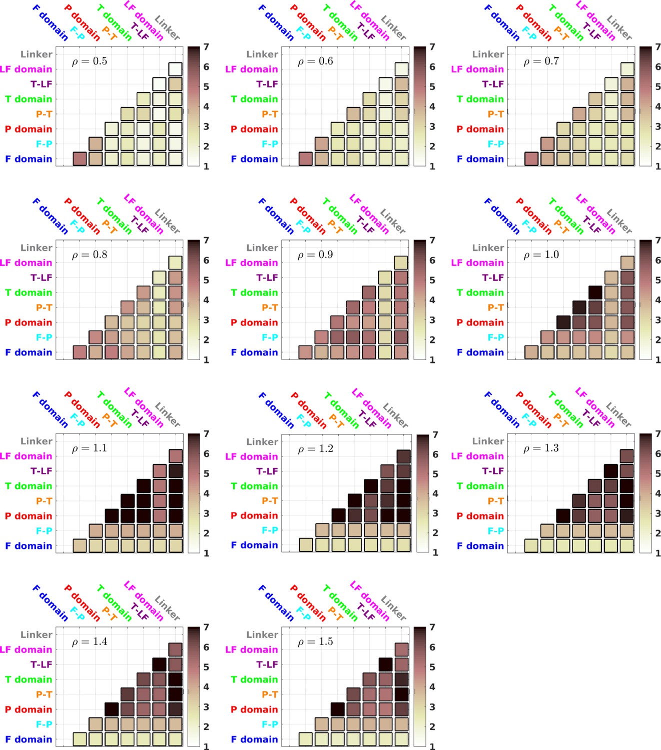
TCI for different values of ρ.
between different domains/interfaces for different values of ρ.
Figure 3 with 3 supplements
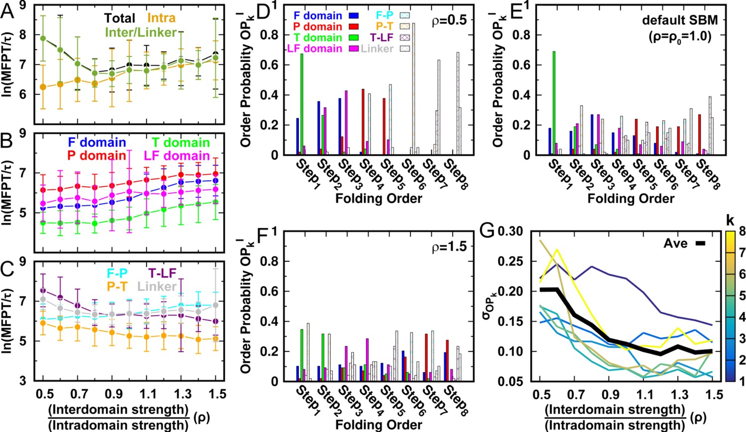
DPO4 folding kinetics at room temperature .
(A–C) Kinetic rates quantified by the mean first passage time (MFPT) for (A) intradomain, interdomain, and total folding, (B) individual intradomain folding, and (C) interdomain formation. MFPT is in units of τ, which is the reduced time unit used in our simulations. Error bars represent the standard deviations at the corresponding MFPT. A folding is defined as when the corresponding Q is higher than 0.75. (D–F) Folding order probability of individual intra- and interdomain occurs during a successful DPO4 folding event with (D) , (E) the default parameter , and (F) . k is the order index of the folding step and is the index of the domain/interface of DPO4. There are eight domains/interfaces in DPO4, and thus eight folding steps are defined. (G) Standard deviation of from its mean at folding step for different values of ρ. The black line shows the average versus ρ.
Figure 3—figure supplement 1
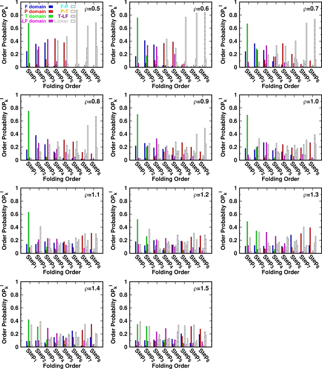
for different values of ρ.
Folding order probability of intra- and interdomains for different values of ρ.
Figure 3—figure supplement 2
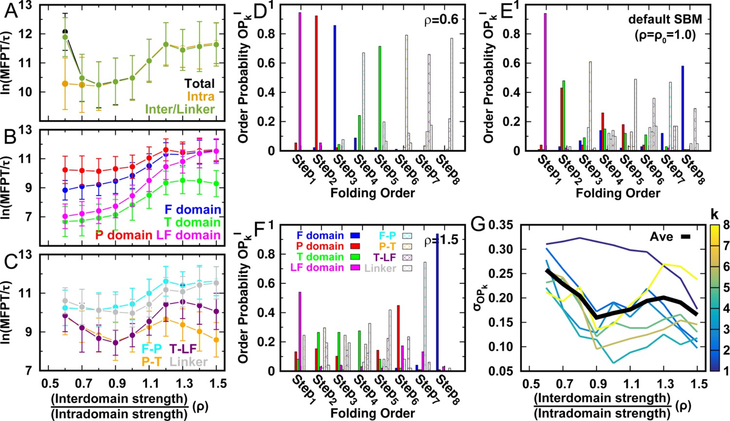
DPO4 folding kinetics at a temperature .
Kinetic rates and folding order of individual domains/interfaces during a successful DPO4 folding event for different values of ρ at a temperature . The data at are absent because an SBM with such a parameter value could not accumulate a statistically sufficient number of folding events for analysis.
Figure 3—figure supplement 3
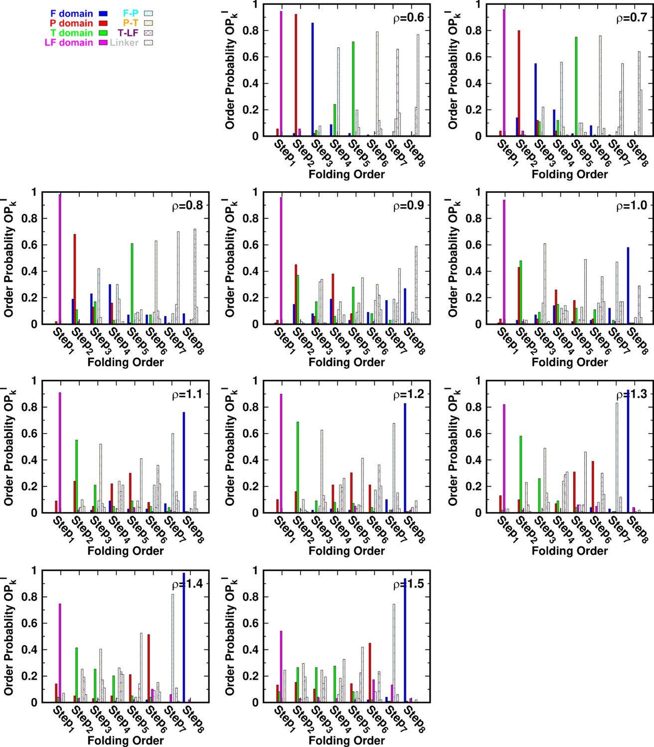
for different values of ρ at a temperature .
Folding order probability of intra- and interdomains for different values of ρ at a temperature .
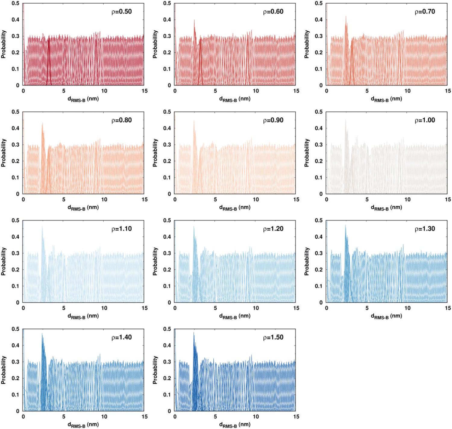
Figure 4 with 5 supplements
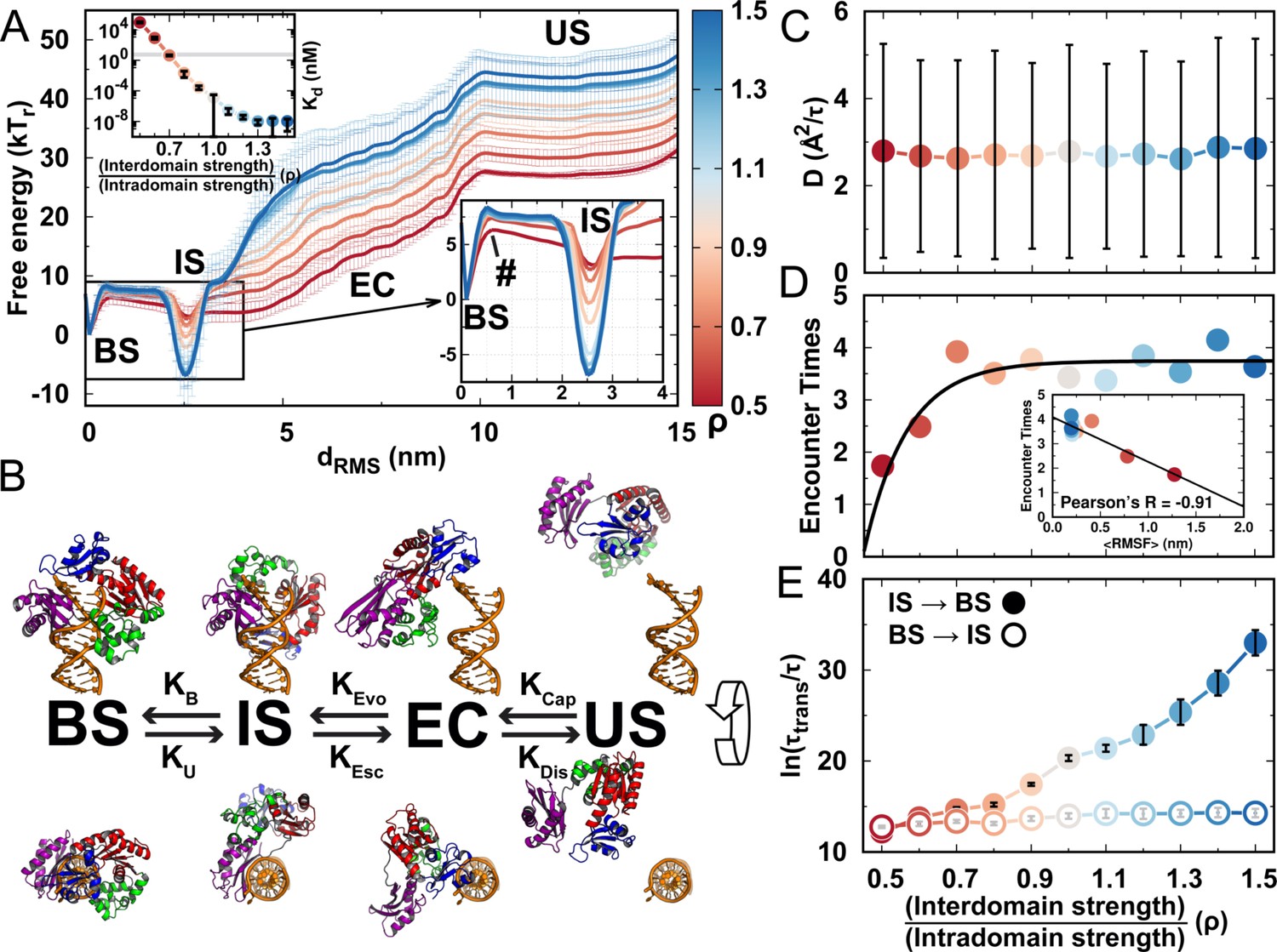
DPO4–DNA binding thermodynamics and kinetics.
(A) 1D free energy landscape of DPO4–DNA binding versus the distance root-mean-square deviation of DPO4–DNA binding native contacts for different values of ρ. has units of length and deviates from 0 nm as unbinding proceeds. The binding process can be divided into four states: US, EC, IS, and BS. The insert at the top left shows the binding affinity for different values of ρ, with the gray line corresponding to the experimental measurements (3–10 nM). The insert at the bottom right is a magnified view of the binding free energy landscape focusing on the transition between the BS and the IS. The error analysis was done by performing four independent umbrella sampling simulations with different initial conditions. Error bars are omitted from this insert for clarity. (B) The four-state DPO4–DNA binding process. Typical corresponding DPO4–DNA structures obtained from the simulations for different binding states are shown from two perpendicular viewpoints. There are three transitions in the four-state DPO4–DNA binding process. The ρ-dependent DPO4–DNA binding kinetics in terms of these three transitions are shown in (C–E). (C) Diffusion coefficient D of free DPO4 (in the absence of DNA) for different values of ρ. D reflects the essence of . Error bars represent the standard deviations from the corresponding mean values of D. τ is the reduced time unit. (D) Encounter times of the EC evolving to the IS with different values of ρ. The encounter time was calculated from the expression . The insert is a plot of encounter times versus the mean root-mean-square fluctuation () of DPO4 in the free state. The mean was obtained from the free DPO4 simulations by averaging all the residues in DPO4 (Figure 4—figure supplement 3). (E) Transition times between the BS and the IS for different values ρ. was calculated from 100 independent simulations, and the errors were estimated by a bootstrap analysis with 50 subsamples.
Figure 4—figure supplement 1
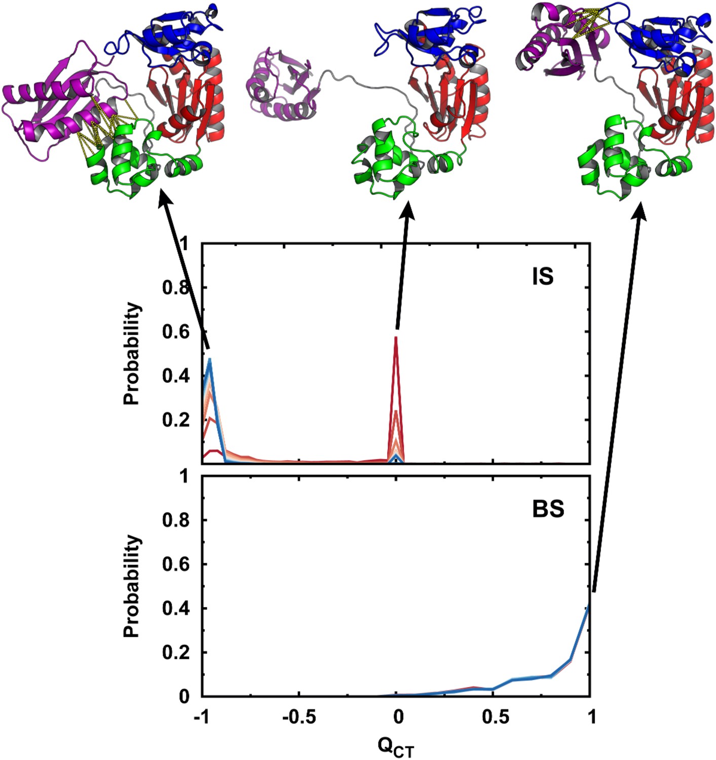
Conformational distributions of DPO4 in the IS and BS.
Conformational distributions of DPO4 in the IS and BS during the DNA-binding process. is defined as , where is the fraction of native contacts between the T and LF domains in the apo-DPO4 structure and is the fraction of native contacts between the F and LF domains in the binary DPO4–DNA structure. when DPO4 is in the apo form, and when DPO4 is in the binary form. DPO4 with has fully broken the LF interdomain interaction and thus possesses an extended LF domain with flexible linker. Typical structures of DPO4 are shown for illustration at , 0.0, and 1.0. The native contacts of the LF interdomain are shown when and 1.0 by the yellow dashed lines.
Figure 4—figure supplement 2

Free DPO4 diffusion for different values of ρ.
(A) Distributions of the diffusion coefficient of DPO4 for different values of ρ. is calculated as , where is the mean square displacement (MSD) for the center of mass of DPO4 with respect to the initial reference structure. In practice, was calculated directly by using the command “” implemented in Gromacs (4.5.7) (Hess et al., 2008). 1000 trajectories (each long, giving an accumulated length of ) were used for each value of ρ to calculate . (B) The most probable obtained from (A) for different values of ρ. The values of the most probable at different values of ρ are very similar.
Figure 4—figure supplement 3
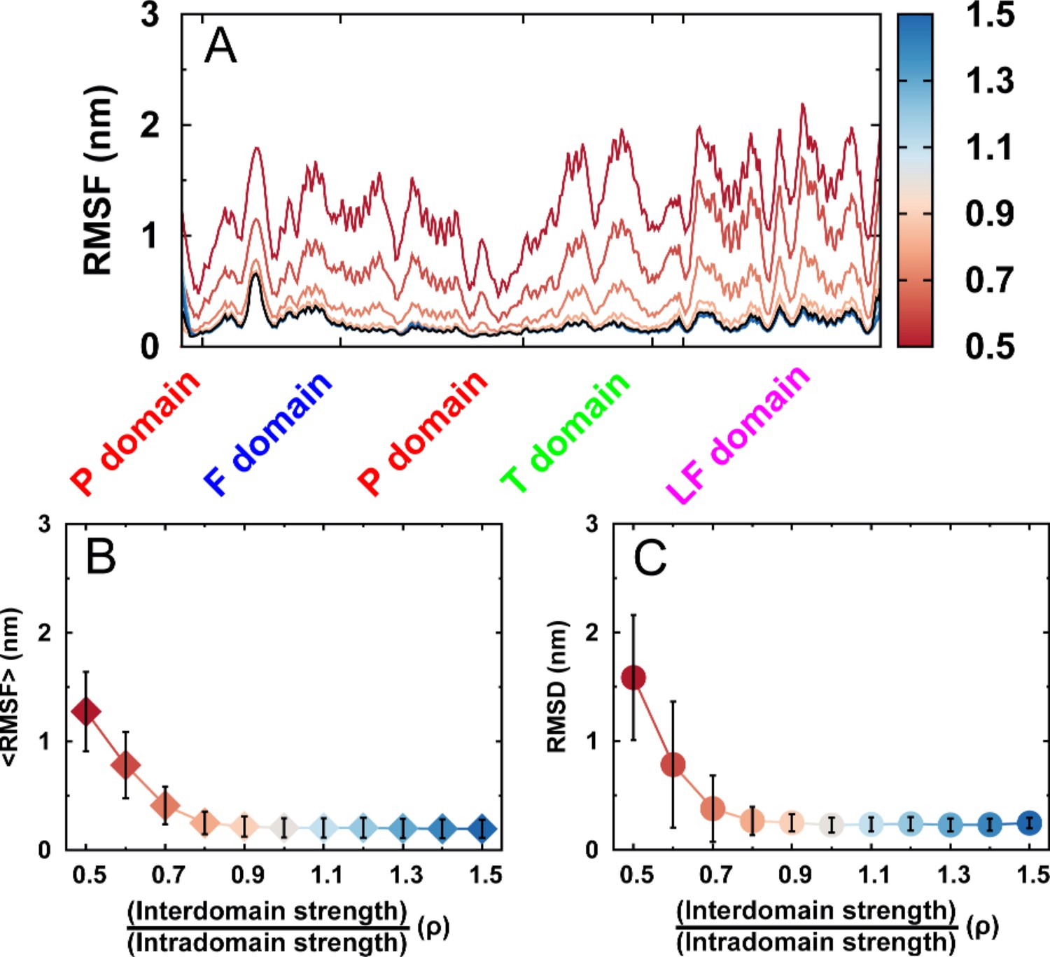
Structural fluctuations of free DPO4 for different values of ρ.
Structural fluctuations of free DPO4 for different values of ρ in terms of (A) RMSF, (B) mean RMSF averaged over all residues, and (C) RMSD from the native PDB structure. Error bars represent the standard deviations from the corresponding mean values.
Figure 4—figure supplement 4
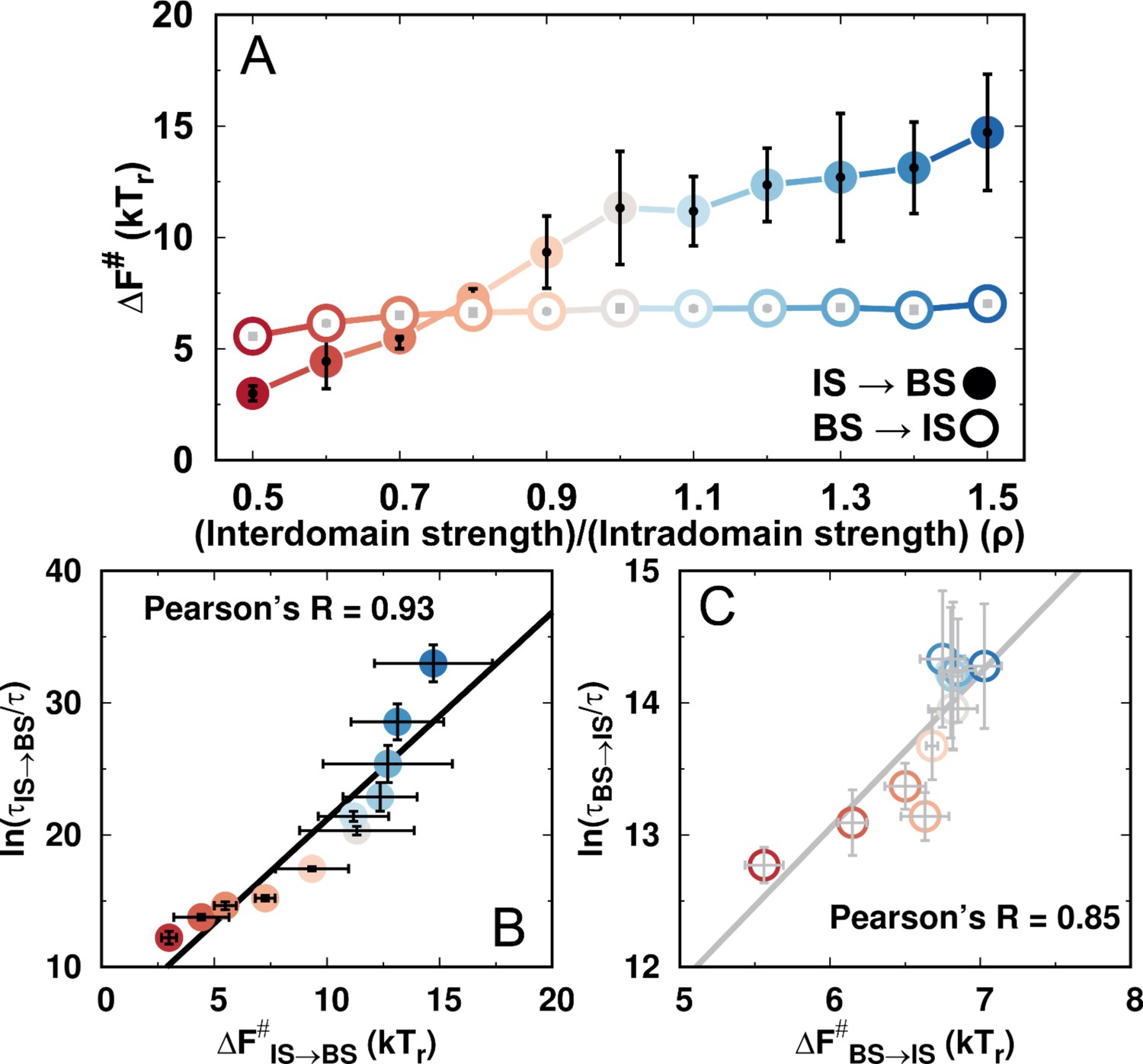
Thermodynamic barrier heights and kinetic times for the transitions between the IS and the BS during DPO4–DNA binding for different values of ρ.
(A) Free energy barriers of the transitions between the IS and the BS for different values of ρ. The error bars represent the standard deviations from the corresponding mean values. (B, C) Correlations between thermodynamic free energy barrier heights and kinetic times for transitions (B) from the IS to BS and (C) from the BS to the IS for different values of ρ.
Figure 4—figure supplement 5
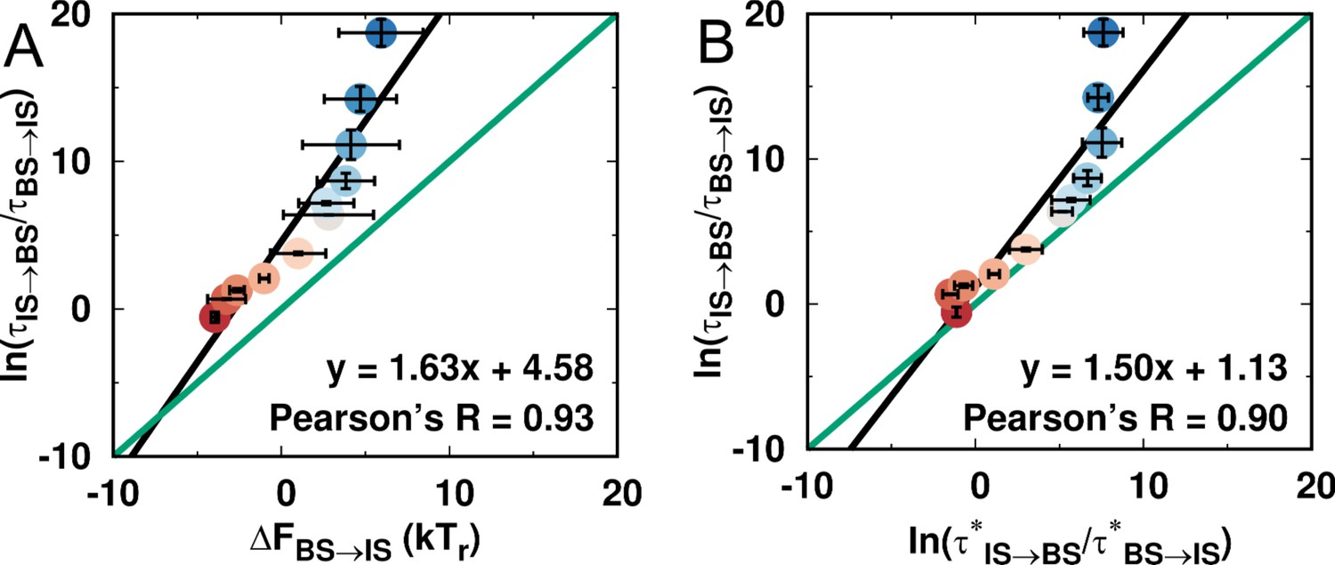
Comparison of thermodynamic and kinetic stabilities of the IS and BS during DPO4–DNA binding for different values of ρ.
A direct comparison between the thermodynamic and kinetic results can be made by comparing the thermodynamic and kinetic stabilities as suggested previously (Wang et al., 2017). The thermodynamic stability is defined as , where is the free energy obtained from the free energy landscape, while the kinetic stability is defined as , where is the transition time calculated from the kinetic simulations. (A) Correlation between thermodynamic and kinetic stability. (B) Correlation between the kinetic stabilities of the IS and BS. was calculated from the free energy landscape (see Appendix 1) and thus is the result from the thermodynamic simulation.
Figure 5
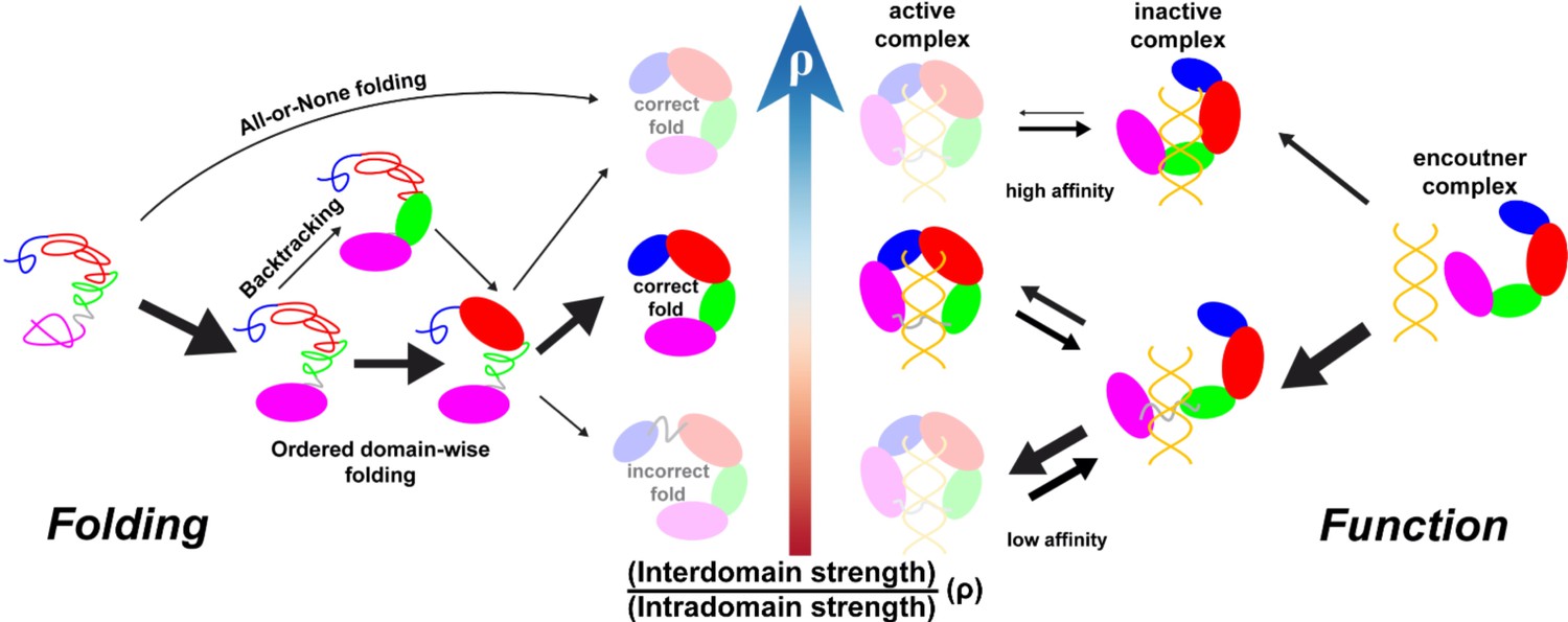
Illustration of intra- and interdomain interactions in the trade-off between DPO4 folding and function.
The four domains of DPO4 are indicated using the same color scheme as in Figure 1A. The sizes of the arrows indicate the magnitudes of the rates or fluxes for folding (binding). DPO4 and DPO4–DNA binding complexes shown in lighter shades are less stable or populated than the others.
Appendix 3—figure 1
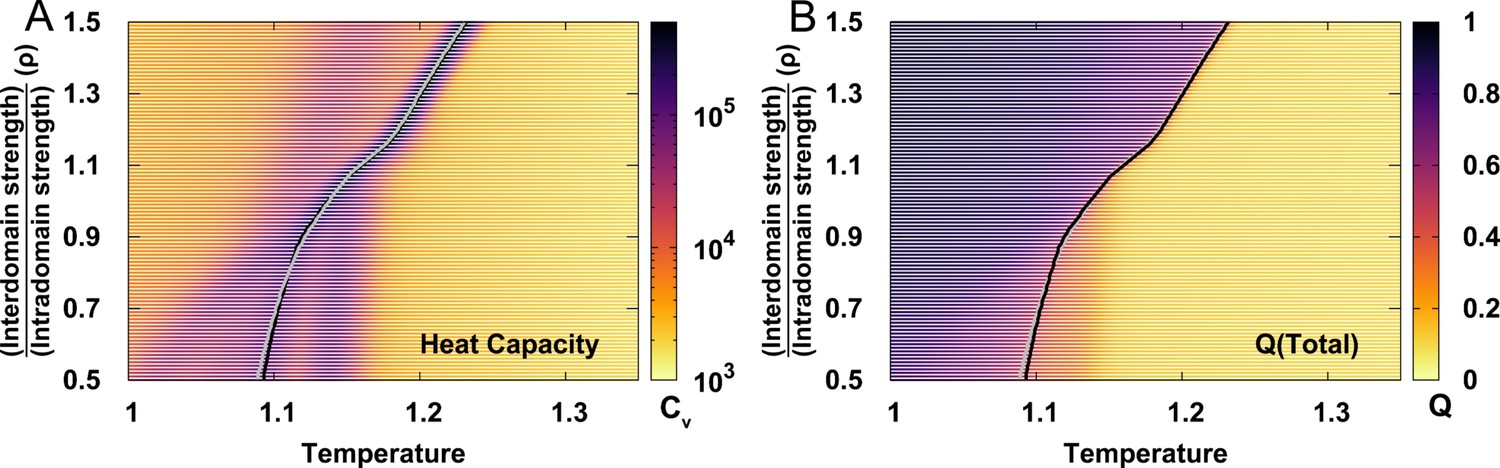
Extracting folding temperature from the heat capacity curves and melting curves of for different values of .
can be determined as the position of the prominent peak on heat capacity curve (black lines) or the midpoint of melting curves of (grey lines).
These two methods generate very similar , so from heat capacity was finally chosen.
Appendix 3—figure 2
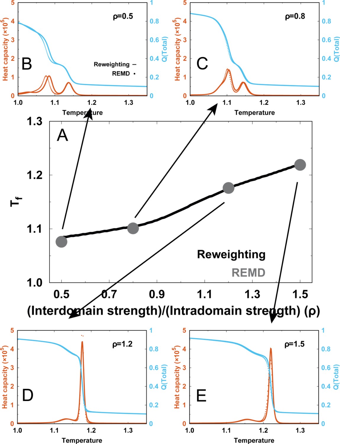
Comparisons of the thermodynamics between the reweighing method (solid lines) and direct REMD simulations (dots).
(A) Comparisons of folding temperatures. The REMD simulations with directly applying four different , which are (B) , (C) , (D) and (E) , were performed and analyzed. In (B-E), comparisons of heat capacity curves (blue) and melting curves of (red) with these four different are shown.
Appendix 3—figure 3
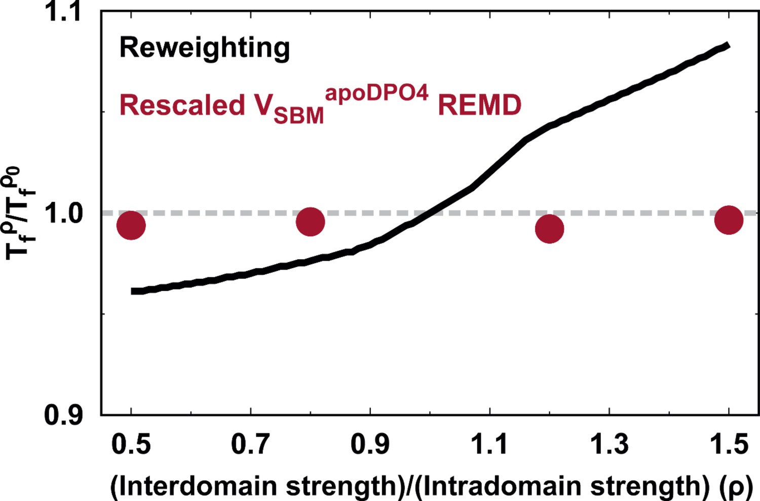
Assessment of shifting folding temperature with to that with the default parameter in order to perform kinetic simulations.
Comparisons are made between the reweighting method and the direct REMD simulations with rescaled .
Appendix 3—figure 4

Folding thermodynamics of intradomain in DPO4.
(A) Folding free energy landscapes of intradomain in DPO4 for different values of . Temperatures are the corresponding folding temperatures varied by different . Folded and unfolded states are marked at the Q with the free energy minima. (B) The stability of the folded states to unfolded states varied by different . The stability is defined as the free energy difference between the folded and unfolded states, obtained in (A).
Appendix 3—figure 5
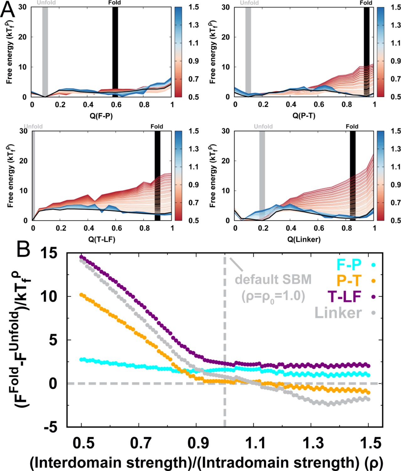
Folding thermodynamics of interdomain in DPO4.
(A) Folding free energy landscapes of interdomain in DPO4 for different values of . (B) The stability of the folded states to unfolded states varied by different .
Appendix 3—figure 6
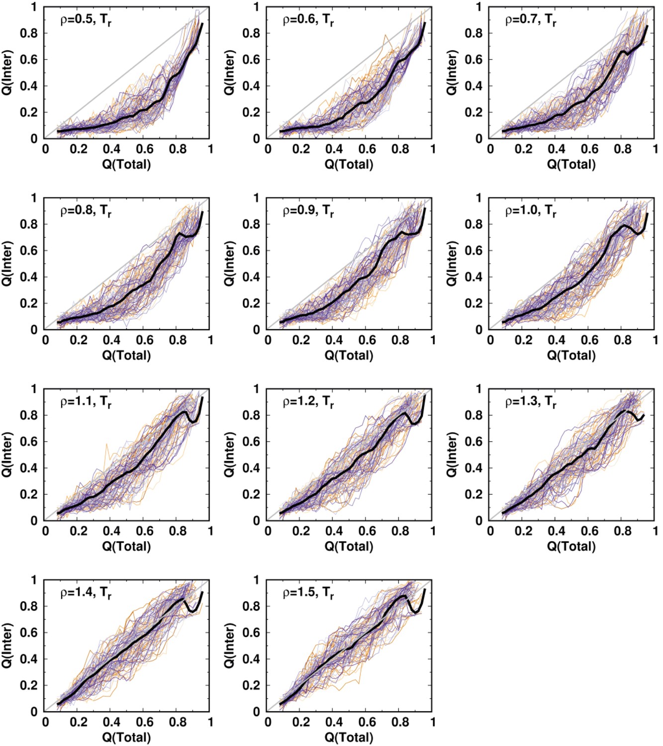
The averaged along with at temperature for different values of .
Appendix 3—figure 7
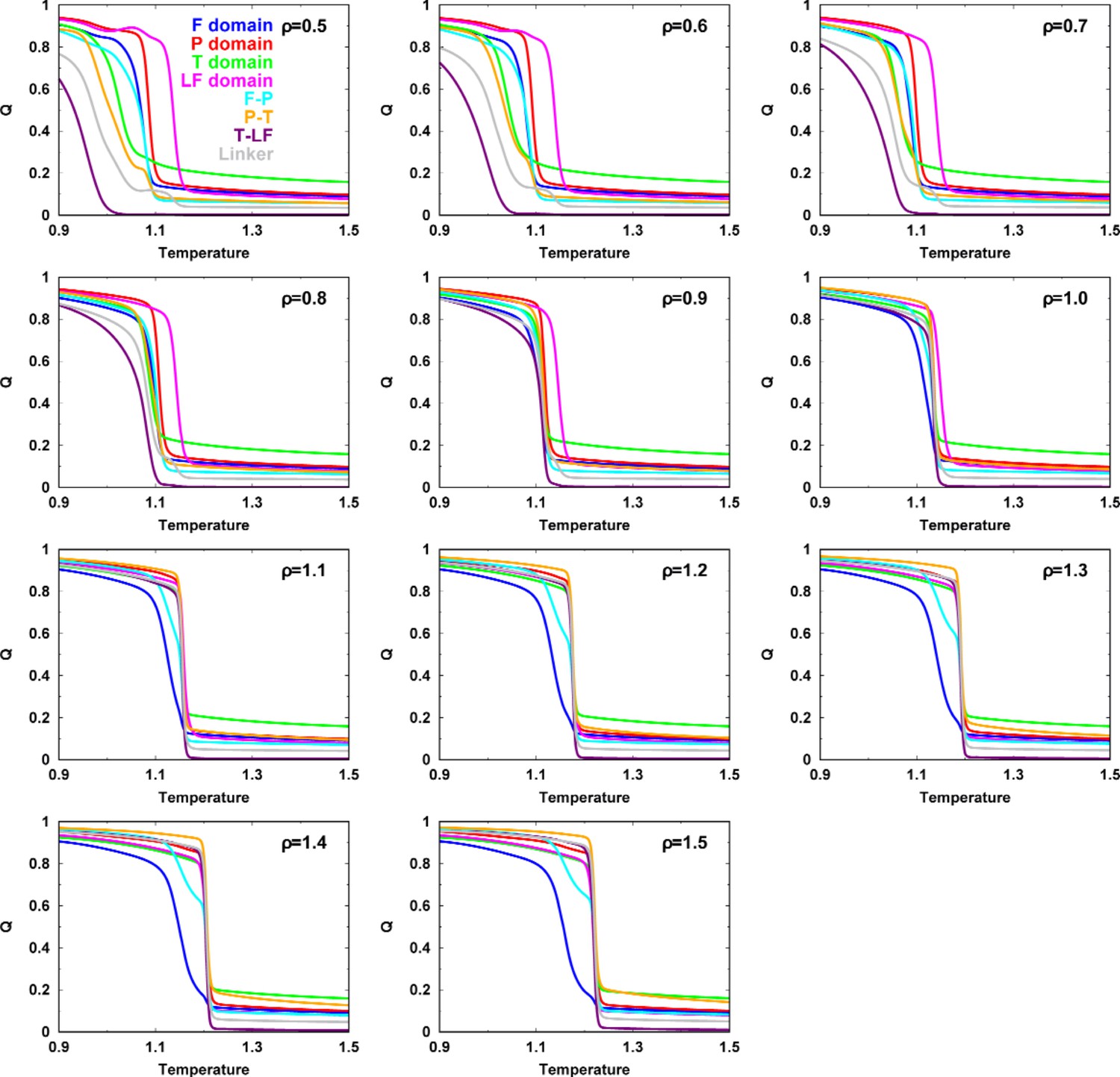
Melting curves of Q for each intra-, interdomain of DPO4 for different values of .
Appendix 3—figure 8
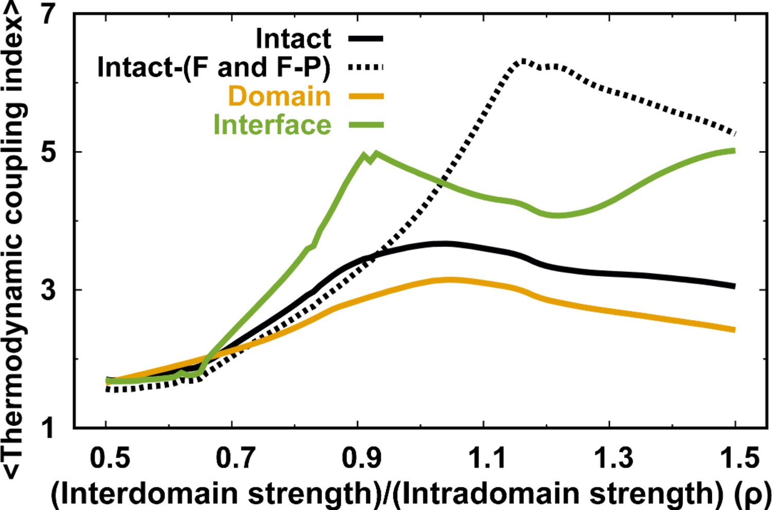
MTCI along with .
The dashed line represents the MTCI of removing the melting curves of the F and F-P from the intact DPO4.
Appendix 3—figure 9
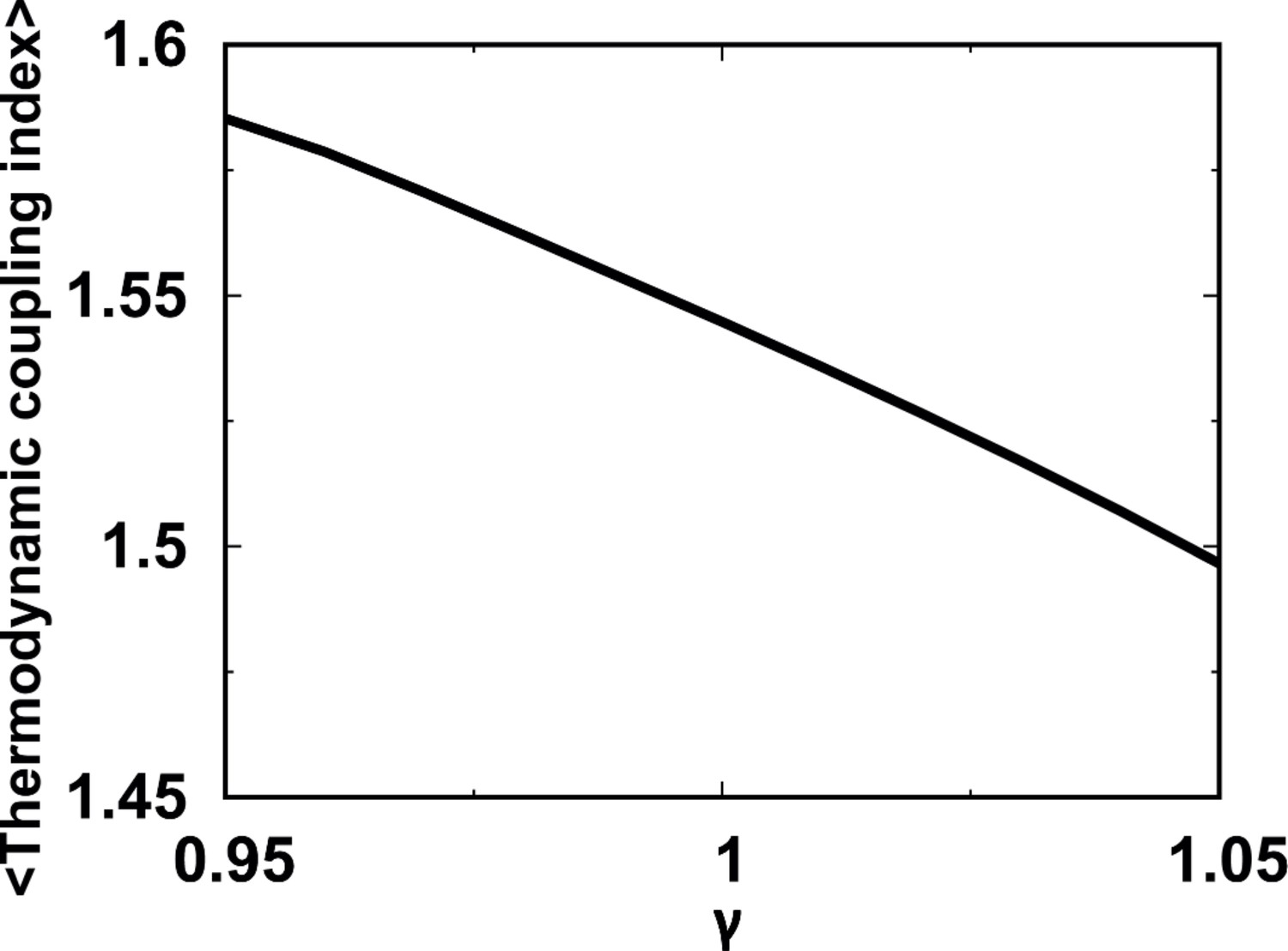
MTCI for independent folding of the four individual domains with different strengths of modulated by a pre-factor .
The reweighting method is used for calculations of MTCI at different via the REMD simulations performed at .
Appendix 3—figure 10

The coarse-grained structures for the P domain from PDB (left) and modeling (right).
Five glycines were added to connect the residue 10 to 77. The structure was used for the independent folding simulation of the P domain.
Appendix 3—figure 11
Biased DPO4–DNA binding simulations performed by the umbrella sampling.
The overall overlaps of the probability distribution on between neighboring replicas are apparent, indicating a sufficient sampling.
Appendix 3—figure 12
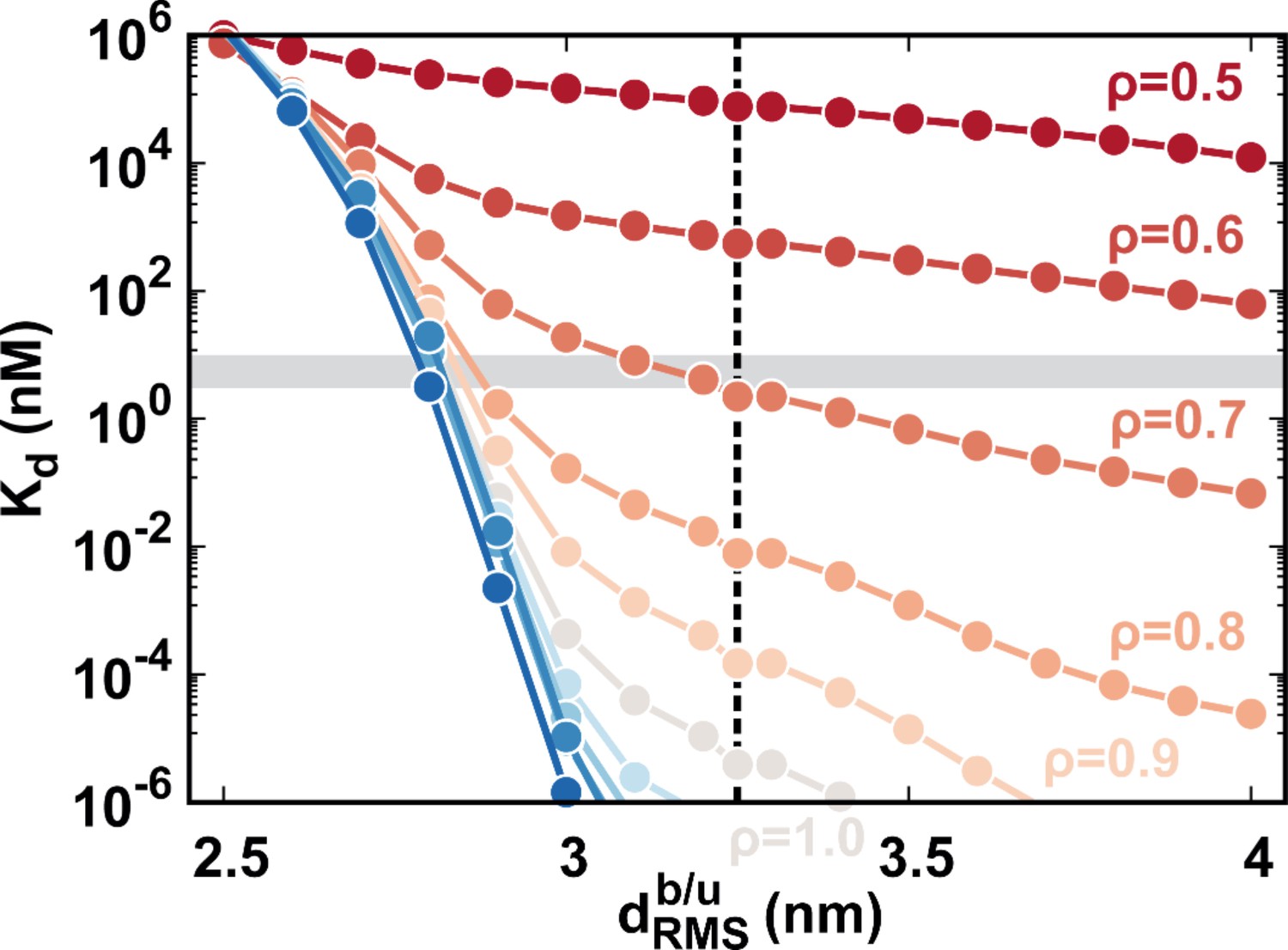
The calculated binding affinity along with at different values of .
The shadow region corresponds to the experimental binding affinity of 3–10 nM. The dashed line indicates the (3.25 nm) used in our study. The theoretical at =0.7 is equal to 2.24 nM, approximating to the experimental measurements (3–10 nM).
Appendix 3—figure 13
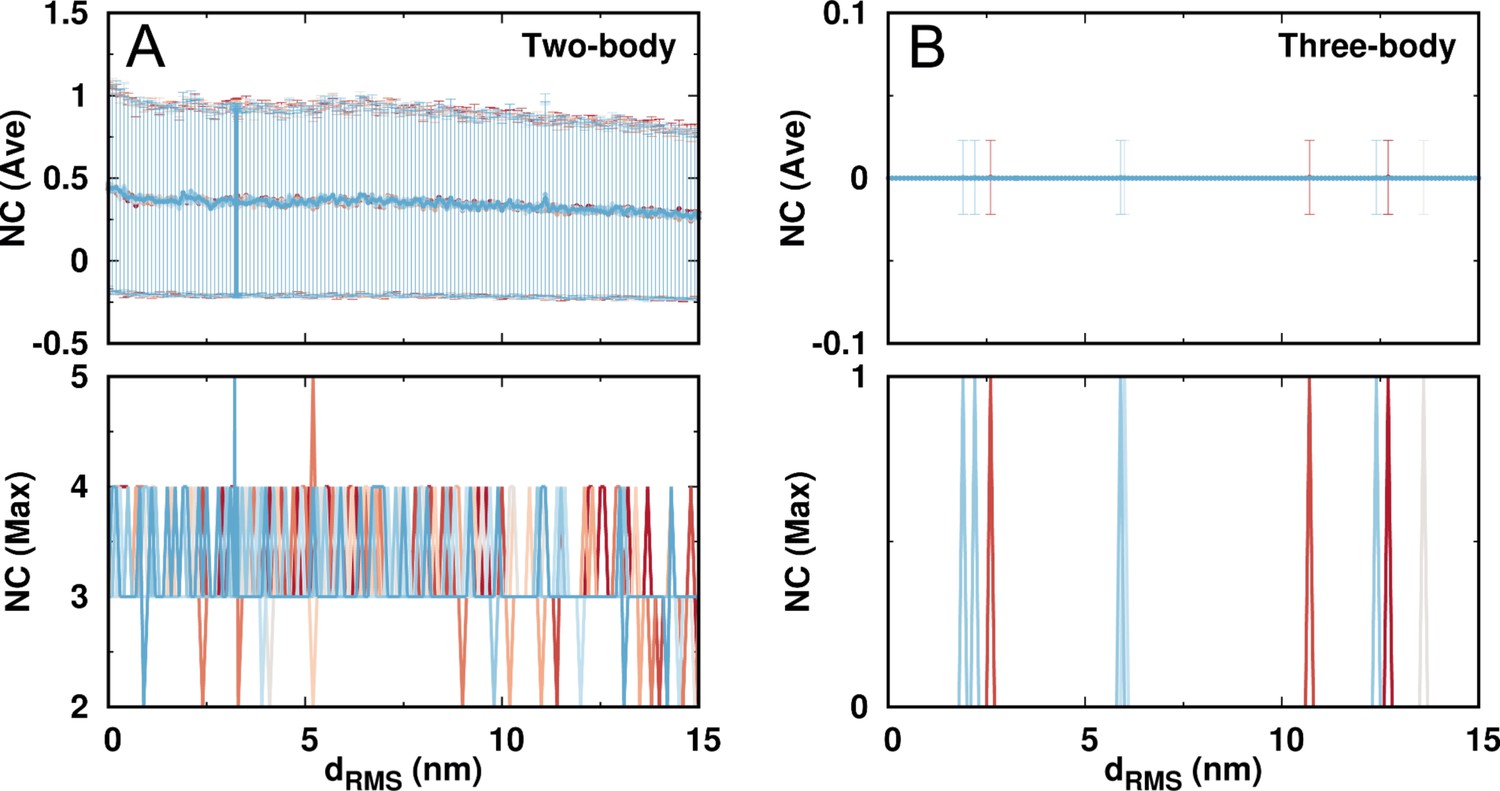
The number of contacts (NC) formed by the same charged beads in DPO4 during the DNA binding.
The contacts are further classified into the (A) two-body and (B) three-body types. A contact is considered to form when the two beads are within the range of 0.5 nm, which is the distance for the two oppositely charged beads having DH potential strength equal to the native contact strength (1.0). The two-body (pairwise) contacts can be formed with a relatively low chance indicated by both the average and maximum contact numbers. At the same time, DPO4 is almost devoid of the three-body contacts formed by the same charged residues. This features no abnormally high number of same charges accumulated in a limited spatial space.
Tables
Key resources table
| Reagent type (species) or resource | Designation | Source or reference | Identifiers | Additional information |
|---|---|---|---|---|
| Software algorithm | GROMACS(version 4.5.7) | DOI:10.1002/jcc.20291 | RRID:SCR_014565 | |
| Software, algorithm | PLUMED(version 2.5.0) | DOI:10.1016/j.cpc.2013.09.018 | https://www.plumed.org/ | |
| Software, algorithm | MATLAB | MathWorks | RRID:SCR_001622 | |
| Software, algorithm | Gnuplot(version 5.2) | http://www.gnuplot.info/ | RRID:SCR_008619 | |
| Software, algorithm | Pymol(version 1.8) | Schrdödinger,Inc | RRID:SCR_000305 |
Appendix 2—table 1
The native contact numbers of the intra- and interdomain, as well as the flexible Linker in apo-DPO4 PDB structure (PDB: 2RDI).
The total native contact number of the apo-DPO4 structure is 933, among which the intradomain native contact number is 787 and the number of interdomain native contacts that are mostly formed by the sequential neighbor domains, is 90. There are only two interdomain contacts formed by the non-sequential neighbor domains (P-LF interdomain interface). The number of contacts formed by the flexible Linker is 54. In DPO4–DNA binary PDB structure (PDB: 2RDJ), the T-LF contacts in apo-DPO4 PDB structure are fully broken and at the same time, 11 contacts are formed between the F and LF domains. These contacts are termed as the specific binary DPO4–DNA native contacts in constructing the 'double-basin’ SBM potential (). The other contacts remain the same in apo-DPO4 and binary DPO4–DNA structures.
| F domain | P domain | T domain | LF domain | Linker | |
|---|---|---|---|---|---|
| F domain | 144 | 36 | 0 | 11∗ | 0 |
| P domain | 36 | 256 | 32 | 2 | 32 |
| T domain | 0 | 32 | 130 | 22 | 9 |
| LF domain | 11∗ | 2 | 22 | 257 | 11 |
| Linker | 0 | 32 | 9 | 11 | 2 |
-
* These 11 contacts are only formed in binary DPO4–DNA structure.
Additional files
Download links
A two-part list of links to download the article, or parts of the article, in various formats.
Downloads (link to download the article as PDF)
Open citations (links to open the citations from this article in various online reference manager services)
Cite this article (links to download the citations from this article in formats compatible with various reference manager tools)
Investigating the trade-off between folding and function in a multidomain Y-family DNA polymerase
eLife 9:e60434.
https://doi.org/10.7554/eLife.60434


