Neuronal timescales are functionally dynamic and shaped by cortical microarchitecture
- Department of Cognitive Science, University of California, San Diego, United States
- Section Computational Cognitive Neuroscience, Department of Neurophysiology and Pathophysiology, University Medical Center Hamburg-Eppendorf, Germany
- Center for Brain and Cognition, Computational Neuroscience Group, Universitat Pompeu Fabra, Spain
- Halıcıoğlu Data Science Institute, University of California, San Diego, United States
- Neurosciences Graduate Program, University of California, San Diego, United States
- Kavli Institute for Brain and Mind, University of California, San Diego, United States
Figures
Figure 1
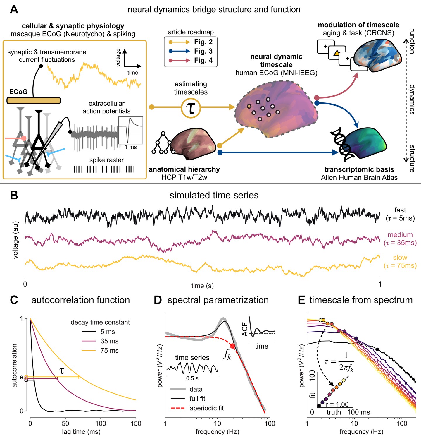
Schematic of study and timescale inference technique.
(A) In this study, we infer neuronal timescales from intracranial field potential recordings, which reflect integrated synaptic and transmembrane current fluctuations over large neural populations (Buzsáki et al., 2012). Combining multiple open-access datasets (Table 1), we link timescales to known human anatomical hierarchy, dissect its cellular and physiological basis via transcriptomic analysis, and demonstrate its functional modulation during behavior and through aging. (B) Simulated time series and their (C) autocorrelation functions (ACFs), with increasing (longer) decay time constant, τ (which neuronal timescale is defined to be). (D) Example human electrocorticography (ECoG) power spectral density (PSD) showing the aperiodic component fit (red dashed), and the ‘knee frequency’ at which power drops off (, red circle; insets: time series and ACF). (E) Estimation of timescale from PSDs of simulated time series in (B), where the knee frequency, , is converted to timescale, τ, via the embedded equation (inset: correlation between ground truth and estimated timescale values).
Figure 2 with 4 supplements
Timescale increases along the anatomical hierarchy in humans and macaques.
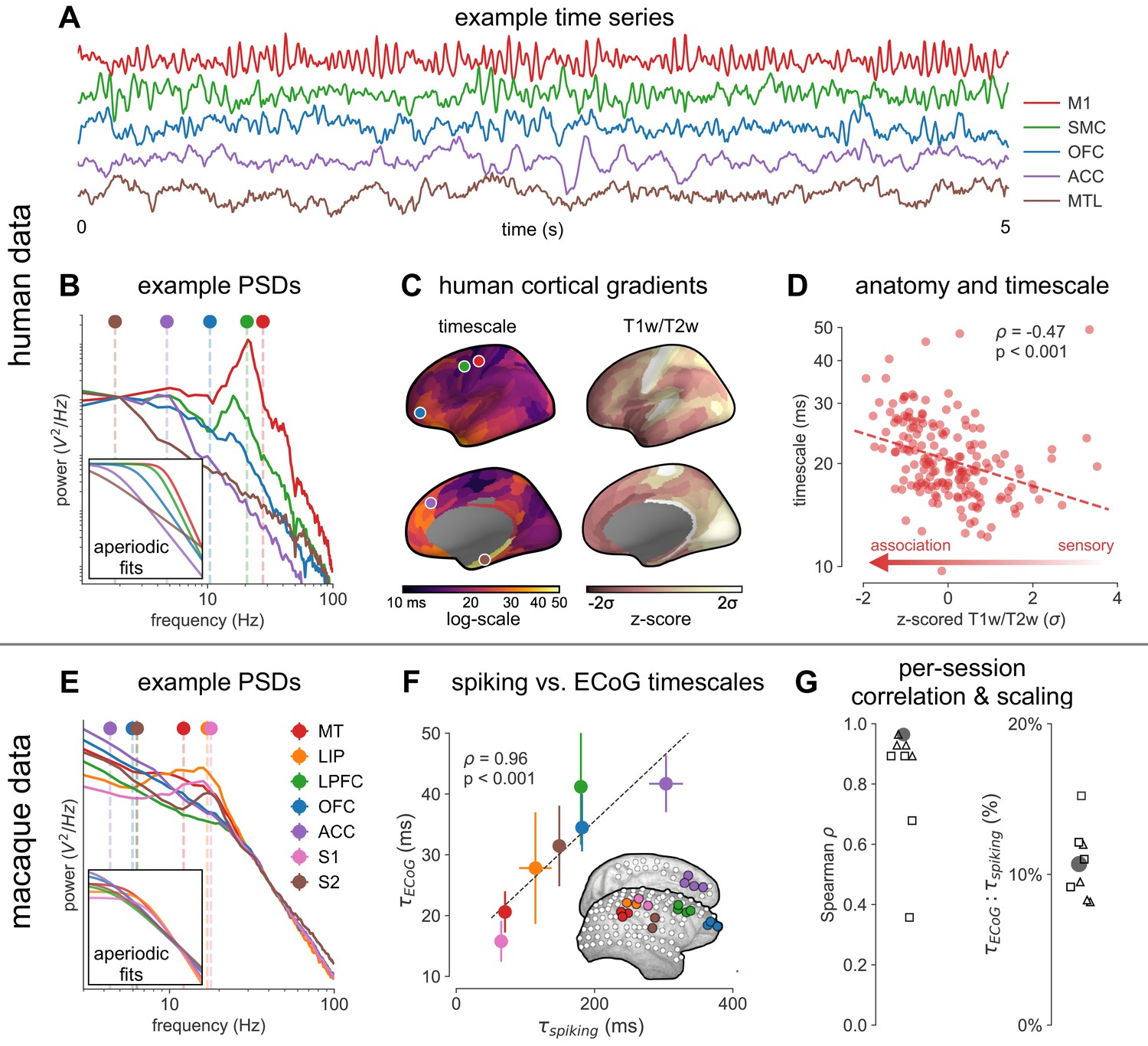
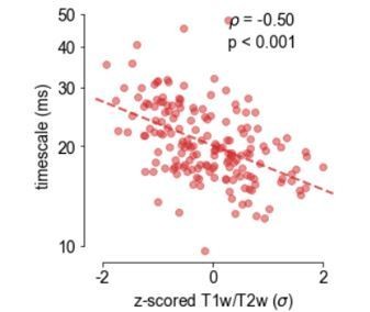
(A) Example time series from five electrodes along the human cortical hierarchy (M1: primary motor cortex; SMC: supplementary motor cortex; OFC: orbitofrontal cortex; ACC: anterior cingulate cortex; MTL: medial temporal lobe), and (B) their corresponding power spectral densities (PSDs) computed over 1 min. Circle and dashed line indicate the knee frequency for each PSD, derived from the aperiodic component fits (inset). Data: MNI-iEEG database, N = 106 participants. (C) Human cortical timescale gradient (left) falls predominantly along the rostrocaudal axis, similar to T1w/T2w ratio (right; z-scored, in units of standard deviation). Colored dots show electrode locations of example data. (D) Neuronal timescales are negatively correlated with cortical T1w/T2w, thus increasing along the anatomical hierarchy from sensory to association regions (Spearman correlation; p-value corrected for spatial autocorrelation, Figure 2—figure supplement 2A–C). (E) Example PSDs from macaque ECoG recordings, similar to (B) (LIP: lateral intraparietal cortex; LPFC: lateral prefrontal cortex; S1 and S2: primary and secondary somatosensory cortex). PSDs are averaged over electrodes within each region (inset of [F]). Data: Neurotycho, N = 8 sessions from two animals. (F) Macaque ECoG timescales track published single-unit spiking timescales (Murray et al., 2014) in corresponding regions (error bars represent mean ± s.e.m). Inset: ECoG electrode map of one animal and selected electrodes for comparison. (G) ECoG-derived timescales are consistently correlated with (left), and ~10 times faster than (right), single-unit timescales across individual sessions. Hollow markers: individual sessions; shapes: animals; solid circles: grand average from (F).
Figure 2—figure supplement 1
MNI-iEEG dataset electrode coverage.
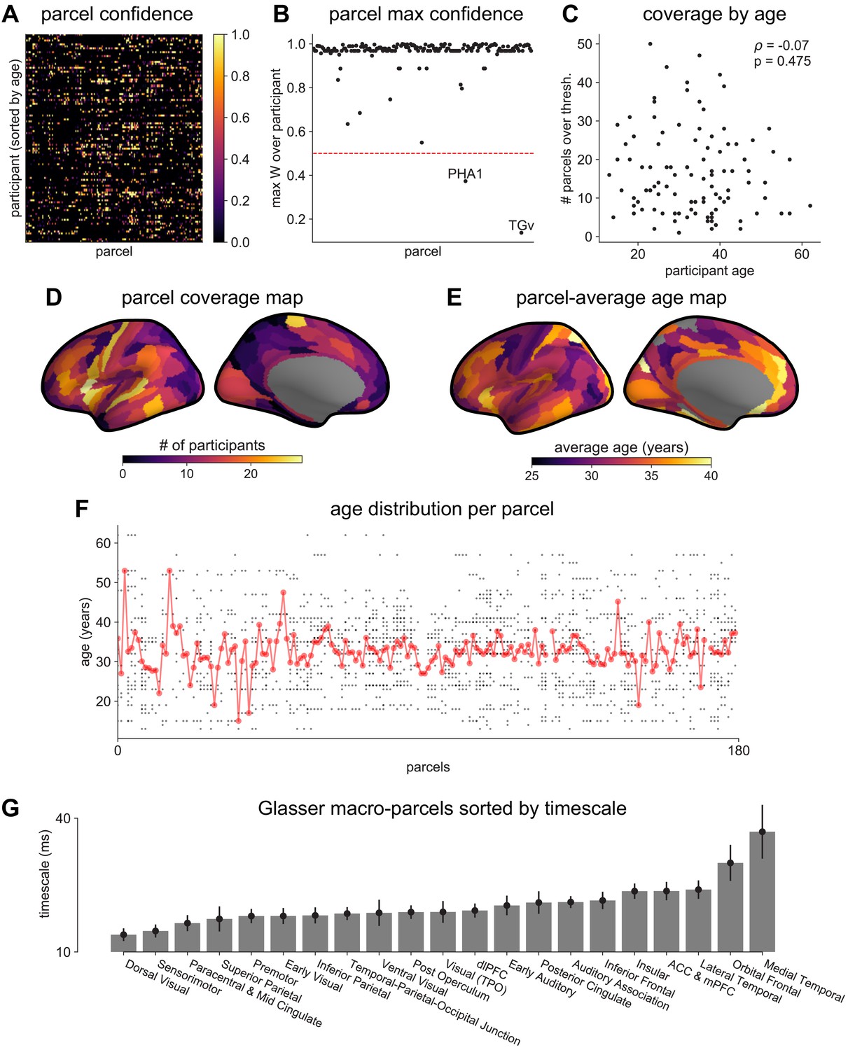
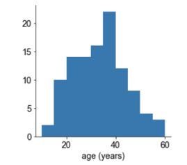
(A) Per-parcel Gaussian-weighted mask values showing how close the nearest electrode was to a given HCP-MMP1.0 parcel for each participant. Brighter means closer, 0.5 corresponds to the nearest electrode being 4 mm away. (B) Maximum mask weight for each parcel across all participants. Most parcels have electrodes very close by in at least one participant across the entire participant pool. (C) The number of valid HCP-MMP parcels each participant has above the confidence threshold of 0.5 is uncorrelated with age. (D) Cortical map of the number of participants with confidence above threshold at each parcel. Sensorimotor, frontal, and lateral temporal regions have the highest coverage. (E) Cortical map of the average age of participants with confidence above threshold at each parcel. (F) Age distribution of participants with confidence above threshold at each parcel. Average age per parcel (red line) is relatively stable while age distribution varies from parcel to parcel (each subject is a black dot). (G) Average neuronal timescale when further aggregating the 180 Glasser parcels into 21 macro-regions (mean ± s.e.m across parcels within the macro-region).
Figure 2—figure supplement 2
Comparison of spatial autocorrelation-preserving null map generation methods.
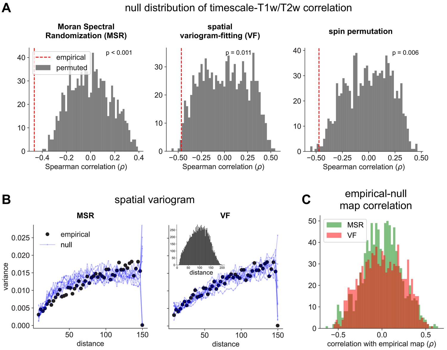
(A) Distributions of Spearman correlation values between empirical T1w/T2w map and 1000 spatial-autocorrelation preserving null timescale maps generated using Moran Spectral Randomization (MSR), spatial variogram fitting (VF), and spin permutation. Red dashed line denotes correlation between empirical timescale and T1w/T2w maps, p-values indicate two-tailed significance, i.e., proportion of distribution with values more extreme than empirical correlation. (B) Spatial variogram for empirical timescale map (black) and 10 null maps (blue) generated using MSR (left) and VF (right). Inset shows distribution of distances between pairs of HCP-MMP parcels. (C) Distribution of Spearman correlations between empirical and 1000 null timescale maps generated using MSR (green) and VF (red), showing similar levels of correlation between empirical and null maps for both methods.
Figure 2—figure supplement 3
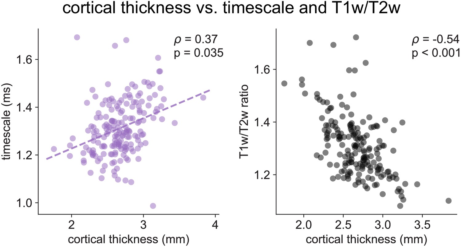
Cortical thickness.
Cortical thickness from the HCP dataset is positively correlated with neuronal timescale (left) and negatively correlated with T1w/T2w, i.e., thicker brain regions have longer (slower) timescales and less gray matter myelination, corresponding to higher-order association areas.
Figure 2—figure supplement 4

Macaque ECoG and single-unit coverage.
(A) Locations of 180-electrode ECoG grid from two animals in the Neurotycho dataset; colors correspond to locations used for comparison with single-unit timescales. (B) Electrode indices of the sampled areas from the two animals, corresponding to those colored in (A).
Figure 3 with 2 supplements
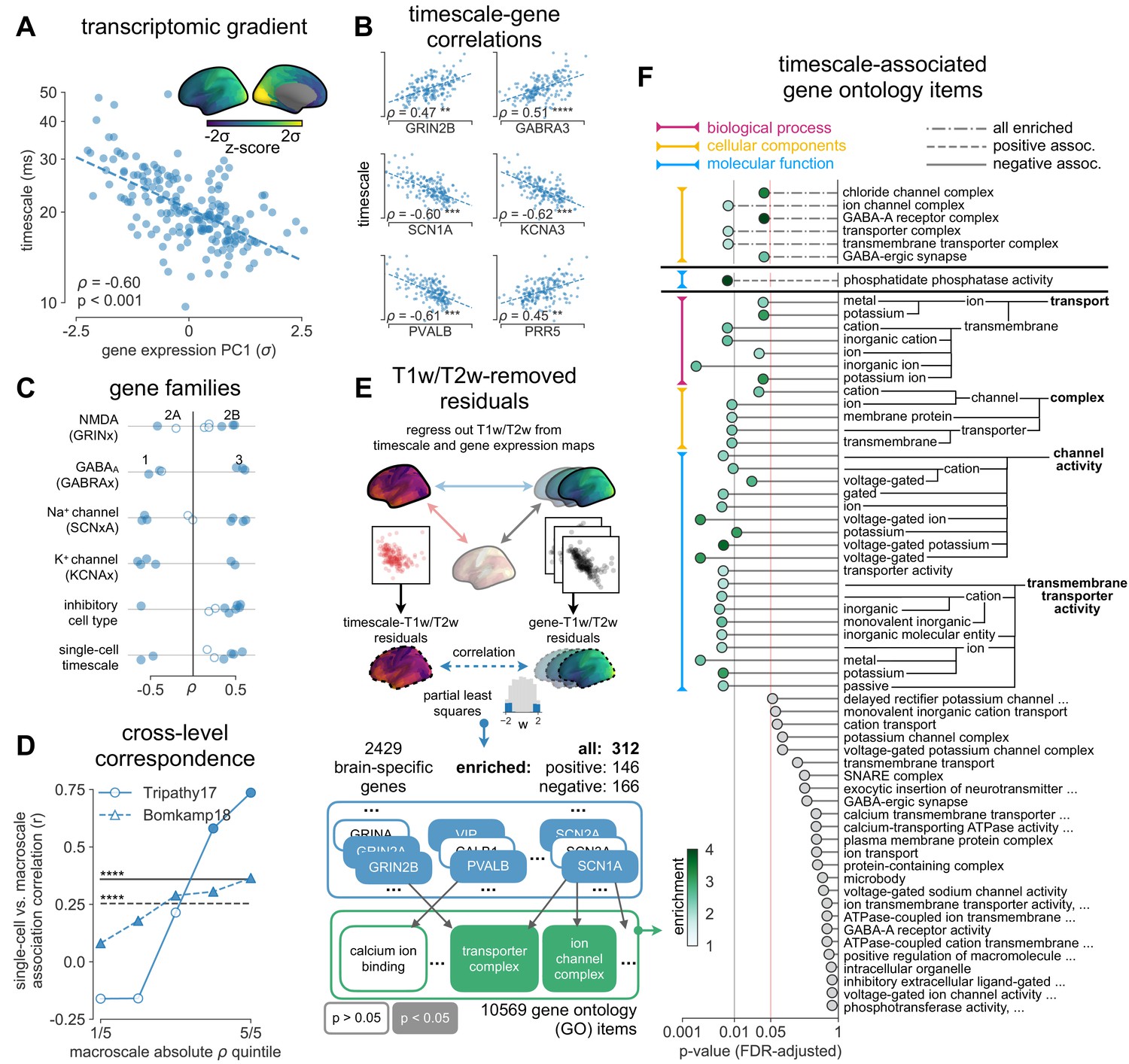
Timescale gradient is linked to expression of genes related to synaptic receptors and transmembrane ion channels across the human cortex.
(A) Timescale gradient follows the dominant axis of gene expression variation across the cortex (z-scored PC1 of 2429 brain-specific genes, arbitrary direction). (B) Timescale gradient is significantly correlated with expression of genes known to alter synaptic and neuronal membrane time constants, as well as inhibitory cell-type markers, but (C) members within a gene family (e.g., NMDA receptor subunits) can be both positively and negatively associated with timescales, consistent with predictions from in vitro studies. (D) Macroscale timescale-transcriptomic correlation captures association between RNA-sequenced expression of the same genes and single-cell timescale properties fit to patch clamp data from two studies, and the correspondence improves for genes (separated by quintiles) that are more strongly correlated with timescale (solid: N = 170 [Tripathy et al., 2017], dashed: N = 4168 genes [Bomkamp et al., 2019]; horizontal lines: correlation across all genes from the two studies, ρ = 0.36 and 0.25, p<0.001 for both). (E) T1w/T2w gradient is regressed out from timescale and gene expression gradients, and a partial least squares (PLS) model is fit to the residual maps. Genes with significant PLS weights (filled blue boxes) compared to spatial autocorrelation (SA)-preserved null distributions are submitted for gene ontology enrichment analysis (GOEA), returning a set of significant GO terms that represent functional gene clusters (filled green boxes). (F) Enriched genes are primarily linked to potassium and chloride transmembrane transporters, and GABA-ergic synapses; genes specifically with strong negative associations further over-represent transmembrane ion exchange mechanisms, especially voltage-gated potassium and cation transporters. Branches indicate GO items that share higher-level (parent) items, e.g., voltage-gated cation channel activity is a child of cation channel activity in the molecular functions (MF) ontology, and both are significantly associated with timescale. Color of lines indicate curated ontology (BP—biological process, CC—cellular components, or MF). Dotted, dashed, and solid lines correspond to analysis performed using all genes or only those with positive or negative PLS weights. Spatial correlation p-values in (A–C) are corrected for SA (see Materials and methods; asterisks in (B,D) indicate p<0.05, 0.01, 0.005, and 0.001 respectively; filled markers in (C,D) indicate p<0.05).
Figure 3—figure supplement 1
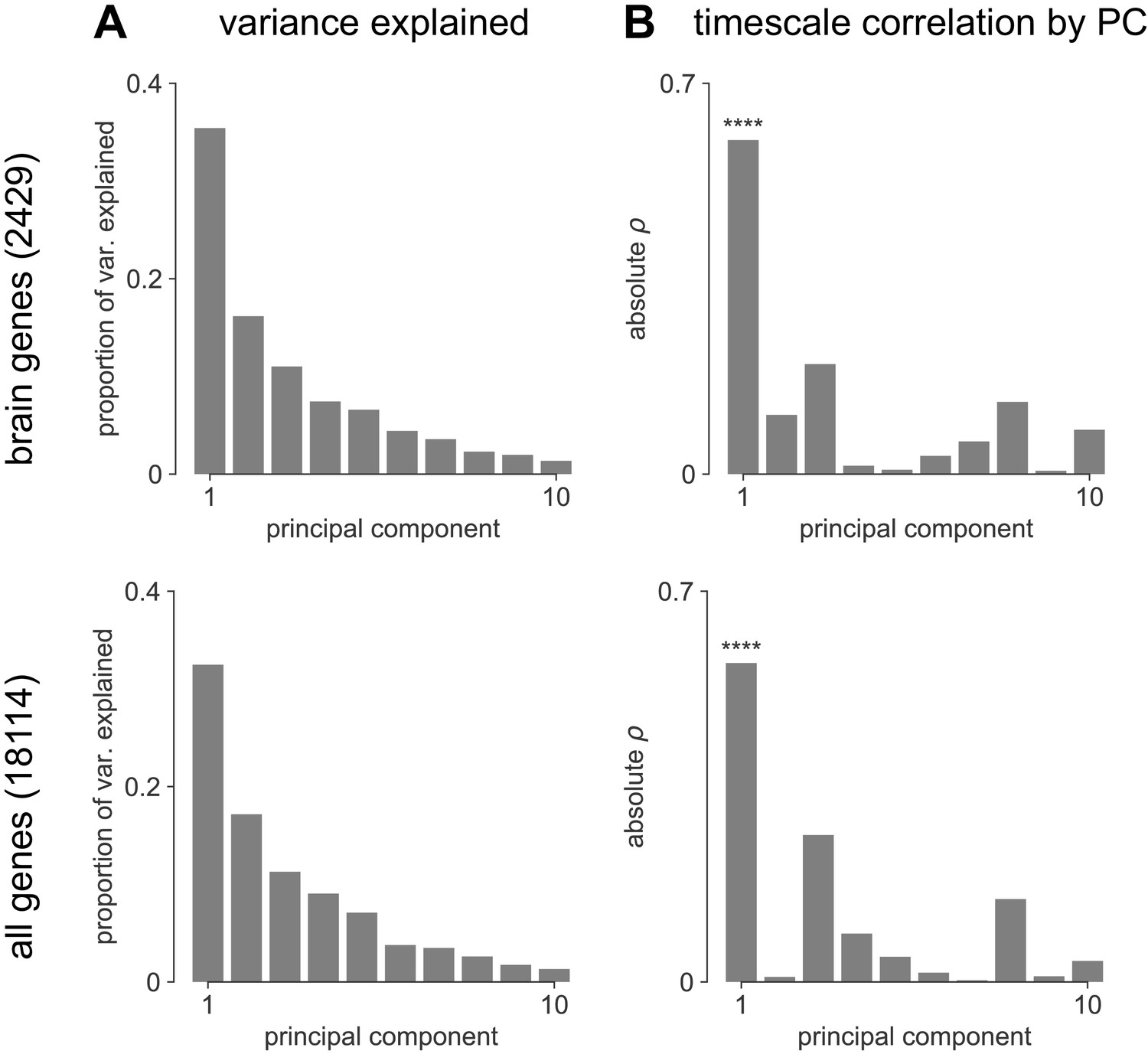
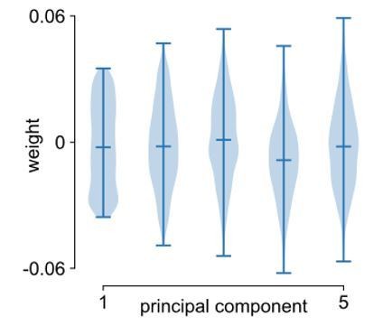
Transcriptomic principal component analysis results.
(A) Proportion of variance explained by the top 10 principal components (PCs) of brain-specific genes (top) and all AHBA genes (bottom). (B) Absolute Spearman correlation between timescale map and top 10 PCs from brain-specific or full gene dataset. Asterisks indicate resampled significance while accounting for spatial autocorrelation; **** indicate p<0.001. Top PCs explain similar amounts of variance, while only PC1 in both cases is significantly correlated with timescale.
Figure 3—figure supplement 2

Individual timescale-gene correlations magnitudes.
Correlation between timescale and expression of genes from Figure 3C, with gene symbols labeled and grouped into functional families for ease of interpretation.
Figure 4 with 2 supplements
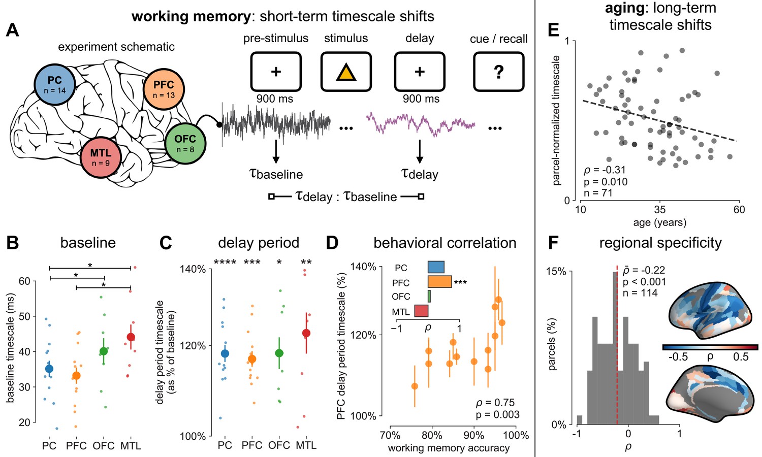
Timescales expand during working memory maintenance while tracking performance, and task-free average timescales compress in older adults.
(A) Fourteen participants with overlapping intracranial coverage performed a visuospatial working memory task, with 900 ms of baseline (pre-stimulus) and delay period data analyzed (PC: parietal, PFC: prefrontal, OFC: orbitofrontal, MTL: medial temporal lobe; n denotes number of subjects with electrodes in that region). (B) Baseline timescales follow hierarchical organization within association regions (*: p<0.05, Mann–Whitney U-test; small dots represent individual participants, large dots and error bar for mean ± s.e.m. across participants). (C) All regions show significant timescale increase during delay period compared to baseline (asterisks represent p<0.05, 0.01, 0.005, 0.001, Wilcoxon signed-rank test). (D) PFC timescale expansion during delay periods predicts average working memory accuracy across participants (dot represents individual participants, mean ± s.e.m. across PFC electrodes within participant); inset: correlation between working memory accuracy and timescale change for all regions. (E) In the MNI-iEEG dataset, participant-average cortical timescales decrease (become faster) with age (n = 71 participants with at least 10 valid parcels, see Figure 4—figure supplement 2B). (F) Most cortical parcels show a negative relationship between timescales and age, with the exception being parts of the visual cortex and the temporal poles (one-sample t-test, t = −7.04, p<0.001; n = 114 parcels where at least six participants have data, see Figure 4—figure supplement 2C).
Figure 4—figure supplement 1
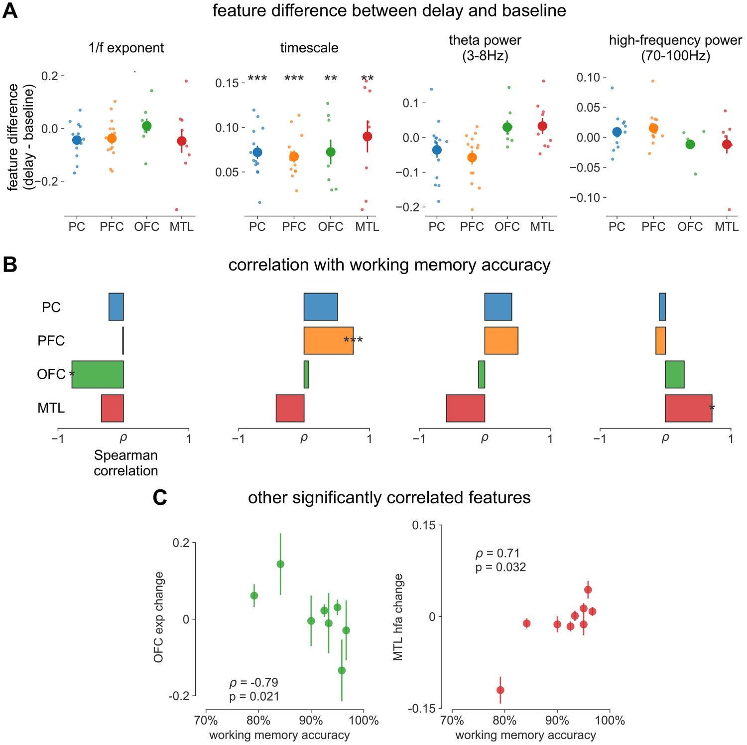
Spectral correlates of working memory performance.
(A) Difference between delay and baseline periods for 1/f-exponent, timescale (same as main Figure 4C but absolute units on y-axis, instead of percentage), theta power, and high-frequency power. (B) Spearman correlation between spectral feature difference and working memory accuracy across participants, same features as in (A). *p<0.05, **p<0.01, ***p<0.005 in (A, B). (C) Scatter plot of other significantly correlated spectral features from (B).
Figure 4—figure supplement 2
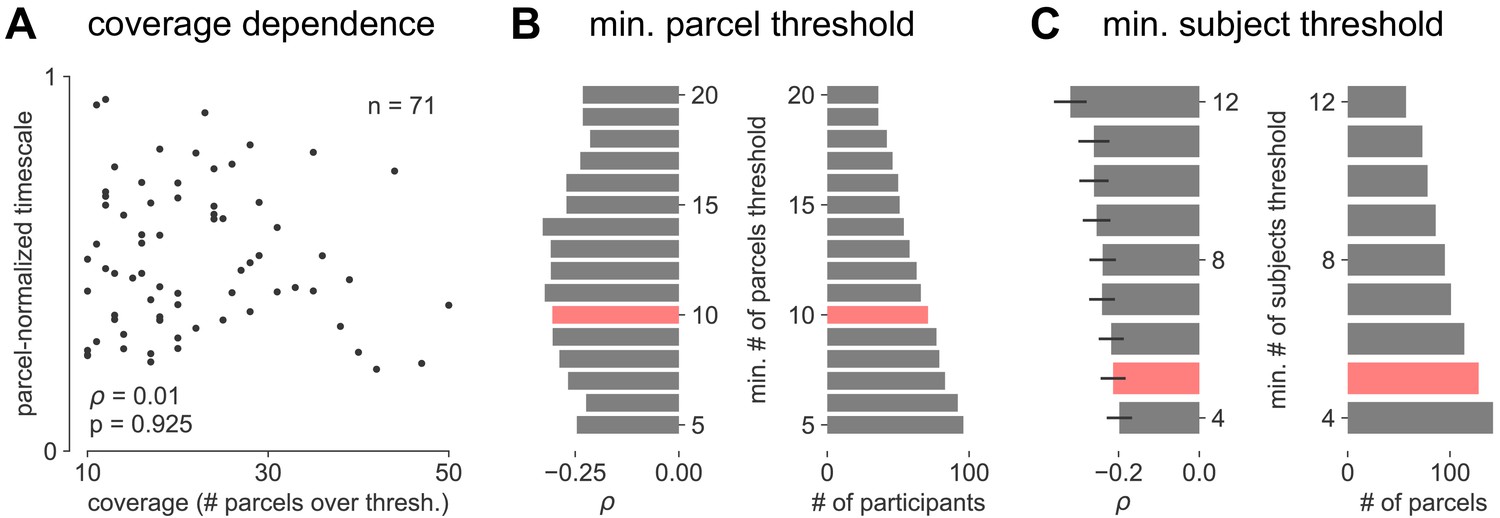
Parameter sensitivity for timescale-aging analysis.
(A) Cortex-averaged timescale is independent of parcel coverage across participants. (B) Sensitivity analysis for the number of valid parcels a participant must have in order to be included in analysis for main Figure 4E (red). As threshold increases (more stringent), fewer participants satisfy the criteria (right) but correlation between participant age and timescale remains robust (left). (C) Sensitivity analysis for the number of valid participants a parcel must have in order to be included in analysis for main Figure 4F. As threshold increases (more stringent), fewer parcels satisfy the criteria (right) but average correlation across all parcels remains robust (left, error bars denote s.e.m of distribution as in Figure 4F).
Author response image 1
Author response image 2
Author response image 3
Tables
Table 1
Summary of open-access datasets used.
| Data | Ref. | Specific source/format used | Participant info | Relevant figures |
|---|---|---|---|---|
| MNI Open iEEG Atlas | Frauscher et al., 2018a; Frauscher et al., 2018b | N = 105 (48 females) Ages: 13–65, 33.4 ± 10.6 | Figure 2A–D, Figure 3, Figure 4E and F | |
| T1w/T2w and cortical thickness maps from Human Connectome Project | Glasser et al., 2016; Glasser and Van Essen, 2011 | Release S1200, March 1, 2017 | N = 1096 (596 females) Age: 22–36+ (details restricted due to identifiability) | Figure 2C and D, Figure 3D–F |
| Neurotycho macaque ECoG | Nagasaka et al., 2011; Yanagawa et al., 2013 | Eyes-open state from anesthesia datasets (propofol and ketamine) | Two animals (Chibi and George) four sessions each | Figure 2E–G |
| Macaque single-unit timescales | Murray et al., 2014 | Figure 1 of reference | Figure 2E–G | |
| Whole-cortex interpolated Allen Brain Atlas human gene expression | Gryglewski et al., 2018; Hawrylycz et al., 2012 | Interpolated maps downloadable from http://www.meduniwien.ac.at/neuroimaging/mRNA.html | N = 6 (one female) Age: 24, 31, 39, 49, 55, 57 (42.5 ± 12.2) | Figure 3 |
| Single-cell timescale-related genes | Bomkamp et al., 2019; Tripathy et al., 2017 | Table S3 from Tripathy et al., 2017, Online Table 1 from Bomkamp et al., 2019 | N = 170 (Tripathy et al., 2017) and 4168 (Bomkamp et al., 2019) genes | Figure 3C and D |
| Human working memory ECoG | Johnson, 2019; Johnson, 2018c; Johnson et al., 2018a, Johnson et al., 2018b | CRCNS fcx-2 and fcx-3 | N = 14 (five females) Age: 22–50, 30.9 ± 7.8 | Figure 4A–D |
Table 2
Reproducing figures from code repository.
| All IPython notebooks (Gao, 2020): https://github.com/rdgao/field-echos/tree/master/notebooks | |
|---|---|
| Notebook | Results |
| 1_sim_method_schematic.ipynb | Simulations: Figure 1B–E |
| 2_viz_NeuroTycho-SU.ipynb | Macaque timescales: Figure 2E–G, Figure 2—figure supplement 4 |
| 3_viz_human_structural.ipynb | Human timescales vs. T1w/T2w and gene expression: Figure 2A–D, Figure 2—figure supplements 1 and 3, Figure 3, Figure 3—figure supplements 1 and 2, Supplementary file 1–, Supplementary file 2, Supplementary file 3. |
| 4b_viz_human_wm.ipynb | Human working memory: Figure 4A–D, Figure 4—figure supplement 1 |
| 4a_viz_human_aging.ipynb | Human aging: Figure 4E and F, Figure 4—figure supplement 2 |
| supp_spatialautocorr.ipynb | Spatial autocorrelation-preserving nulls: |
| supp_spatialautocorr.ipynb | Spatial autocorrelation-preserving nulls: Figure 2—figure supplement 2 |
Additional files
-
Supplementary file 1
Significant items from brain-specific GOEA (data for Figure 3F).
- https://cdn.elifesciences.org/articles/61277/elife-61277-supp1-v2.docx
-
Supplementary file 2
Significant items from all-gene GOEA.
- https://cdn.elifesciences.org/articles/61277/elife-61277-supp2-v2.docx
-
Supplementary file 3
Significant items from all-gene GOEA with T1w/T2w as control.
- https://cdn.elifesciences.org/articles/61277/elife-61277-supp3-v2.docx
-
Transparent reporting form
- https://cdn.elifesciences.org/articles/61277/elife-61277-transrepform-v2.pdf
Download links
A two-part list of links to download the article, or parts of the article, in various formats.
Downloads (link to download the article as PDF and Executable version)
Open citations (links to open the citations from this article in various online reference manager services)
Cite this article (links to download the citations from this article in formats compatible with various reference manager tools)
Neuronal timescales are functionally dynamic and shaped by cortical microarchitecture
eLife 9:e61277.
https://doi.org/10.7554/eLife.61277


