A small, computationally flexible network produces the phenotypic diversity of song recognition in crickets
Figures
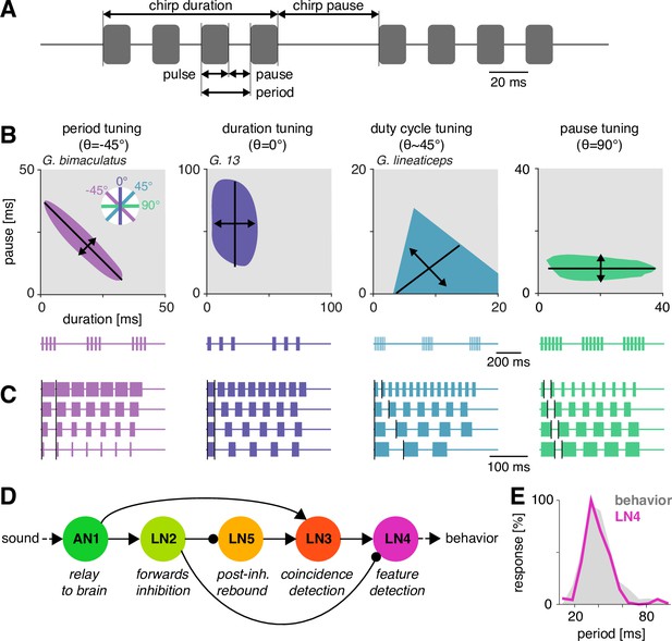
Song structure and song preference in crickets, and the song recognition network of Gryllus bimaculatus.
(A) Parameters of the temporal pattern of cricket song. Short sound pulses are interleaved by pulse pauses. The pulse period is given by the sum of pulse duration and pulse pause. The pulse duty cycle corresponds to signal energy and is given by the ratio between pulse duration and period. In many species, pulses are grouped in chirps and interleaved by a chirp pause, while other species produce continuous pulse trains, called trills. (B) The behavioral tuning for pulse patterns can be characterized using response fields, which mark the set of behaviorally preferred pulse parameters in a two-dimensional diagram spanned by pulse duration and pause duration. Shown are schematics derived from behavioral data from particular species illustrating the four principal response types known from crickets and other insects. Traces below each response field show typical song patterns for each species. Response types can be defined based on tolerance (black lines) and selectivity (double headed arrows) for particular stimulus parameters, leading to specific orientations of the response field (see left inset): period tuning (purple, G. bimaculatus) is defined by selectivity for pulse period and tolerance for pulse duty cycle, giving an orientation of the response field of –45°. Duration tuning (lilac, G13, Gray et al., 2016) leads to vertically oriented response fields. Duty cycle tuning (cyan, Gryllus lineaticeps, Hennig et al., 2016) leads to diagonally oriented response fields. Pause tuning (green) with horizontal response fields is not known from crickets but has been reported in the katydid Tettigonia viridissima (Schul, 1998). The response field given represents a hypothetical cricket species. (C) Example stimulus series illustrating the stimulus features each response type in (B) is selective for. Vertical black lines mark the feature that is constant for each stimulus series. For duty cycle (cyan), the ratio between pulse duration and period is constant. (D) Song recognition network in the brain of G. bimaculatus. The network consists of five neurons, each with a specific computational role, which are connected in a feed-forward manner using excitation (pointed arrowheads) and inhibition (round arrowheads). The excitatory ascending neuron 1 (AN1) relays information from auditory receptors in the prothorax to the brain. The inhibitory local neuron 2 (LN2) inverts the sign of forwarded responses. LN2 inhibits the non-spiking LN5 neuron, which produces a post-inhibitory rebound. LN3 acts as a coincidence detector for excitatory input from AN1 and LN5. Input delays are tuned such that LN3 is maximally driven by the conspecific pulse train with a pulse period of 30–40 ms. LN4 integrates excitatory input from LN3 and inhibitory input from LN2 and further sharpens the output of the network. (E) Tuning for pulse period in LN4 (purple) matches the phonotactic behavior (gray) of G. bimaculatus females (D, E adapted from Figures 5A and 6A; Schöneich et al., 2015).
© 2015, Schöneich et al. Figure 1D & E are adapted E Tuning for pulse period in LN4 (purple) matches the phonotactic behavior (gray) of G. bimaculatus females (D, E adapted from Figures 5A and 6A, Schöneich et al., 2015).
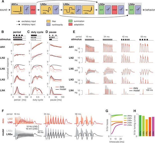
A computational model reproduces the responses of the song recognition network.
(A) The model of the song recognition network (Figure 1D) combines four elementary computations: linear filtering (yellow), static nonlinearities (blue), adaptation (red), and synaptic transmission (black lines, pointed arrowheads: excitatory inputs; round arrowheads: inhibitory inputs). Multiple inputs to a cell are summed (green). Pictograms inside of each box depict the shapes of the filters and of the nonlinearities. Y scales are omitted for clarity. See Figure 2—figure supplement 1, Figure 2—figure supplement 2, and Materials and methods for details. (B–D) Tuning for period (B), duty cycle (C), and pause (D) in the data (red, each line is a trial-averaged recording from one individual) and in the model (black) for the five neurons in the network. Thicker red lines depict the recording used for fitting. Stimulus schematics are shown on the top of each plot. Tuning is given by the firing rate (AN1, LN2–4) or integral rebound voltage (LN5) for each chirp and was normalized to peak at 1.0 across the whole set of tuning curves shown in (B–D). A duration tuning curve is not shown since it is not contained in the electrophysiological data. See Figure 3 for duration tuning generated by the model. Number of individual recordings is 8/4/3/6/4 for AN1/LN2/5/3/4. (E) Firing rate (Hz) or membrane voltage (mV) traces from the recording used for fitting (red) and from the model (black). Stimuli (top) are pulse trains with different pulse periods. (F) Firing rate of LN2 in Hz (shaded area) and membrane voltage traces of LN5 in mV (line) in the recording used for fitting (top, red) and in the model (bottom, black) for short (18 ms), intermediate (34 ms), and long (58 ms) periods. The model reproduces the response timing of LN5 and LN2 responses overlap for short and intermediate but not for long periods. (G) Goodness of fit for the response dynamics of all neurons at different timescales, quantified as the between the traces in the data and the model. Fits for AN1M, LN2M, and LN5M are good across all timescales. The fits for LN3M and in particular for LN4M increase with timescale (>10 ms) due to the sparse and variable spiking of these neurons (see E). (H) Goodness of fit for the tuning curves, quantified as 1 minus the root mean-square error between the tuning curves from the data and the model (compare black lines and thick red lines in B–D). The curves from the data and the model were normalized by the peak of the curve from the data, to make the measure independent of response scale. Performance is high for all neurons. The weaker match for LN5M stems from larger model responses for stimuli with long periods or pauses (see B, D).
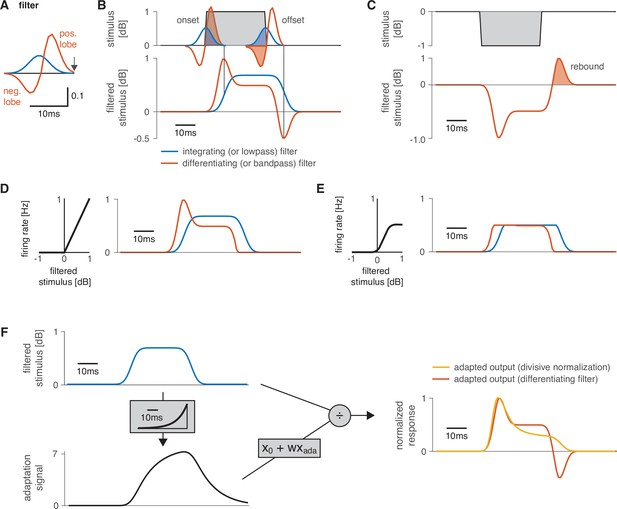
Working principle of filters and nonlinearities used as building blocks in the model.
(A) Shapes of a low-pass or integrating filter (blue) and of a bandpass or differentiating filter (orange). Filters are unitless. The integrating filter was generated from a Gaussian, and the differentiating filter was obtained by taking the derivative of the integrating filter and scaling the negative filter lobe by ½. A neuron’s filter depicts the stimulus pattern that strongly drives that neuron. The output is generated at the right end of the filter (arrow). (B) Output of the two filters in (A) for a square pulse (top). The filtered stimulus (bottom) is generated by sliding the filter over the stimulus and computing the sum over the pointwise product between the filter shape and the stimulus. The filtered stimulus is produced at the right end of the filter (vertical lines). The integrating filter (blue) smooths the sharp on- and offsets of the pulse. The differentiating filter is a change detector because it responds strongly to changes in the stimulus (orange): a strong positive response occurs at pulse onset because only the excitatory lobe is ‘activated’ by the stimulus (‘activation’ indicated by the shaded part of the filters on top). A negative response at pulse offset arises because only the negative filter lobe overlaps with the pulse. An intermediate response is produced during the pulse because the excitatory lobe is 2× larger than the inhibitory lobe. A fully symmetrical filter would produce no response for constant stimuli irrespective of the stimulus amplitude. A differentiating filter produces a phasic-tonic response pattern and is therefore useful for reproducing adapting responses in AN1M, LN2M, or the inputs in LN5M (Figure 2—figure supplement 2). (C) The rebound responses of LN5M were reproduced with a differentiating filter. The response (bottom, dashed orange line) of the differentiating filter in (A) to a negative input (top) equals the sign-inverted response of that filter to a positive input (compare B). The positive response of a differentiating filter for pulse offsets (shaded area) reproduces the post-inhibitory rebound response of the LN5 neuron (Figure 2—figure supplement 2). (D) A rectifying nonlinearity (left) and the output of the nonlinearity (right) for the stimulus filtered with a low- and a bandpass filter from (B). The nonlinearity with a threshold value of 0 cuts off all negative filter outputs. (E) A sigmoidal nonlinearity (left) and the output for the filtered stimulus (right) for both filters from (B). This nonlinearity cuts off small and compresses large filter outputs. In the example, it compresses the onset accentuation and cuts off the negative offset response for the differentiating filter (orange). The responses for the differentiating (orange) and the integrating (blue) filter now mainly differ in their delay, with the differentiating filter leading the integrating filter because the peak of the differentiating filter occurs closer to the time of the response (arrow in A). (F) Divisive normalization acts by scaling its input (from top left, blue, to yellow, right). The input (top left, blue) is filtered by an adaptation filter to produce the adaptation signal (middle left, black), which is linearly transformed to divide the input . For this example, the adaptation filter (gray box on the left) of the divisive normalization stage was an exponential kernel with a width =40 ms, was scaled to peak at 1, and has units 1 /dB. The orange trace shows the output of the differentiating filter from (A). The responses in the right panel were normalized to peak at 1.0 to facilitate comparison of their time courses.

Illustration of the model parameters.
The model combines four elementary computations: filtering (yellow boxes), adaptation (red boxes), nonlinear transfer functions (blue boxes), and delayed transmission (black lines, pointed arrowheads: excitatory inputs; round arrowheads: inhibitory inputs). Summation of synaptic inputs is marked with green boxes. The graphs in the yellow boxes show the filters, x-axis is time. The postsynaptic filter for LN5M is very short 3 ms ( = 3 time steps in the model) – the step-like pattern arises because of the discrete time steps at which the filters are presented; individual plateaus correspond to individual time steps in the filter. The graphs in the blue boxes show the nonlinearities, x-axis is the input, y-axis is the output activation. The adaptation stage has three parameters: speed, strength, and offset. The filters shown in the red boxes correspond to the exponential filters that generate the adaptation signal that is used to divide the filtered stimulus (see Figure 1G). The exponential filter for the adaptation stage in AN1M does not reach baseline because it is truncated in the model. The inhibitory lobe of the AN1M filter is used to implement adaptation and is enlarged in the plot for clarity. See Table 1 for all parameter values and Figure 2—figure supplement 1 for an illustration of the working principles of the filters, nonlinearities, and delayed transmission.

Goodness of fit for the response dynamics for each neuron in the network model, separated by stimulus.
Firing rate or voltage rate (for the non-spiking LN5) of each recording used for fitting (red) and goodness of fit () at timescales 1, 12, and 24 ms (gray lines; compare Figure 2G). The at different timescales was obtained by low-pass filtering the firing rate traces from the experimental data and the model with a box filter of the respective duration. The is largely independent of stimulus and timescale for AN1, LN2, LN5, and LN3, which produce dense spiking or voltage responses. Low values in LN4 arise at short timescales and for stimuli that elicit very few and irregularly timed spikes.

LN4M response fields for different amplitudes of the LN5M rebound.
Rebound amplitude is given relative to the value in the original model (1.0). Halving or doubling the amplitude has minor impacts on the model responses.

Model responses to novel pulse train stimuli.
Responses of the model neurons for stimuli with different combinations of pulse and pause durations (1–80 ms, 1600 stimuli per response field, color code corresponds to response magnitude). Each response field depicts the firing rate (for AN1M, LN2M–4M) or the voltage of the rebound (for LN5M) of model neurons. Pulse trains had a fixed duration of 140 ms and were interleaved by a pause of 200 ms, mimicking the chirp structure of G. bimaculatus calling song. Anti-diagonal step-like patterns in the response fields arise from changes in the number of pulses per train (Figure 3—figure supplement 1A and B). Although the data set used for fitting did not include stimuli with long pulse durations, the model predicts the weak response known from the behavior for these stimuli. Solid black lines indicate stimuli with 15 ms pause duration (horizontal), 15 ms pulse duration (vertical), 30 ms pulse period (anti-diagonal), and 0.5 pulse duty cycle (diagonal). Dots in the leftmost panel mark the stimuli used for fitting.
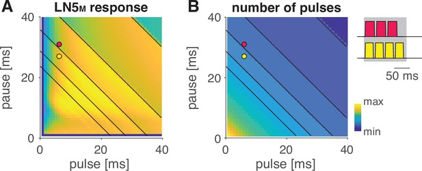
Stepwise changes in the response fields arise from the stimulus structure.
Response field of LN5M (A) and number of pulses per train in the underlying stimuli (B) (see color bar for color coding, color map was scaled to span the range of response values [A] and pulse numbers [B]). Changes in pulse number are marked by anti-diagonal black lines in both panels (only shown for pulse duration and pauses greater than 20 ms for clarity). Red and yellow dots in the fields in (A) and (B) refer to the two pulse train stimuli shown on the right of (B) with three pulses (red) and four pulses (yellow), and the maximal pulse train duration of 140 ms is shown as a gray shaded area. Steps in the response fields (A, Figure 3) arise from stepwise changes in the number of pulses per train (B) due to the fixed pulse train duration.
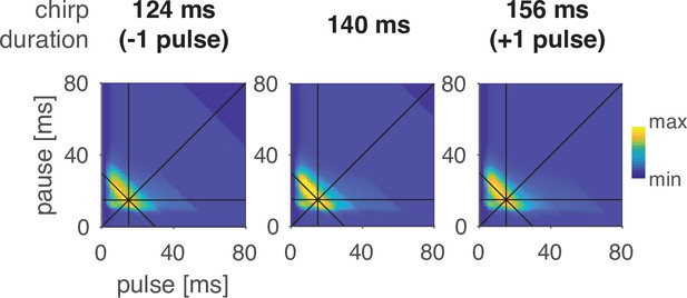
Preference for pulse parameters is robust to small changes in chirp duration.
Response fields of LN4M for pulse trains with different chirp durations and a fixed chirp pause of 200 ms. The response fields are robust to the addition or removal of a pulse from the chirp.
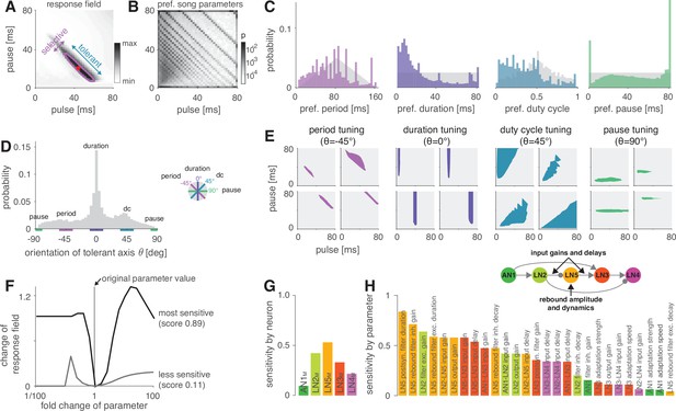
The network generates the diversity of response profiles known from crickets and other insects.
(A) Response field generated from a model variant with randomized parameters. Response magnitude coded in gray colors (see color bar). Tuning was characterized in terms of the preferred pulse and pause durations (red dot) and as tolerant (blue) or selective (purple) directions in the stimulus field. This example is period tuned (purple contour marks the 75% response level) and the set of preferred stimuli is oriented at –45° (see inset in D for a definition of the angles), corresponding to selectivity for period (purple) and tolerance for duty cycle (cyan). (B) Distribution of preferred pulse and pause parameters for all model variants generated from randomized parameter combinations (coded in gray colors, see color bar). Anti-diagonal patterns arise from the discrete nature of pulse trains (Figure 3—figure supplement 1A and B). Models that prefer pauses of 0 ms correspond to models that prefer constant tones. Enrichment of models that prefer the maximally tested pause of 80 ms indicates that the network can generate preference for longer pauses than tested. Preferences cover the stimulus field. (C) Distribution of preferred pulse parameters (left to right: pulse period, pulse duration, duty cycle, and pause). Gray histograms correspond to the distributions expected from uniform sampling of stimulus space – deviations from this distribution indicate response biases. The network is biased to produce preferences for short pulse periods, short pulse durations, and low duty cycles. Peaks in the histograms arise from the discrete nature of pulse trains (Figure 3—figure supplement 1A and B) or from boundary effects (see B). (D) Distribution of the orientation of the response fields (see A) for model variants that are well fitted by an ellipsoid, have a single peak, and are asymmetrical. Colored lines indicate the range of angles (±10°) that correspond to the four principal response types (see inset and Figure 1B). The network can produce response fields at all angles, including the four principal types of tuning for period, duration, duty cycle, and pause. Response fields with small angles around 0°, corresponding duration tuning, occur most often. (E) Examples of tuning profiles for pulse period, duration, duty cycle, and pause. Profiles for all tuning types cover the examined stimulus space. (F) To identify model parameters useful for controlling network tuning, we modified each model parameter between 1/100 and 100-fold and calculated the change in the response field. The sensitivity score quantifies how much changing a parameter’s value changes the response field. Examples shown are the parameters with the highest (LN5M postsynaptic filter duration, black) and lowest non-zero sensitivity (LN5M rebound filter excitatory decay, gray) (see H). (G) Average sensitivity scores by neuron. LN5M has the highest score, it most strongly shapes network tuning, consistent with the rebound and coincidence detection being the core computational motif of the network. (H) Model parameters ranked by sensitivity score. Parameters that induce no or only a single step-like change in the response field were excluded. Color indicates cell type (same as in G). Parameters of LN5M (bright orange) and LN3M (dark orange) rank high, demonstrating the importance of the rebound and coincidence detection for shaping model tuning. The model schematic (inset) highlights the most important types of parameters.
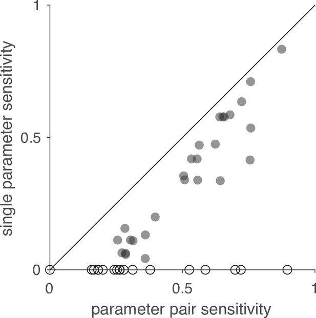
Comparison of sensitivity scores for changes of single and pairs of parameters.
Sensitivity scores obtained from changing single parameters and parameter pairs are correlated (Spearman’s rank correlation r = 0.88). The sensitivity scores for single parameters were obtained by quantifying how much the response field of LN4M changes when each of the 45 parameters selected for the analysis is changed individually (Figure 4F). Sensitivity scores for pairs were obtained by changing pairs of parameters (see Materials and methods). Open circles indicate parameters with zero sensitivity in the single parameter analysis and were excluded from the calculation of Spearman’s correlation.

Most responses fields are well fitted by ellipsoids, some are multi-peaked.
(A) Quantification of how well response fields (left column) are represented by ellipses. Ellipses (middle column) were fitted to binarized response fields (left column), obtained by thresholding each field at 50% of its maximum. The match between the binarized response field and the fitted ellipse was quantified using the Jaccard similarity, , which corresponds to the fraction of pixels that have the value 1 in the response field out of all pixels that are 1 in the field or the ellipse (intersection over union). Shown are two response fields that are well-fitted (top, = 0.69) or ill-fitted (bottom, = 0.38) by an ellipse. (B) Jaccard similarity for the responsive and selective response fields obtained by randomizing the model parameters. The distribution is heavily skewed towards high similarity values, indicating that most response fields are well fitted by ellipsoids. Vertical lines show the similarity values for the two examples in (A), 0.38 and 0.69. (C) Probability distribution of the asymmetry index for all response fields, given by the ratio of the ellipse’s major and minor axes. An asymmetry index of 1.0 means perfect symmetry, the higher the index, the more asymmetrical the response field. The inset shows three ellipses with asymmetry indices 1.25, 1.5, and 2.0. (D) Examples of multi-peaked response fields.

Response fields of all neurons in the network for examples from Figure 4E.
Shown are examples of response fields obtained by randomizing the model parameters with period tuning (A), duration tuning (B), duty cycle tuning (C), pause tuning (D), and a response field with multiple peaks (E). The colored lines show the 67% contour (33% contour in E) for LN4M in all panels. The phonotaxis response is coded in gray colors (see color bar).
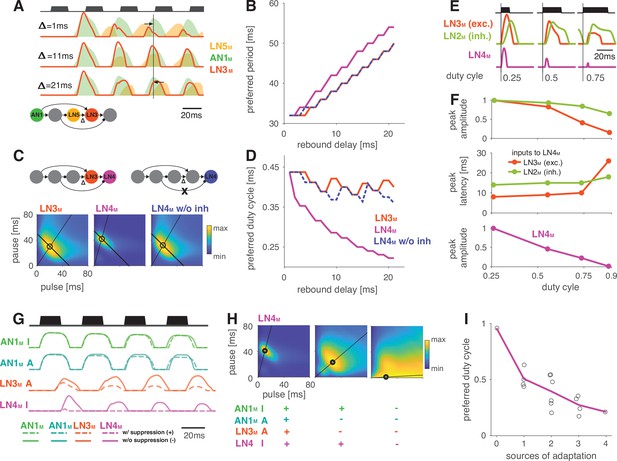
Input delays and response suppression control period and duty cycle preference.
(A) Inputs from LN5M and AN1M (orange and green shaded areas) to LN3M and output of LN3M (red line) for three input delays from LN5M to LN3M (‘rebound delay’ ). The rebound delay is defined as the delay added to the output of LN5M in the model. The effective delay between the AN1M and LN5M inputs to LN3M depends on the pulse pattern (black, top, pulse duration 20 ms, pause 18 ms). An intermediate delay of 11 ms produces the most overlap between the AN1M and LN5M inputs for that stimulus and hence the strongest responses in LN3M. Vertical black line marks an AN1M response peak, arrows point from the nearest LN5M response peak. (B) Preferred periods for LN3M (red), LN4M in an intact model (purple), and LN4M in a model without inhibition from LN2M to LN4M (blue) as a function of the rebound delay. The preferred period increases with rebound delay for all three cases. (C) Response fields for LN3M (left), LN4M in an intact network (middle), and for LN4M in a model without inhibition in LN4M from LN2M (right) (color coded, see color bar). The rebound delay was set to 21 ms, which increases the preferred period in both LN3M and LN4M to 50 ms (left, compare B). However, increasing the delay also decreases the preferred duty cycle in LN4M (middle). Removing the inhibition from LN2M in LN4M abolishes the change in duty cycle preference (right). Anti-diagonal lines mark the preferred period of 50 ms for each response field, and lines starting at the origin mark the preferred duty cycle. (D) Same as (B) but for the preferred duty cycle. With increasing delay, the preferred duty cycle for LN4M approaches 0.25 but is stable for LN3M and for LN4M without inhibition (Figure 5—figure supplement 2). (E) Inputs to LN4M (middle, green: inhibition from LN2M; red: excitation from LN3M) and output of LN4M (bottom, purple) for the intact network in (C) and for three different stimulus sequences with a pulse period of 54 ms and increasing duty cycles (top, black). Responses are shown for the second pulse in a train. Excitatory input from LN3M is weaker and overlaps more with the inhibition for high duty cycles (compare amplitude and latency of response peaks in LN3M), leading to a reduction in LN4M responses with increasing duty cycle. Y-scales are identical for all three panels and were omitted for clarity. (F) Dependence of peak amplitude (top) and peak latency (time from pulse onset to response peak, middle) of inputs to LN4M (red: excitation from LN3M; green: inhibition from LN2M) on pulse duty cycle for the intact network in (C). Weaker and later excitation suppresses LN4M responses for pulse trains with high duty cycles (bottom, purple). (G) Four sources of suppression in the network: the inhibitory lobe in the filter of AN1M (green), adaptation in AN1M (cyan) and LN3M (red), and inhibition in LN4M from LN2M (purple). Shown are responses to a pulse pattern (top black, 20 ms pulse duration and 20 ms pause) when the source of suppression is present (dashed lines) or absent (solid lines). Removing suppression produces stronger or more sustained responses. ‘A’ and ‘I’ refer to adaptation and inhibition, respectively. (H) Response fields (color coded, see color bar) for the network output (LN4M) after removing different sources of suppression. The presence or absence of different sources of suppression is marked with a ‘+’ and a ‘–’, respectively. Removing suppression in the network increases the preferred duty cycle. Lines mark the preferred pulse duty cycle, and black dots indicate the preferred pulse duration and pause. (I) Preferred duty cycle in LN4M as a function of the number of sources of adaption present in the model. Black dots show the preferred duty cycle of individual model variants, the purple line shows the average over models for a given number of adaptation sources. Adaptation decreases the preferred duty cycle (Pearson’s r = 0.78, p=3 × 10⁻⁴). See Figure 2—figure supplement 1 for details. The pulse trains for all simulations in this figure had a duration of 600 ms and were interleaved by chirp pauses of 200 ms to ensure that trains contained enough pulses even for long pulse durations and pauses. Rebound delay set to 21 ms in (C) and (E–I) to make changes in the duty cycle preference more apparent.
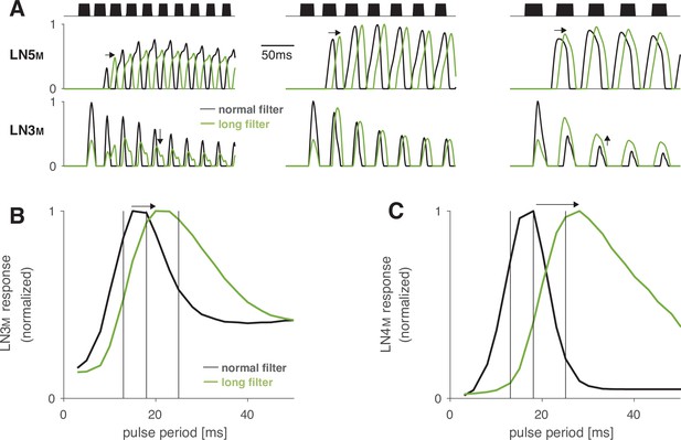
Increasing the duration of the postsynaptic filter in LN5M delays rebound responses and increases the preferred pulse period in LN3M.
(A) Rebound responses of LN5M (top) and responses of the coincidence detector LN3M (bottom) for models with a normal (black) and a long (green) postsynaptic filter in LN5M (Figure 2—figure supplement 2). The three stimuli (black) have pulse periods of 12, 16, and 24 ms (from left to right) and duty cycles of 0.5. Increasing the filter duration delays rebound responses in LN5M (middle row, arrows) and therefore shifts the pulse period at which LN3M is most strongly driven towards higher values (bottom row, arrows). (B, C) Period tuning of LN3M (B) and of the network output LN4M (C) for LN5M with a normal (5 ms, black) and a long (31 ms, green) postsynaptic filter. The differentiating postsynaptic filter (Figure 2—figure supplement 2) mediates adaptation and saturation of the inputs to the rebound filter in LN5M (Figure 2—figure supplement 1). Increasing the filter duration increases the preferred pulse period in LN3M (B), and this effect is further amplified in LN4M (C). Vertical black lines indicate the periods for the stimuli shown in (A). Response traces (A) and tuning curves (B, C) were normalized to peak at 1.0.
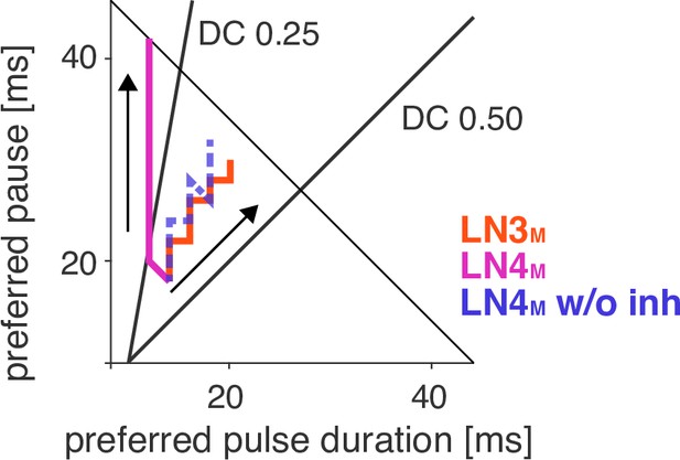
Preferred pulse and pause parameters for LN3M (red), LN4M (purple), and LN4M without inhibition from LN2M over the range of rebound delays tested in Figure 5B and D (1–21 ms).
Arrows point in the direction of increasing delays. The anti-diagonal line marks the pulse period of 50 ms, and the diagonal lines mark the pulse duty cycles (DCs) of 0.25 and 0.5. With increasing delay, the preferred duty cycle for LN4M approaches 0.25 but is stable at around 0.45 for LN3M and LN4M without inhibition (compare Figure 5D).
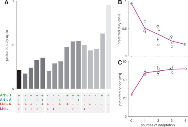
Adaptation decreases the preferred duty cycle and has weak effects on the preferred period.
(A) Preferred duty cycles for models with different sources of suppression present (+) or absent (–) (Figure 5G). ‘I’ and ‘A’ denote inhibition and adaption, respectively. (B, C) Preferred duty cycle (B) and period (C) as a function of the number of sources of suppression present in the model. The preferred duty cycle decreases with suppression, while the preferred period remains relatively constant. The preferred period for a model without adaptation (zero sources of adaptation) is reduced because this model was tuned for duty cycle, with very broad selectivity for period (Figure 5H, rightmost panel).
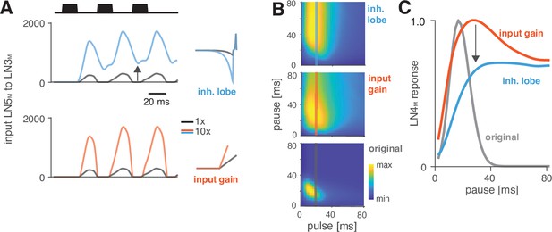
Changes in LN5M rebound dynamics induce a switch in response type.
(A) Increasing the amplitude of the inhibitory lobe of the filter in LN5M that generates the rebound (middle, blue, ‘inhibitory lobe’) increases the rebound’s amplitude and duration. By contrast, the gain of the input from LN5M to LN3M (bottom, red, ‘input gain’) scales the input from the LN5M rebound without prolonging it. Pictograms on the right show the parameters for the original model (black) and for a model with a 10-fold increase in the respective parameter value (blue and red). Traces show the rebound inputs from LN5M to LN3M for the pulse pattern shown on top (black traces, 20 ms pulse duration and 20 ms pause). (B) Response fields of LN4M for the original model (bottom), and for models with increased inhibitory lobe (top) or input gain (middle). Response magnitudes are color coded (see color bar, scaled to span the range of response magnitudes). Amplifying and prolonging the rebound by increasing the inhibitory lobe (top) produces pause tuning, while only amplifying the rebound via the input gain retains period tuning (bottom). Vertical lines correspond to the stimuli for which pause tuning curves are shown in (C). (C) Pause tuning curves for LN4M at a pulse duration of 20 ms (see lines in B) reveal differential effects of the parameters on pause tuning. Amplifying and prolonging the rebound by increasing the inhibitory filter lobe (blue) produces high tolerance for pause duration, in this case high-pass tuning, which is required to obtain duration tuning. By contrast, only amplifying the rebound via the input gain (red) retains the preference for intermediate pauses characteristic for period tuning. The pulse trains had a duration of 600 ms and were interleaved by chirp pauses of 200 ms for all simulations to ensure that the stimuli in the response fields contained enough pulses even for long pulse durations and pauses.

Sustained rebound responses in LN5M induce stronger adaptation in LN3M for pulse patterns with short pauses.
Traces of LN5M→LN3M inputs (middle) and LN3M responses (bottom) for models with 10-fold increased input gain (red) or inhibitory lobe (blue). The sustained rebound response for pulse trains with short pauses in models with an increased inhibitory lobe (blue, middle) leads to stronger adaptation in LN3M (blue, bottom). This reduces responses specifically for pulse patterns with short pauses (bottom, first two panels) and causes the switch from bandpass to high-pass tuning for pulse pause (Figure 6). Arrows indicate changes of opposing sign in the input to LN3M (middle) and the responses of LN3M (bottom). Stimuli (top, black) have pulse durations of 10 ms and pauses of 5, 15, and 35 ms.
Tables
Model parameters.
See Figure 2—figure supplement 1 and Figure 2—figure supplement 2 for an illustration and methods for a definition of all parameters. * marks parameters that were fixed during training (9/55). † marks parameters that were fixed during parameter and sensitivity analyses (10/55, Figures 4—6).
| Cell | Component | Parameters |
|---|---|---|
| AN1M | Filter excitatory lobe | (Gaussian) width =0.0005, duration = 9.88 ms, input delay = 7.41 ms |
| Filter inhibitory lobe | (Gaussian) width =2.32, gain =0.06, duration N = 184 ms | |
| Nonlinearity | (Sigmoidal) slope = 1.5, shift = 1.5, gain = 5, baseline = −0.5 | |
| Adaptation | (Divisive normalization) timescale =3760 ms, strength w = 2.82, offset x0 = 1*† | |
| Output gain | Gain=12.8† | |
| LN2M | Input from AN1M | Delay = 0 ms, gain = 0.19 |
| Filter excitatory lobe | (Gaussian) width =1.07, duration N = 14.2 ms, gain = 0.272 | |
| Filter inhibitory lobe | (Exponential) decay =5.98 ms, duration N = 1000 ms*† | |
| Output nonlinearity | (Rectifying) threshold = 0*†, gain = 1.33 | |
| LN5M | Input from LN2M | Delay = 8.39 ms, gain = −0.005 |
| Postsynaptic filter | (Differentiated Gaussian) duration N = 5.0 ms, width =3.5*†, gain of the excitatory lobe = 1.15 | |
| Postsynaptic nonlinearity | (Rectifying) threshold = 0*†, gain = 1*† | |
| Rebound filter exc. lobe | (Exponential) decay =3.54 ms, duration N = 20.7 ms, gain = 915 | |
| Rebound filter inh. lobe | (Exponential) decay =30.3 ms, duration N = 500 ms*†, gain = 1718 | |
| Output nonlinearity | (Rectifying) threshold = 0*†, gain = 3.82 | |
| LN3M | Input from AN1M | Delay = 7.33 ms, gain = 32.1 |
| Input from LN5M | Delay = 3.16 ms, gain = 3.78 | |
| Postsyn. nonlinearity | (Rectifying) threshold = 0.26, gain = 0.014 | |
| Adaptation | (Divisive normalization) timescale =39.4 ms, strength w = 0.283, offset x0 = 1*† | |
| Output nonlinearity | (Rectifying) threshold = 2.33, gain = 7.68 | |
| LN4M | Input from LN2M | Delay = 17 ms, gain = –1205 |
| Input from LN3M | Delay = 4.87 ms, gain = 401 | |
| Output nonlinearity | (Rectifying) threshold = 738, gain = 0.0052 |


