Figures and data in Binocular rivalry reveals an out-of-equilibrium neural dynamics suited for decision-making | eLife

15 figures

Figures

Figure 1

Download asset Open asset

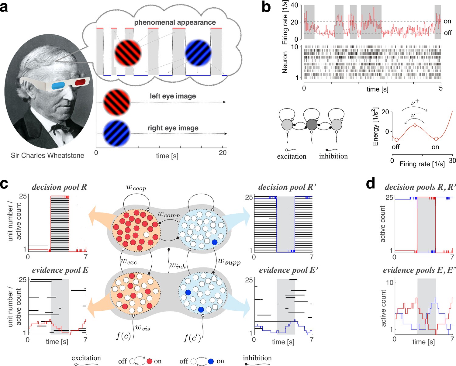
Proposed mechanism of binocular rivalry.

(a) When the left and right eyes see incompatible images in the visual field, phenomenal appearance reverses at irregular intervals, sometimes being dominated by one image and sometimes by the other (gray and white regions). Sir Charles Wheatstone studied this multistable percept with a mirror stereoscope (not as shown!). (b) Spiking neural network implementation of a ‘local attractor.’ An assembly of 150 neurons (schematic, dark gray circle) interacts competitively with multiple other assemblies (light gray circles). Population activity of the assembly explores an effective energy landscape (right) with two distinct steady states (circles), separated by a ridge (diamond). Driven by noise, activity transitions occasionally between ‘on’ and ‘off’ states (bottom), with transition rates $ν^{\pm}$ depending sensitively on external input to the assembly (not shown). Here, $ν^{+} = ν^{-} \approx 1 H z$ . Spike raster shows 10 representative neurons. (c) Nested attractor dynamics (central schematic) that quantitatively reproduces the dynamics of binocular rivalry (left and right columns). Independently bistable variables (‘local attractors,’ small circles) respond probabilistically to input, transitioning stochastically between on- and off-states (red/blue and white, respectively). The entire system comprises four pools, with 25 variables each, linked by excitatory and inhibitory projections. Phenomenal appearance is decided by competition between decision pools $R$ and $R^{'}$ forming ‘non-local attractors’ (cross-inhibition $w_{c o m p}$ and self-excitation $w_{c o o p}$ ). Visual input $c$ and $c^{'}$ accumulates, respectively, in evidence pools $E$ and $E^{'}$ and propagates to decision pools (feedforward selective excitation $w_{e x c}$ and indiscriminate inhibition $w_{i n h}$ ). Decision pools suppress associated evidence pools (feedback selective suppression $w_{s u p p}$ ). The time course of the number of active variables (active count) is shown for decision pools (top left and right) and evidence pools (bottom left and right), representing the left eye (red traces) and the right eye image (blue traces). The state of individual variables (black horizontal traces in left and middle columns) and of perceptual dominance (gray and white regions) is also shown. In decision pools, almost all variables become active (black trace) or inactive (no trace) simultaneously. In evidence pools, only a small fraction of variables is active at any given time. (d) Fractional activity dynamics of decision pools $R$ and $R^{'}$ (top, red and blue traces) and evidence pools $E$ and $E^{'}$ (bottom, red and blue traces). Reversals of phenomenal appearance are also indicated (gray and white regions).

Figure 2

Download asset Open asset

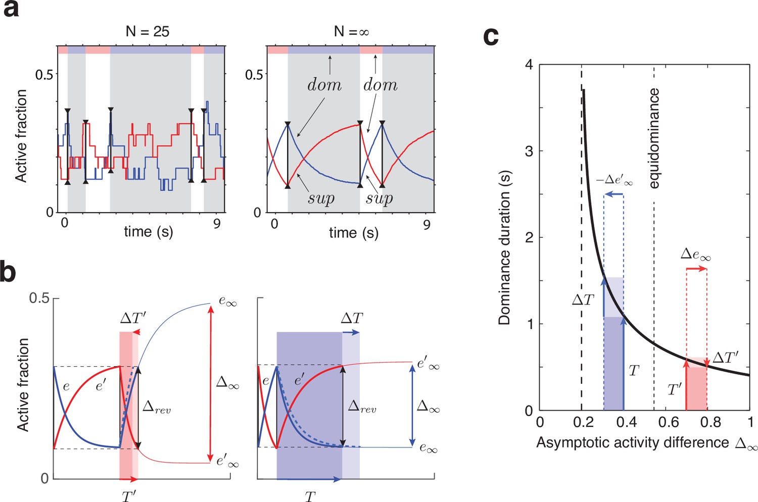
Joint dynamics of evidence habituation and recovery.

Exponential development of evidence activities is governed by input-dependent asymptotic values and characteristic times. (a) Fractional activities $e$ (blue traces) and $e^{'}$ (red traces) of evidence pools $E$ and $E$ , respectively, over several dominance periods for unequal stimulus contrast ( $c = \frac{7}{8}, c^{'} = \frac{1}{8}$ ). Stochastic reversals of finite system ( $N = 25$ units per pool, left) and deterministic reversals of infinite system ( $N$ , right). Perceptual dominance (decision activity) is indicated along the upper margin (red or blue stripe). Dominance evidence habituates (dom), and non-dominant evidence recovers (sup), until evidence contradicts perception sufficiently (black vertical lines) to trigger a reversal (gray and white regions). (b) Development of stronger-input evidence $e$ (blue) and weaker-input evidence $e^{'}$ (red) over two successive dominance periods ( $c = \frac{15}{16}, c^{'} = \frac{1}{16}$ ). Activities recover, or habituate, exponentially until reversal threshold $Δ_{r e v}$ is reached. Thin curves extrapolate to the respective asymptotic values, $e_{\infty}$ and ${e^{'}}_{\infty}$ . Dominance durations depend on distance $Δ_{\infty}$ and on characteristic times $τ_{e}$ and $τ_{e^{'}}$ . Left: incrementing non-dominant evidence $e$ (dashed curve) raises upper asymptotic value $e_{\infty}$ and shortens dominance $T^{'}$ by $Δ T^{'}$ . Right: incrementing dominant evidence $e$ (dashed curve) raises lower asymptotic value $e_{\infty}$ and shortens dominance $T$ by $Δ T$ . (c) Increasing asymptotic activity difference $Δ_{\infty}$ accelerates the development of differential activity and curtails dominance periods $T$ , $T^{'}$ (and vice versa). As the dependence is hyperbolic, any change to $Δ_{\infty}$ disproportionately affects longer dominance periods. If $T §gt; T^{'}$ , then $Δ T §gt; Δ T^{'}$ (and vice versa).

Figure 3

Download asset Open asset

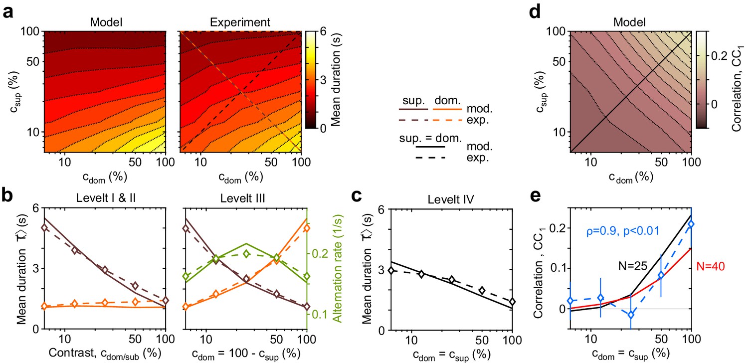
Dependence of mean dominance duration on dominant and suppressed image contrast (‘Levelt’s propositions’).

(a) Mean dominance duration $⟨ T ⟩$ (color scale), as a function of dominant contrast $c_{d o m}$ and suppressed contrast $c_{s u p}$ , in model (left) and experiment (right). (b) Model prediction (solid traces) and experimental observation (dashed traces and symbols) compared. Levelt I and II: weak increase of $⟨ T ⟩$ with $c_{d o m}$ when $c_{s u p} = 1$ (red traces and symbols), and strong decrease with $c_{s u p}$ when $c_{d o m} = 1$ (brown traces and symbols). Levelt III: symmetric increase of $⟨ T ⟩$ with $c_{d o m}$ (orange traces and symbols) and decrease with $c_{s u p}$ (brown traces and symbols), when $c_{d o m} + c_{d o m} = 1$ . Alternation rate (green traces and symbols) peaks at equidominance and decreases symmetrically to either side. (c) Levelt IV: decrease of $⟨ T ⟩$ with image contrast, when $c_{s u p} = c_{d o m}$ . (d) Predicted dependence of sequential correlation $c c_{1}$ (color scale) on $c_{d o m}$ and $c_{s u p}$ . (e) Model prediction (black trace, $N = 25$ ) and experimental observation (blue trace and symbols, mean ± SEM, Spearman’s rank correlation ρ), when $c_{s u p} = c_{d o m}$ . Also shown is a second model prediction (red trace, $N = 40$ ).

Figure 4

Download asset Open asset

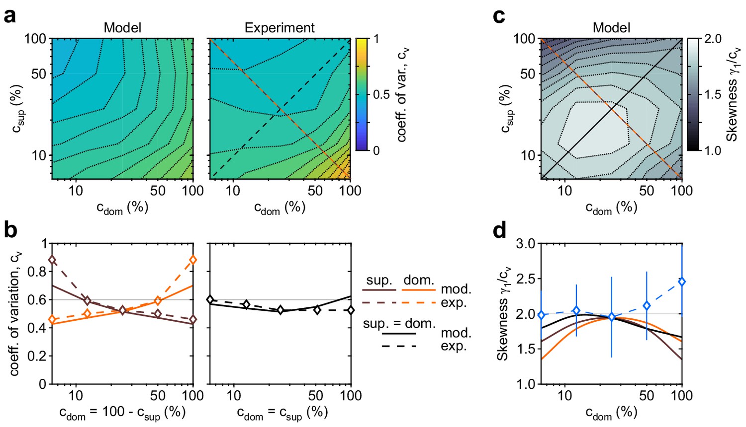
Shape of dominance distribution depends only weakly on image contrast (‘scaling property’).

Distribution shape is parametrized by coefficient of variation c_v and relative skewness $γ_{1} / c_{V}$ . (a) Coefficient of variation c_v (color scale), as a function of dominant contrast $c_{d o m}$ and suppressed contrast $c_{s u p}$ , in model (left) and experiment (right). (b) Model prediction (solid traces) and experimental observation (dashed traces and symbols) compared. Left: increase of c_v with $c_{d o m}$ (red traces and symbols), and symmetric decrease with $c_{s u p}$ (brown traces and symbols), when $c_{s u p} = 1$ . Right: weak dependence when $c_{d o m} = c_{s u p}$ (black traces and symbols). (c) Predicted dependence of relative skewness $γ_{1} / c_{V}$ (gray scale) on $c_{d o m}$ and $c_{s u p}$ . (d) Model prediction (solid traces), when $c_{d o m} = c_{s u p}$ (black) and $c_{d o m} = 1 - c_{s u p}$ (orange and brown) and experimental observation when $c_{d o m} = c_{s u p}$ (blue dashed trace and symbols, mean ± SEM).

Figure 5

Download asset Open asset

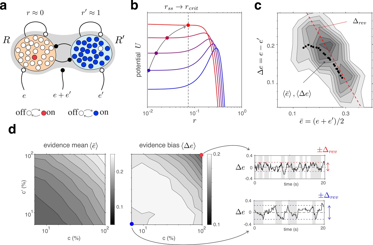
Competitive dynamics of decision pools ensures Levelt IV.

(a) The joint stable state of decision pools (here $r^{'} ≃ 1$ and $r ≃ 0$ ) can be destabilized by sufficiently contradictory evidence, $e §gt; e^{'}$ . (b) Effective potential $U (e, e^{'}, r, r^{'})$ (colored curves) and steady states $r_{\infty}$ (colored dots) for different levels of contradictory input, $Δ e = e - e^{'}$ . Increasing $Δ e$ destabilizes the steady state and shifts $r_{\infty}$ rightward (curved arrow). The critical value $r_{c r i t}$ (dotted vertical line), at which the steady state turns unstable, is reached when $Δ e$ reaches the reversal threshold $Δ_{r e v}$ . At this point, a reversal ensues with $r \to 1$ and $r^{'} \to 0$ . (c) The reversal threshold $Δ_{r e v}$ diminishes with combined evidence $e + e^{'}$ . In the deterministic limit, $Δ_{r e v}$ decreases linearly with $\bar{e} = (e + e^{'}) / 2$ (dashed red line). In the stochastic system, the average evidence bias $⟨ Δ e ⟩$ at the time of reversals decreases similarly with the average evidence mean $⟨ \bar{e} ⟩$ (black dots). Actual values of $Δ e$ at the time of reversals are distributed around these average values (gray shading). (d) Average evidence mean $⟨ \bar{e} ⟩$ (left) and average evidence bias $⟨ Δ e ⟩$ (middle) at the time of reversals as a function of image contrast $c$ and $c^{'}$ . Decrease of average evidence bias $⟨ Δ e ⟩$ with contrast shortens dominance durations (Levelt IV). At low contrast (blue dot), higher reversal thresholds $Δ_{r e v}$ result in less frequent reversals (bottom right, gray and white regions) whereas, at high contrast (red dot), lower reversal thresholds lead to more frequent reversals (top right).

Figure 6

Download asset Open asset

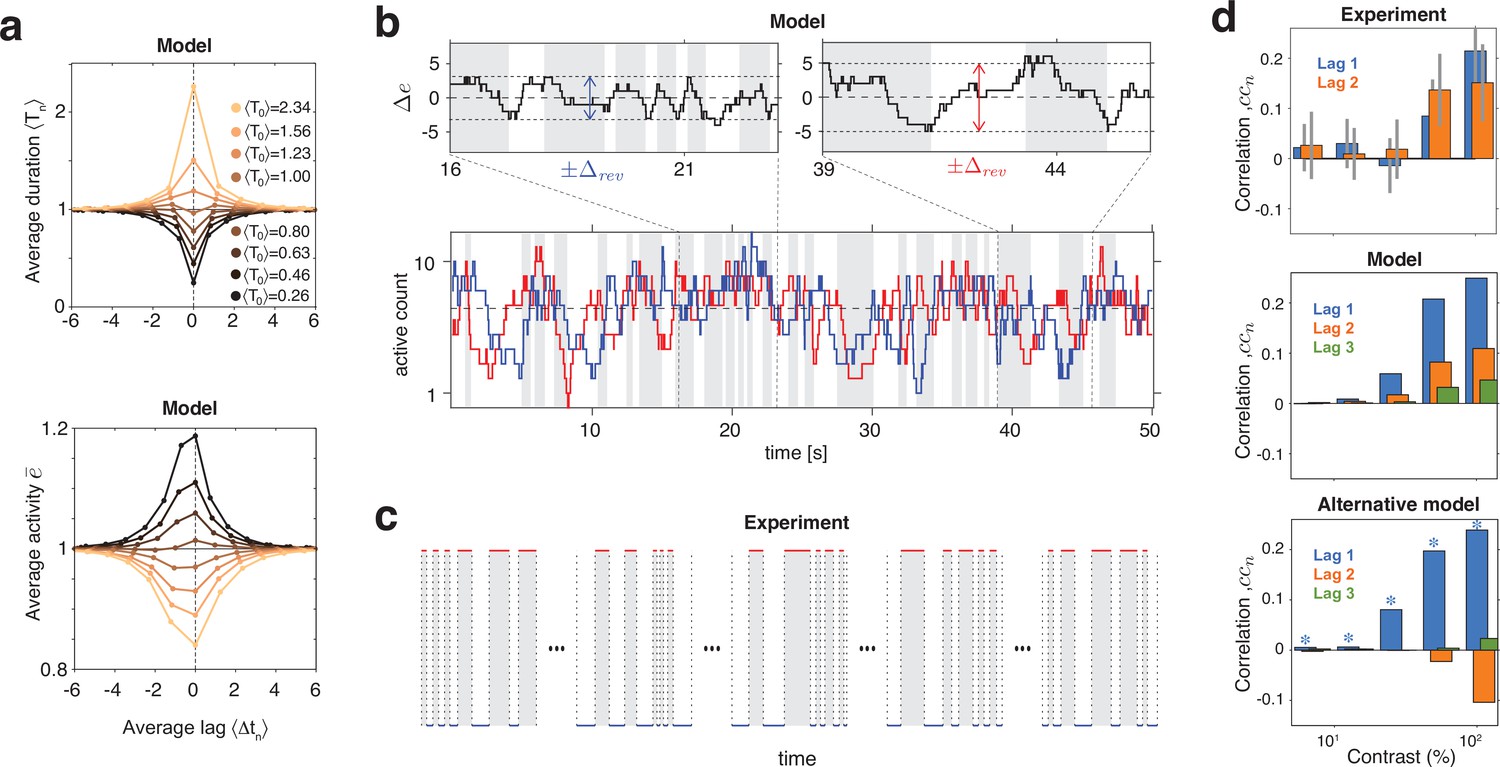
Serial dependency predicted by model and confirmed by experimental observations.

(a) Conditional expectation of dominance duration $⟨ T_{\pm n} ⟩$ (top) and of average mean evidence activity, $⟨ {\bar{e}}_{\pm n} ⟩$ (bottom), in model simulations with maximal stimulus contrast ( $c = c^{'} = 1$ ). Dominance periods T₀ were grouped into octiles, from longest (yellow) to shortest (black). For each octile, the average duration $⟨ T_{\pm n} ⟩$ of preceding and following dominance periods, as well as the average mean evidence activity $⟨ {\bar{e}}_{\pm n} ⟩$ at the end of each period, is shown. All times in multiples of the overall average duration, $⟨ T ⟩$ , and activities in multiples of the overall average activity $⟨ \bar{e} ⟩$ . (b) Example reversal sequence from model. Bottom: stochastic development of evidence activities $e$ and $e^{'}$ (red and blue traces), with large, joint fluctuations raising or lowering mean activity $\bar{e} = (e + e^{'}) / 2$ above or below long-term average (dashed line). Top left: episode with $\bar{e}$ above average, lower $Δ_{r e v}$ , and shorter dominance periods. Top right: episode with $\bar{e}$ below average, higher $Δ_{r e v}$ , and longer dominance durations. (c) Examples of reversal sequences from human observers ( $c = c^{'} = 1$ and $c = c^{'} = 1 / 2$ ). (d) Positive lagged correlations predicted by model (mean, middle) and confirmed by experimental observations (mean ± std, top). Alternative model (Laing and Chow, 2002) with adaptation and noise (mean, bottom), fitted to reproduce the values of $⟨ T ⟩$ , c_v, $γ_{1}$ , and $c c_{1}$ predicted by the present model (blue stars).

Appendix 1—figure 1

Download asset Open asset

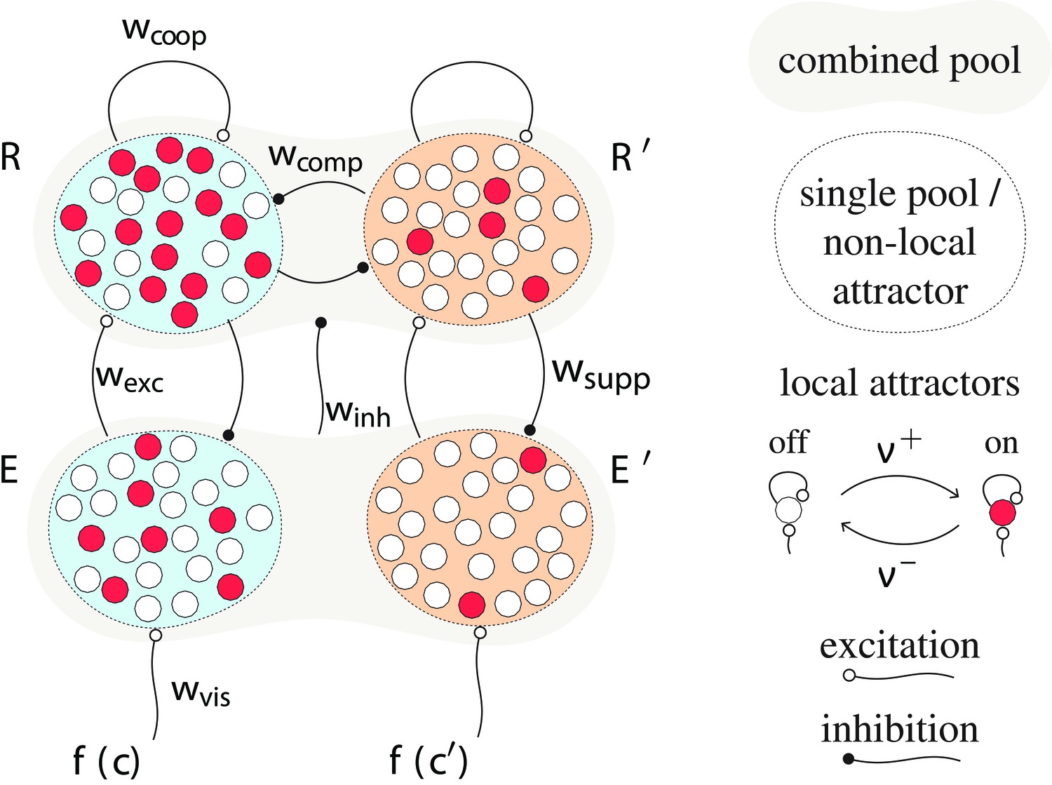
Proposed mechanism of binocular rivalry dynamics (schematic).

Bistable variables are represented by white (inactive) or red (active) circles. Four pools, each with $N = 25$ variables, are shown: two evidence pools $E$ and $E^{'}$ , with active counts $n_{e} (t)$ and $n_{e^{'}} (t)$ , and two decision pools, $R$ and $R^{'}$ , with active counts $n_{r} (t)$ and $n_{r^{'}} (t)$ . Excitatory and inhibitory synaptic couplings include selective feedforward excitation $w_{e x c}$ , indiscriminate feedforward inhibition $w_{i n h}$ , recurrent excitation $w_{c o o p}$ , and mutual inhibition $w_{c o m p}$ of decision pools, as well as selective feedback suppression $w_{s u p p}$ of evidence pools. Visual input to evidence pools $f (c)$ and $f (c^{'})$ is a function of image contrast $c$ and $c^{'}$ .

Appendix 1—figure 2

Download asset Open asset

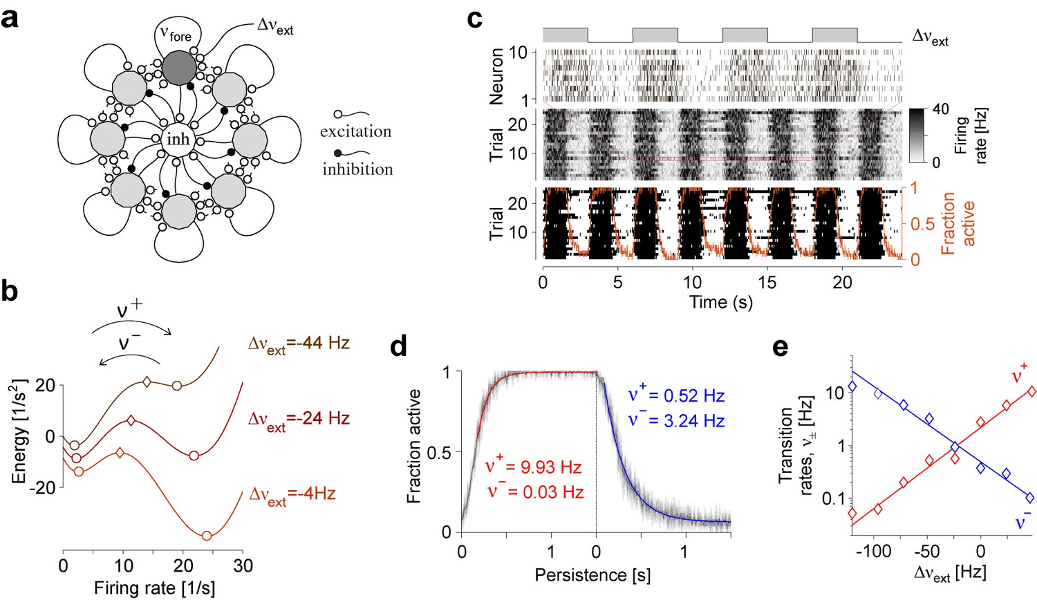
Metastable dynamics of spiking neural network.

(a) Eight assemblies of excitatory neurons (schematic, light and dark gray disks) and one pool of inhibitory neurons (white disc) interact competitively with recurrent random connectivity. We focus on one ‘foreground’ assembly (dark gray), with firing rate $ν_{f o r e}$ and selective external input $Δ ν_{e x t}$ . (b) ‘Foreground’ activity explores an effective energy landscape with two distinct steady states (circles), separated by ridge points (diamonds). As this landscape changes with external input $Δ ν_{e x t}$ , transition rates $ν^{\pm}$ between ‘on’ and ‘off’ states also change with external input. (c) Simulation to establish transition rates $ν^{\pm}$ of foreground assembly. External input $Δ ν_{e x t}$ is stepped periodically between $- 44 H z$ and $- 4 H z$ . Spiking activity of 10 representative excitatory neurons in a single trial, population activity over 25 trials, thresholded population activity over 25 trials, and activation probability (fraction of ‘on’ states). (d) Relaxation dynamics in response to step change of $Δ ν_{e x t}$ , with ‘on’ transitions (left) and ‘off’ transitions (right). (e) Average state transition rates $ν^{\pm}$ vary anti-symmetrically and exponentially with external input: $ν^{+} ≃ 2.2 H z \exp (+ 0.8 5 s Δ ν_{e x t})$ and $ν^{-} ≃ 0.5 H z \exp (- 0.79 s Δ ν_{e x t})$ (red and blue lines).

Appendix 1—figure 3

Download asset Open asset

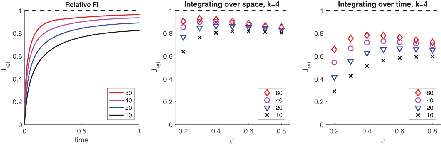
Information retained by stochastic pool activity from normally distributed inputs.

Inputs $s \in N (μ, σ)$ provide Fisher information $J_{s} = \frac{1}{σ^{2}}$ about mean $μ$ . Stochastic activity $n (t)$ of a birth-death process ( $N \in {10, 20, 40, 80}$ and $w = 2.5$ ) driven by such inputs accumulates Fisher information $J_{n} (t)$ about mean $μ$ . (a) Accumulation over input interval $t = [0, 1]$ of fractional information $J_{r e l} (t) = J_{n} (t) σ^{2}$ by an initially inactive pool of size $N$ . (b) Information about μ retained by summed activity $\hat{n} = n_{1} + \dots + n_{4}$ of four independent pools (all initially inactive and of size $N$ ) receiving concurrently four independent inputs ( $s \in N (μ, σ)$ ) over an interval $t = [0, 1]$ . Retained fraction $J_{r e l} = J_{\hat{n}} (1) σ^{2} / 4$ depends on pool size $N$ and input variance $σ^{2}$ . (c) Information about $μ$ retained by activity $n$ of one pool (initially inactive and of size $N$ ) receiving successively four independent inputs ( $s \in N (μ, σ)$ ) over an interval $t = [0, 4]$ . Retained fraction $J_{r e l} = J_{n} (4) σ^{2} / 4$ depends on pool size $N$ and input variance $σ^{2}$ .

Appendix 1—figure 4

Download asset Open asset

Decision response to fixed input $I$ , $I^{'}$ , for random initial conditions of $e$ , $e^{'}$ , $r$ , $r^{'}$ .

(a) Expected differential steady-state activation $⟨ | r - r^{'} | ⟩$ of decision level. Steady-state activity $r + r^{'} ≃ 1$ implies a categorical decision with activity $≃ 1$ of one pool and activity of another. (b) Probability that decision correctly reflects input bias ( $r §gt; r^{'}$ if $I §gt; I^{'}$ ), and vice versa.

Appendix 1—figure 5

Download asset Open asset

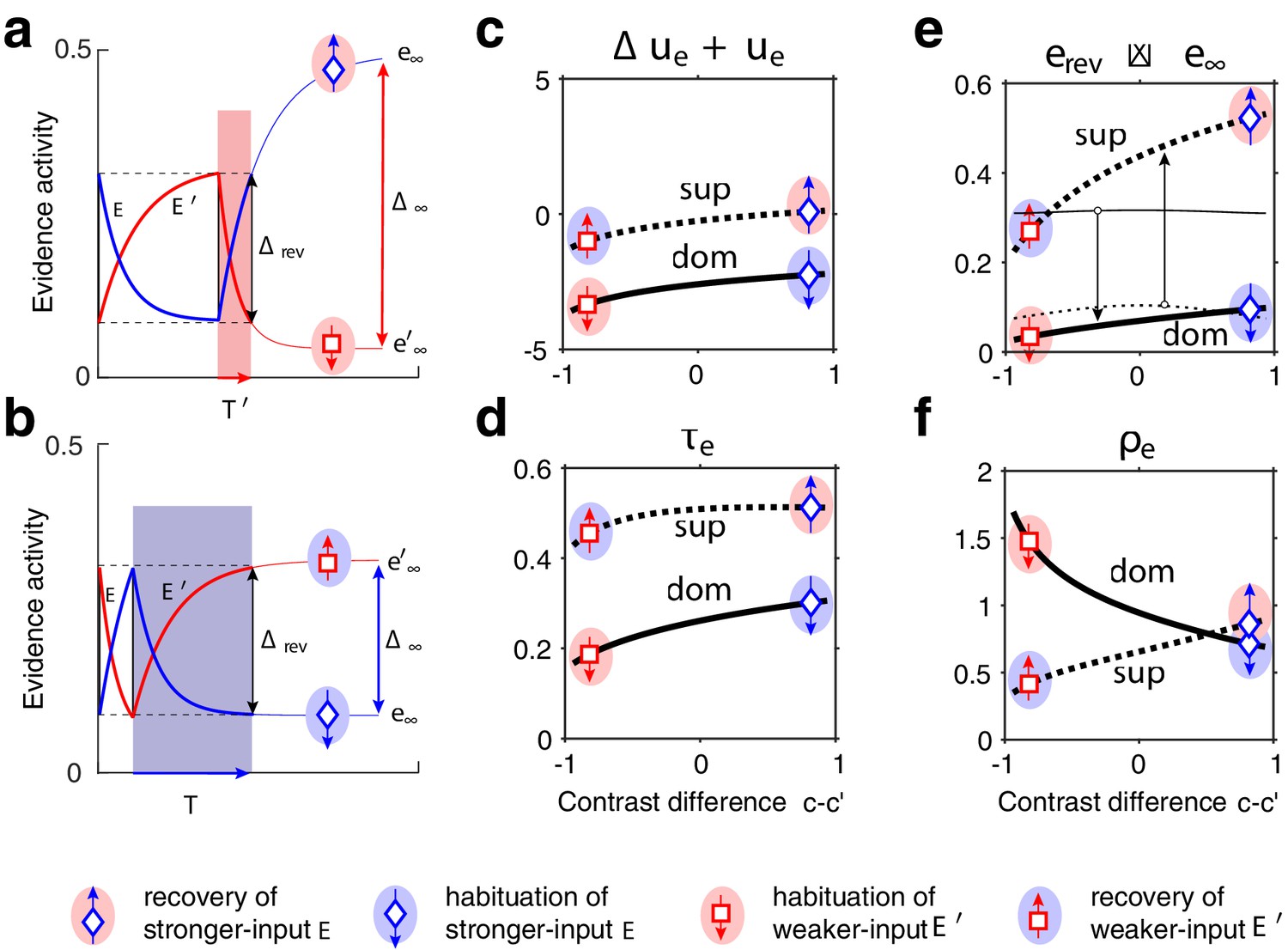
Exponential habituation and recovery of evidence activities.

Dominance durations depend on distance between asymptotic values and on characteristic times. (a, b) Development of evidence $e$ (blue) and $e^{'}$ (red), over two successive dominance periods. Input $c = 15 / 16$ is stronger, input $c^{'} = 1 / 16$ weaker. Activities recover, or habituate, exponentially until reversal threshold $Δ_{r e v}$ is reached. Thin curves extrapolate to the respective asymptotic values, $e_{\infty}$ and ${e^{'}}_{\infty}$ . (a) Evidence $e^{'}$ (with weaker input $c^{'}$ ) is dominant. Incrementing input $c$ to non-dominant evidence $e$ shortens dominance $T^{'}$ . (b) Evidence $e$ (with stronger input $c$ ) is dominant. Incrementing input $c$ to $e$ extends dominance $T$ . (c–f) Contrast dependence of relaxation dynamics, as a function of differential contrast $c - c^{'}$ , for $c + c^{'} = 1$ . Values when evidence $e$ is dominant (dom, thick solid curves), and when it is non-dominant (sup, thick dotted curves). Values for $e^{'}$ are mirror symmetric (about vertical midline $c - c^{'} = 0$ ). (c) Effective potential $Δ u_{e} + u_{e}$ . (d) Characteristic time $τ_{e}$ . (e) Relaxation range $e_{r e v} \to e_{\infty}$ (bottom left, thin curves $e_{r e v}$ , thick curves $e_{\infty}$ ). (f) Effective rate $ρ_{e}$ of development. Symbols and arrows correspond to subfigures (a, b) and represent recovery (up arrow) or habituation (down arrow) of stronger-input evidence (blue) or weaker-input evidence (red). Underlying color patches indicate dominance of stronger-input evidence (blue patches) or of weaker-input evidence (red patches). Dominance durations depend more sensitively on the slower development, with smaller $ρ$ , which generally is the recovery of non-dominant evidence (up arrows).

Appendix 1—figure 6

Download asset Open asset

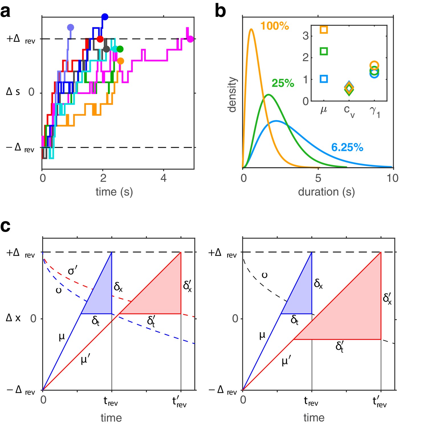
Birth-death dynamics of evidence pools ensures gamma-like distribution and ‘scaling property’ (invariance of distribution shape).

(a) Representative examples for the time development of evidence bias $Δ e = e - e^{'}$ between reversals (i.e., between $- Δ_{r e v}$ and approximately $+ Δ_{r e v}$ ). (b) Dominance distributions for $c = c^{'} = 1 / 16$ (blue), $c = c^{'} = 1 / 4$ (green), and $c = c^{'} = 1$ (yellow). Distribution mean $μ$ changes approximately threefold, but coefficient of variation $c_{V}$ and skewness $γ_{1}$ are nearly invariant (inset), largely preserving distribution shape. (c) Development of expectation $⟨ Δ x ⟩$ between reversals (schematic). Left: a Poisson variable process, such as the difference $Δ x$ between two birth-death processes. Mean $⟨ Δ x ⟩$ grows linearly with $t$ (lines, with slopes $μ$ , $μ^{'}$ ) and variance $⟨ (Δ x - ⟨ Δ x ⟩)^{2} ⟩$ grows linearly with $\sqrt{t}$ (dashed curves, with scaling factors $σ$ , $σ^{'}$ ). Constants $μ$ and $σ$ change with stimulus contrast (blue and red). Proportionality $μ \propto σ^{2}$ ensures constant dispersion of $Δ x$ at threshold ( $δ_{x} = δ_{x}^{'}$ ), and, consequently, a dispersion of threshold-crossing times that grows linearly with mean threshold-crossing time ( $δ_{t} / t_{r e v} = δ_{t}^{'} / t_{r e v}^{'} = c o n s t$ ), preserving distribution shape. Right: a process with constant variance, $σ = σ^{'}$ . Dispersion of $Δ x$ at threshold increases with threshold-crossing time ( $δ_{x}^{'} §gt; δ_{x}$ ) and dispersion of threshold-crossing times grows supra-linearly with mean threshold-crossing time ( $δ_{t} / t_{rev}$ < $δ_{t} / t_{r e v} §lt; δ_{t}^{'} / t_{r e v}^{'}$ ), broadening distribution shape.

Appendix 1—figure 7

Download asset Open asset

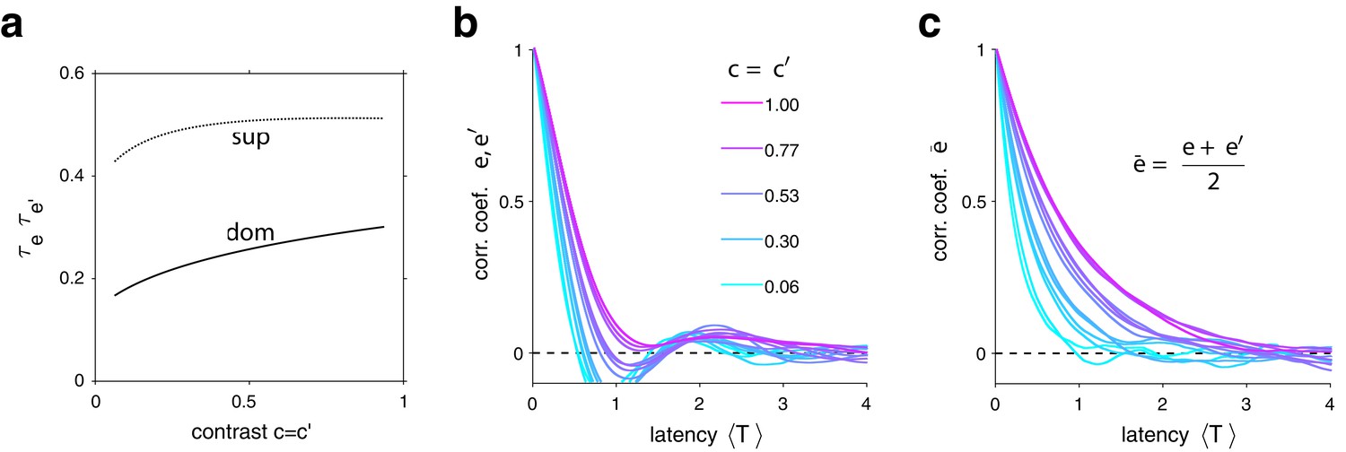
Characteristic times of evidence activity.

(a) Characteristic times $τ_{e}$ , $τ_{e^{'}}$ for different image contrast $c$ = $c^{'}$ , when evidence pool is dominant (dom) and non-dominant (sup). (b) Autocorrelation of evidence activity $e$ , $e^{'}$ as a function of image contrast (color) and latency, expressed in multiples of average dominance duration $⟨ T ⟩$ . (c) Autocorrelation of joint evidence activity $\bar{e} = (e + e^{'}) / 2$ as a function of image contrast (color) and latency. Note that autocorrelation time lengthens substantially for high image contrast.

Appendix 1—figure 8

Download asset Open asset

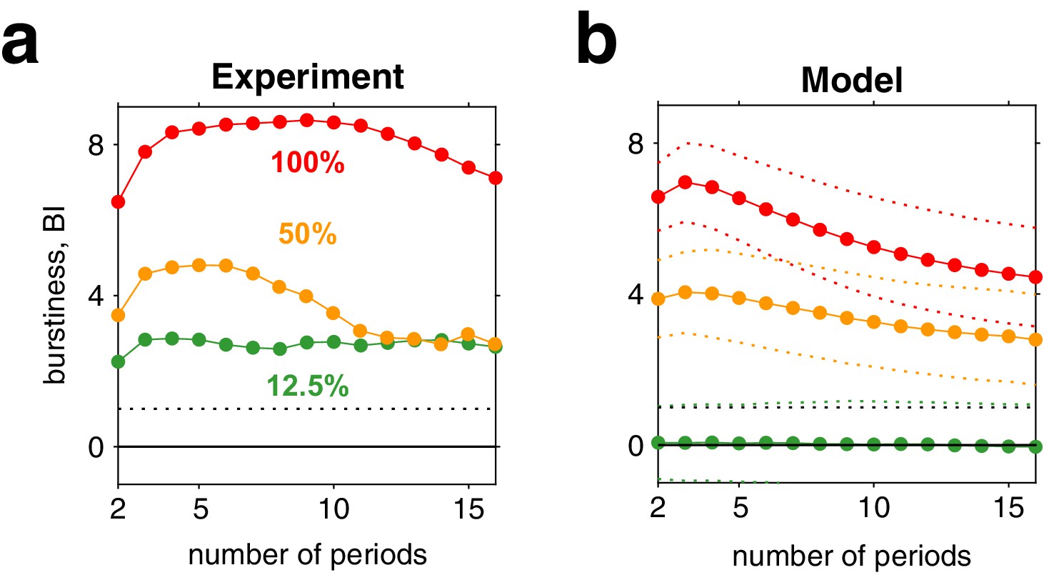
Burstiness of reversal sequences predicted by model and confirmed by experimental observations.

(a) Burstiness index (BI) (mean) for $n$ successive dominance periods in experimentally observed reversal sequences, for contrasts 12.5% (green), 50% (yellow), and 100% (red). (b) BI for reversal sequences generated by model (mean ± std).

Appendix 1—figure 9

Download asset Open asset

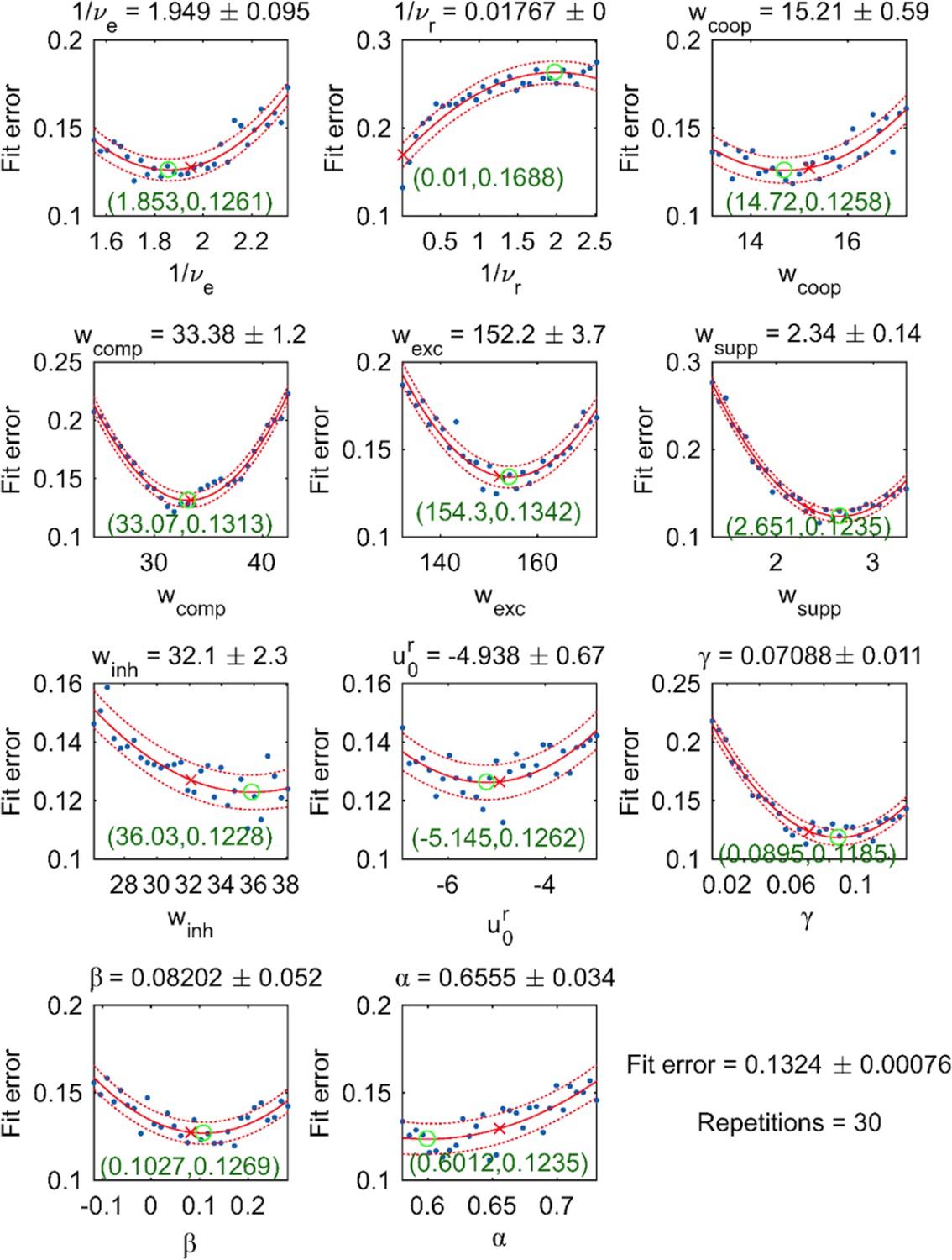
Dependence of fit error on individual parameter values (with all other parameter values fixed).

30 equally spaced values were tested (blue dots) and fitted by a quadratic function (red solid curve, with 95% confidence intervals indicated by dotted curves). For each parameter, both the optimal value (red cross) and the extremum of the parabolic fit (green circle) are shown.

Download links

A two-part list of links to download the article, or parts of the article, in various formats.

Downloads (link to download the article as PDF)

Article PDF

Open citations (links to open the citations from this article in various online reference manager services)

Mendeley

Cite this article (links to download the citations from this article in formats compatible with various reference manager tools)

Robin Cao
Alexander Pastukhov
Stepan Aleshin
Maurizio Mattia
Jochen Braun

(2021)

Binocular rivalry reveals an out-of-equilibrium neural dynamics suited for decision-making

eLife 10:e61581.

https://doi.org/10.7554/eLife.61581

Sign up for email alerts

Privacy notice