A framework for studying behavioral evolution by reconstructing ancestral repertoires
Figures
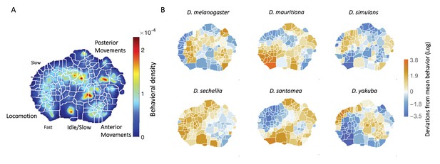
Behavioral repertoires of Drosophila.
(A) The behavioral space probability density function, obtained using the unsupervised approach described in Berman et al., 2014 on the entire data set of 561 individuals across all species. Coarse grained behaviors corresponding to the different types of movements exhibited in the map are shown as well. (B) The relative performance of each of the 134 stereotyped behaviors for each of the six species. Each region here represents a behavior, and the color scale indicates the logarithm of the fraction of time that each species performs the specified behavior divided by the average across all species.
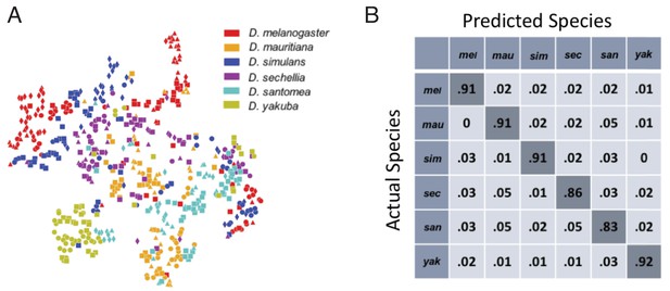
Classification of fly species based on behavioral repertoires.
(A) A t-SNE embedding of the behavioral repertoires shows that behavioral repertoires contain some species-specific information. Each dot represents one individual fly, with different colors representing different species and different symbols with the same color representing different strains within the same species. The distance matrix (561 by 561) used to create the embedding is the Jensen-Shannon divergence between the behavioral densities of individual flies. (B) Confusion matrix for the logistic regression with each row normalized. All the values are averaged from 100 different trials. The standard error is less than 0.01 for the diagonal elements and less than 0.005 for each of the off-diagonal elements.
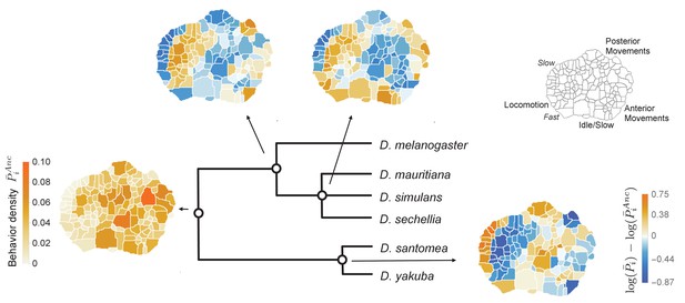
Reconstructed behavioral repertoires using the GLMM.
Inferred probabilities of the behavioral traits for the ancestral states are plotted at the denoted locations along the phylogeny. Except for the common ancestor, ancestral states are plotted with respect to the closest ancestor. For each behavioral trait, , in the intermediate ancestors, we show: , where and correspond to the inferred mean behavioral trait for the given ancestor and its closest ancestor, respectively. Coarse grained behaviors corresponding to different types of movements are shown on the top right corner.

Gelman Rubin diagnostic for model parameters inferred using MCMC.
(A) Potential Scale Reduction Factor (PSRF, see Materials and methods) for the 134 ancestral behaviors inferred in the GLMM. 20 MCMC chains with different initial conditions were used. (B) PSRF for the phylogenetic covariance matrix elements corresponding to the 10% most common behaviors performed by the measured flies. (C) PSRF for the individual covariance matrix elements corresponding to the 10% most common behaviors performed by the measured flies. The PSRF values for all of these inferred parameters indicate that the MCMC chains have converged.
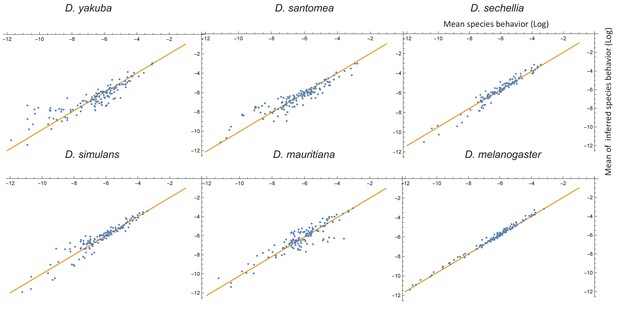
Comparison between measured and inferred behaviors (on a log scale) for each of the extant species.
Here, each measured behavioral mean plotted against the mean obtained from the components of the MCMC samples corresponding to that particular species and behavioral mode (i.e., the inferred behavioral repertories from the GLMM). The biggest differences occur mostly in the low probability behaviors, which we expect to be more sensitive to sampling errors.
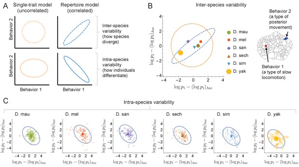
Comparison of the independent focused trait approach vs the repertoire approach for a pair of behaviors.
(A) Schematic of the different predictions that each model provides for the probability contour lines for a pair of behaviors – uncorrelated single-trait model in orange vs. correlated full-repertoire approach in blue. By definition, the single-trait model cannot predict behavioral covariance either inter- or intra-species. (B) Behavioral traits averaged within-species (colored dots) for two specific behaviors show a positive correlation, which is explained by the full-repertoire model (in blue). Ellipses are centered at the coordinates representing the behavioral traits of the inferred ancestral state, with semi-major and semi-minor axes corresponding to the eigenvectors and values of the phylogenetic covariance matrix, restricted to the behaviors shown on the left. For comparison, the contour line inferred using the single-trait model is shown in orange (level curves at two standard deviations from the mean). (C) Behavioral traits for all individuals within a species show a negative correlation, for this particular pair of behaviors, in contrast to the positive correlation observed in the species means and predicted by the full model. Blue ellipses correspond to the contour probability levels coming from the individual covariance matrix of the full-repertoire model. Note that the predictions from the single-trait model must necessarily be uncorrelated.
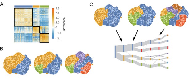
The structure of variability between flies of the same species relates to long timescale transitions in behavior.
(A) The intra-species behavioral covariance matrix (), with columns and rows ordered via an information-based clustering algorithm (Slonim et al., 2005). The black squares represent behaviors that are grouped together in the three-cluster solution. (B) Behavioral map representation of the clustering solutions. The two-, three-, and six-cluster solutions are shown on top (colors on the three cluster solution match those above the plot in A). The clusters are all spatially contiguous and break down hierarchically (see Figure 4—figure supplement 1 for more examples). (C) Clustering structure of the behavioral space obtained finding the optimally predictive groups of behaviors (see text for details). Note how these clusterings are very similar to the clusterings in B, despite having been derived from an entirely independent measure.
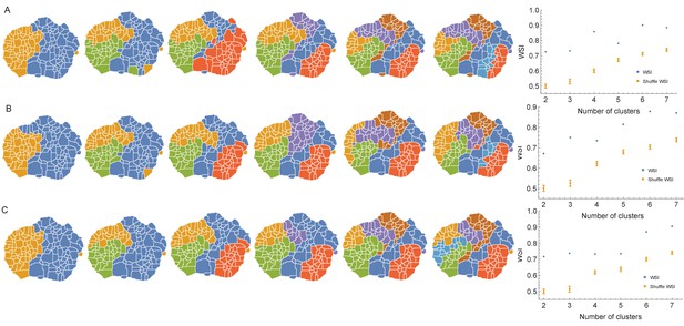
Behaviors clustered according to the individual covariance matrix using three different clustering methods.
(A) Results using k-medoids clustering method with distance matrix for 2,3,.7 clusters. To the right, the WSI between the clusters obtained using k-medoids and those obtained using the Deterministic Information Bottleneck (DIB) method on behavioral transitions (see Materials and methods). There is a high degree of similarity between these independently derived measurements, as can be shown when compared to the WSI calculated by randomly shuffling the labels of the k-medoids clustering corresponding to each number of clusters. (B) Same as in A but using Spectral clustering instead of k-medoids. The similarity index between Spectral clustering and predictive information bottleneck is also statistically significant. (C) Same as in A but using an Information-based clustering approach (see Materials and methods) instead of k-medoids. The similarity index between Information-based clustering and the results from the DIB analysis is statistically significant as well.
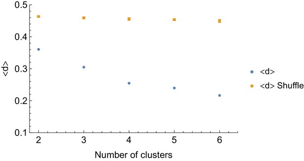
Modularity of the intra-species behavioral covariance matrix using information based clustering.
corresponds to the average distance among elements of the same clusters, (see Materials and methods). We show that for different numbers of clusters, the within-cluster distance is significantly smaller (in blue) than expected by random assignation of behaviors to clusters (in orange).
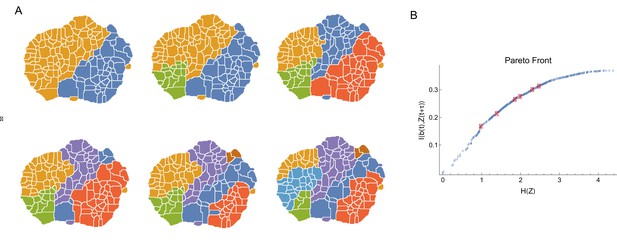
Coarse-grained behavioral representations that are optimally predictive of the future behavior states via DIB.
(A) Behavioral representation with 2,3,…,7 clusters using in Equation 10. (B) Optimal trade-off curve (Pareto Front) between complexity of coarse grained description against predictive power. For each number of clusters, representations in A correspond to points (red points) on this curve with the highest predictive information.
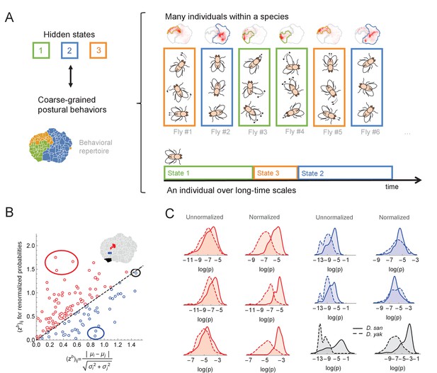
Variability within a species, long timescale transitions, and hidden states modulating behavior.
(A) A cartoon of the hypothesized relation between individual variability within a species and long timescale transitions through hidden states. (B) Accounting for the long timescale dynamics - by adjusting for the amount of time spent in each coarse-grained region (here, the six cluster solution at the top right of Figure 4C) - affects the measured behavioral distributions between D. santomea and D. yakuba. Shown is the comparison of the Mahalanobis distance () between behavioral distributions before (x-axis) and after (y-axis) adjusting. (C) Kernel density estimates of the distributions for the circled behaviors in (B) on the left before (left) and after (right) adjustments. Solid lines represent D. santomea and dashed lines represent D. yakuba.
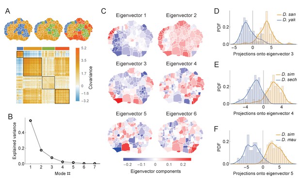
Phylogenetic variability and behavioral meta-traits.
(A) (top) Clustering the phylogenetic covariance matrix (using the same information-based clustering method from Figure 4), we observe that the clusters are no longer spatially contiguous. (bottom) The phylogenetic covariance matrix reordered according to four clusters (colors corresponding to the four-cluster map above). (B) Fraction of variance explained by the largest eigenvalues of the phylogenetic covariance matrix. (C) The eigenvectors corresponding to the largest six eigenvalues. (D) Distributions of the projections of individual density vectors from D. santomea and D. yakuba onto eigenvector 3. (E) Same as in D but using projections of individuals from D. sechellia and D. simulans onto eigenvector 4. (F) Same as in D but using projections of individuals from D. simulans and D. mauritiana onto eigenvector 5.
Additional files
-
Source data 1
Fly behavior source data.
- https://cdn.elifesciences.org/articles/61806/elife-61806-data1-v2.zip
-
Transparent reporting form
- https://cdn.elifesciences.org/articles/61806/elife-61806-transrepform-v2.docx


