Reproducible analysis of disease space via principal components using the novel R package syndRomics
- Weill Institute for Neurosciences, Brain and Spinal Injury Center (BASIC), University of California, San Francisco (UCSF), United States
- Department of Neurological Surgery, University of California San Francisco (UCSF), United States
- Zuckerberg San Francisco General Hospital and Trauma Center, United States
- School of Medicine, University of California San Diego (UCSD), United States
- San Francisco VA Health Care System, United States
Figures
Figure 1

Summary of the syndromic framework and analysis steps.
(A) The theoretical framework of syndromic analysis. The intersection between different outcome measures can create a multivariate measure (principal component if PCA is used) to explain different patterns of variance in the data. The conceptual union of three van diagram forms the core of the syndromic plot symbolizing the multidimensional measure. (B) The different steps of the workflow to using PCA such as for disease pattern analysis.
Figure 2
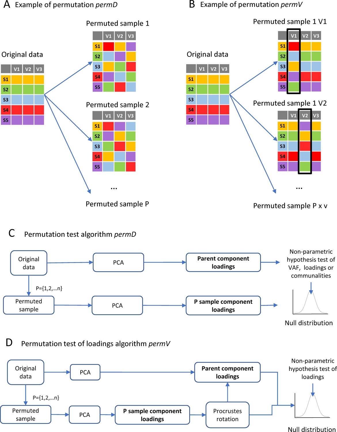
Implementation of permutation algorithms.
(A) Shows a schematic example of the permutation procedure permD where all the variables are permuted concomitantly but independently. (B) Shows a schematic example of the permutation procedure permV where variables are permuted one at the time for each permutation samples (P), keeping the other variables as in the original dataset. (C) The implemented algorithm for the permutation test algorithm using permD: each one to n permutation sample (P) consist on a random reorganization of observations inside each variable independently and concomitantly for each variable. For each P sample, a PCA is run and either the loadings, communalities or VAF are calculated. All P PCA solutions form the null distribution for non-parametric hypothesis testing of loadings or VAF. (D) The permutation test algorithm for loadings under permV is performed with and extra step of Procrustes rotation between each of the P samples to the parent component loadings. The P rotated loadings will then form the null distribution for each variable.
Figure 3 with 1 supplement
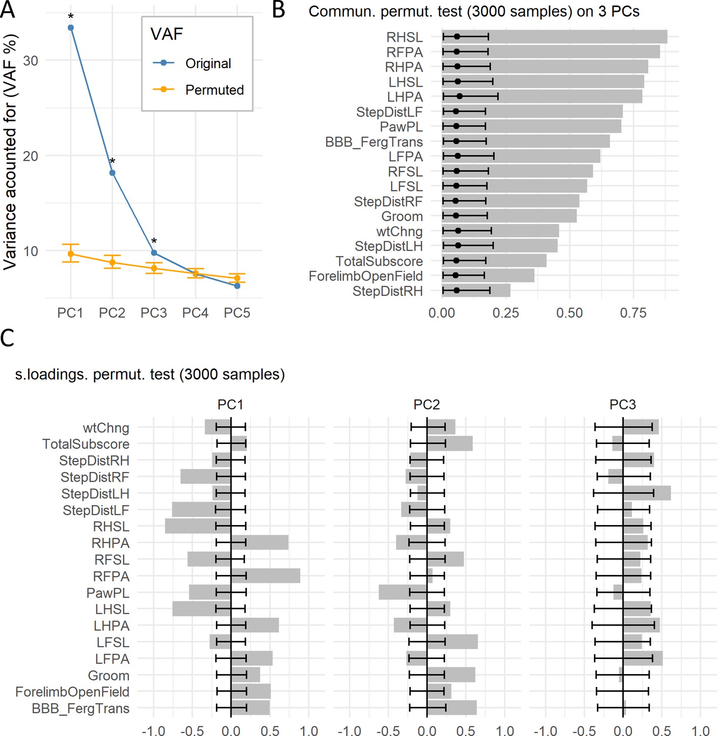
Permutation test of case study.
(A) The graph shows the original VAF for the first five PCs and the average and 95% confidence interval VAF of the permuted PCA distribution (p=10000) using the permD method. * Statistical difference for the non-parametric test at alpha = 0.05 and adjusted p value by BH. The three first PCs were selected for the subsequent analysis. (B) Barmap of the original communalities (bars) and the permuted distribution (permV, p=3000) for each variable calculated over the first three PCs. (C) Barmap of the original loadings (bars) and the permuted distribution (permV, p=3000) for each variable and each of the first three PCs. Solid dotes represent the mean of the permuted distribution and error bars represent the 95% CI.
-
Figure 3—source data 1
csv file containing the source data for panel A in Figure 3.
- https://cdn.elifesciences.org/articles/61812/elife-61812-fig3-data1-v2.csv
-
Figure 3—source data 2
csv file containing the source data for panel B in Figure 3.
- https://cdn.elifesciences.org/articles/61812/elife-61812-fig3-data2-v2.csv
-
Figure 3—source data 3
csv file containing the source data for panel C in Figure 3.
- https://cdn.elifesciences.org/articles/61812/elife-61812-fig3-data3-v2.csv
Figure 3—figure supplement 1
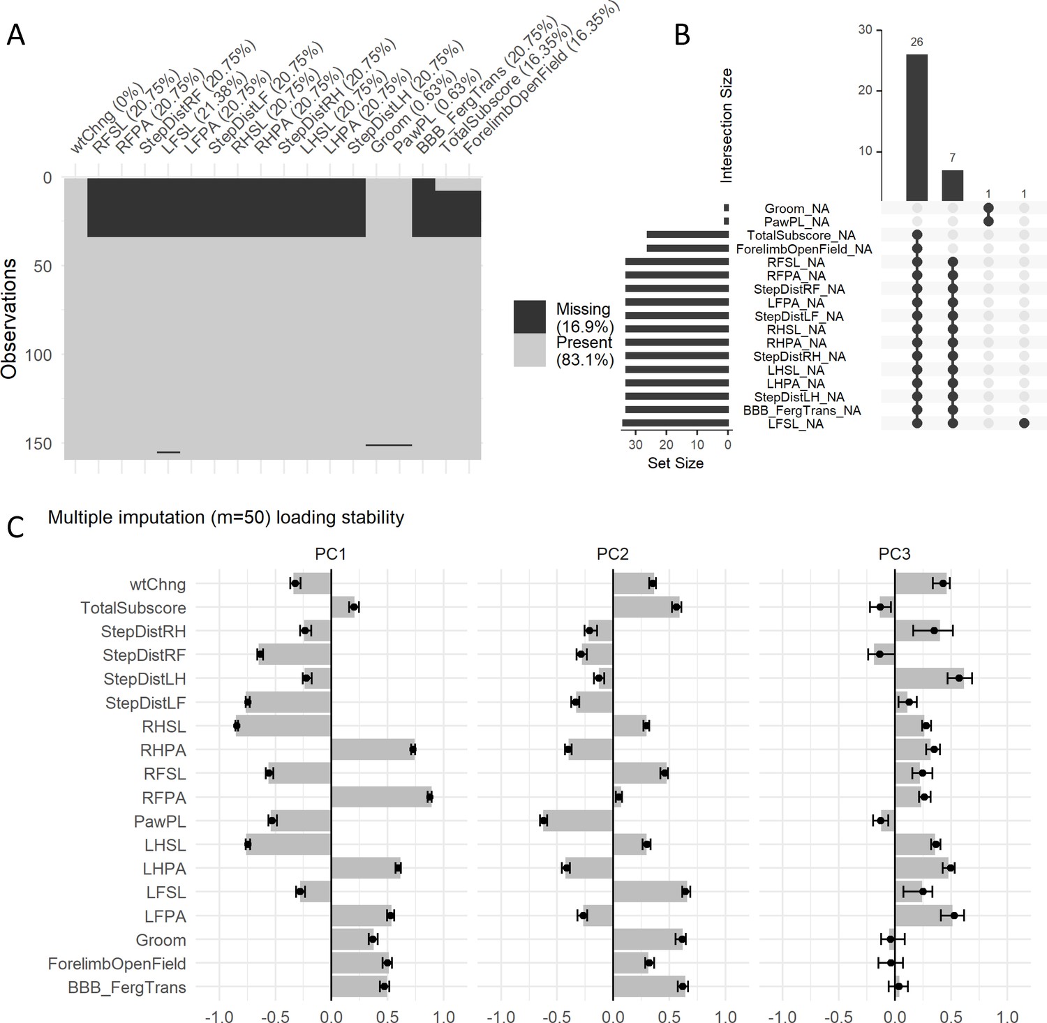
Missing data analysis of the first case study.
(A) Shadow plot of missing data for the variables selected for the case study. Approximately 17% are missing values. Four patterns of missingness are observed as shown by the upset plot (B), three patterns with involving more than one variable and a pattern with a single variable. The fact that most missing values are across variables for the same subject (two biggest missing pattern sets) suggest data is missing at random (MAR), meaning there is an external reason to the observed values for that missing. In order to assess the stability of the PCA analysis by performing multiple imputation, we calculated the distribution of loadings generated by 50 multiple imputed datasets (C). The small variation around a pooled loading (average, bar) suggest a very small variation introduced by imputing the data, further corroborated by the component similarity measures for the first three PCs (Tables 4–6). Solid dots represent the mean of the multiple imputed loading distribution and error bars represent the 95% CI.
-
Figure 3—figure supplement 1—source data 1
csv file for the Figure 3—figure supplement 1.
- https://cdn.elifesciences.org/articles/61812/elife-61812-fig3-figsupp1-data1-v2.csv
Figure 4 with 1 supplement
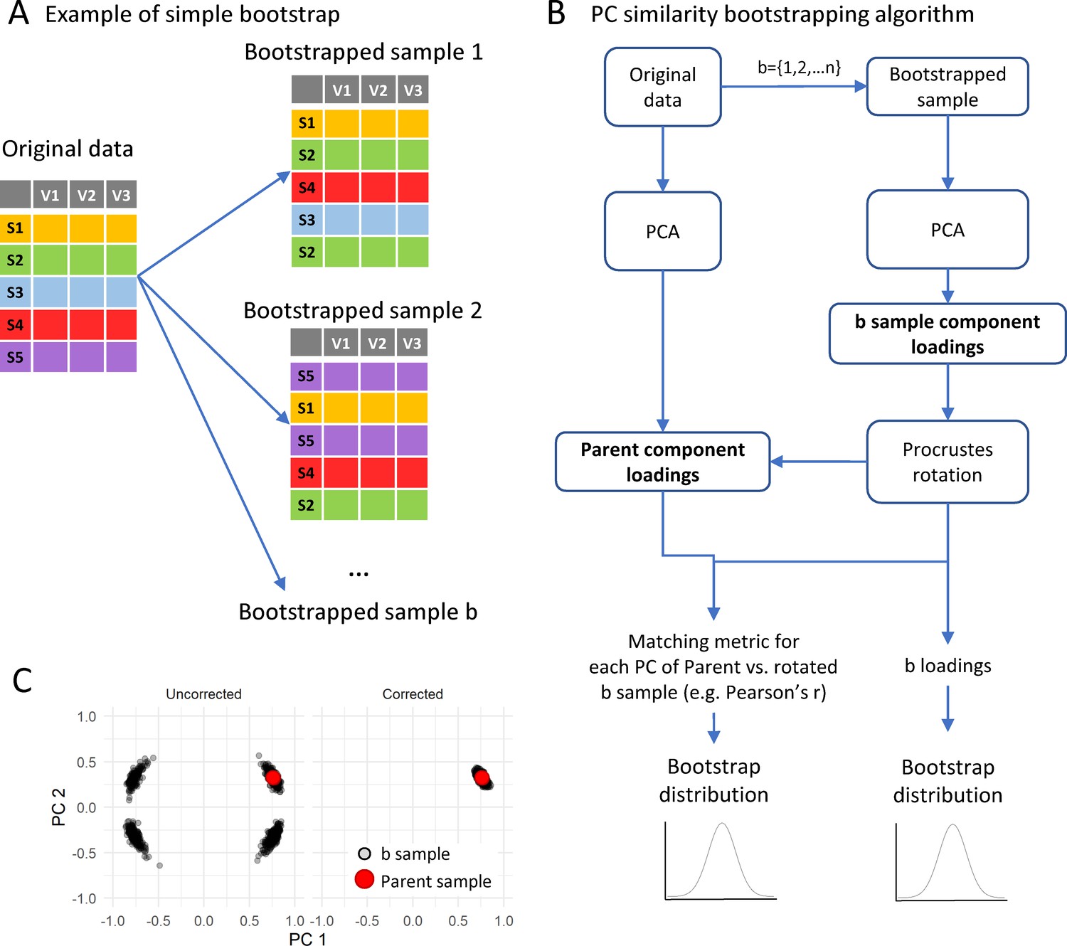
Implementation of bootstrapping algorithm.
(A) shows a schematic of the bootstrapping procedure where a bootstrap sample is generated by resampling the original samples as many times as there are samples in the original dataset but allowing for replacement. The bootstrapping algorithm for loadings is (B): for each of 1 to n bootstrap sample (b), run a PCA with the same specifications than the parent PCA on the original sample. The bootstrapping method (e.g. balanced bootstrap) can be specified with the sim argument passed to the boot() function of the boot R package. Then, the sample component loading is obtained from the PCA of the bootstrapped sample and a Procrustes rotation of the loading matrix is applied over the parent loading matrix to correct for PCA indeterminacies (C; see text). All b rotated loadings form the bootstrapped distribution of loadings. The component similarity of each b loading with the parent loading solution can be calculated to generate the bootstrapped distribution of component similarity. From these distributions, the average and confidence interval are estimated.
Figure 4—figure supplement 1
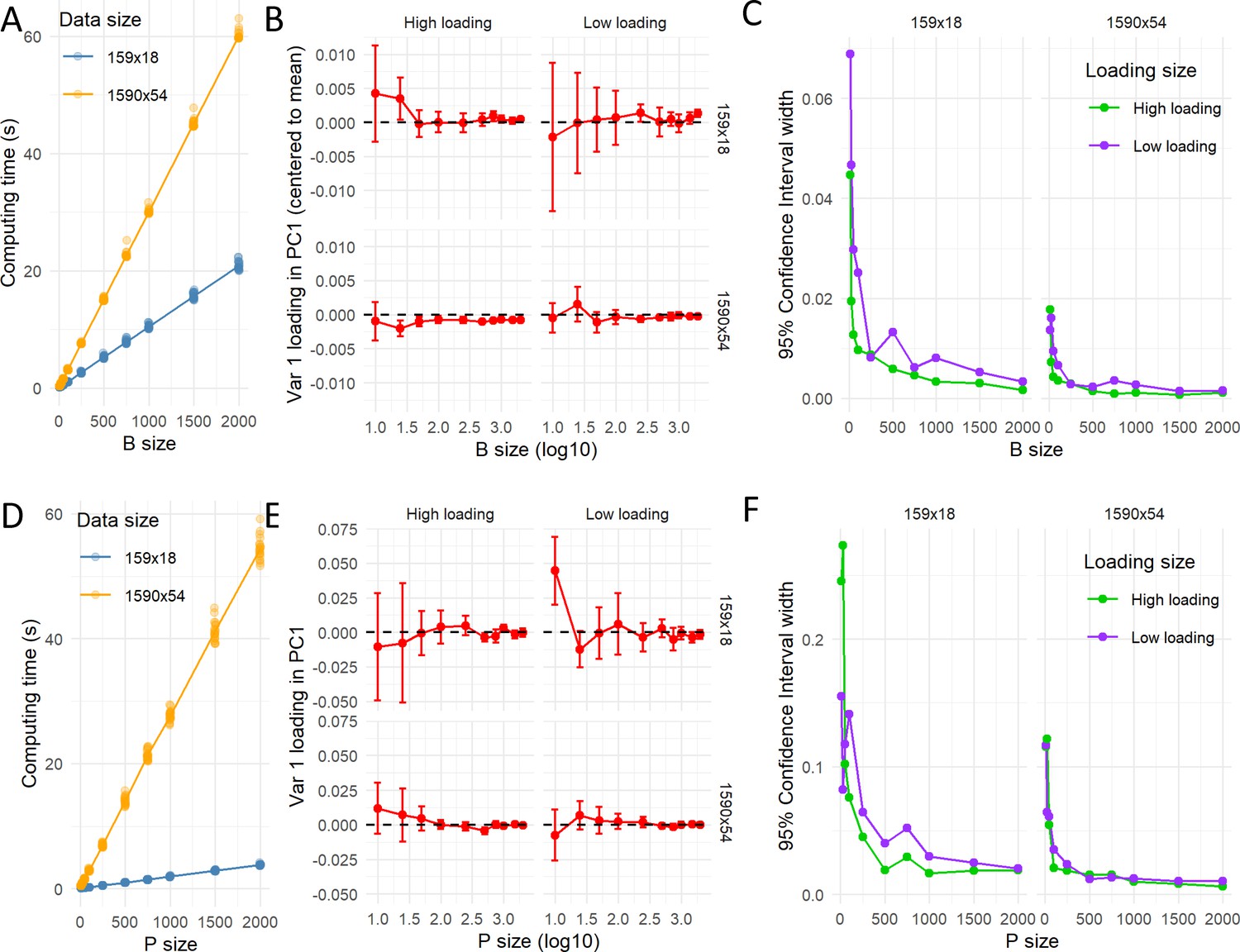
Computation time for resampling.
The pc_stability() and permut_pca_test() functions were run 10 times for different number of bootstrapped (A–C) and permuted (D–F) samples (10, 25, 50, 100, 250, 500, 750, 1000, 1500, or 2000) for two datasets with different sizes (n:rows x p:columns; 159 × 18 or 1590 × 54). The computation time (in seconds) increased linearly with the increase of samples, being the rate of increasement higher for the bigger dataset (A and D). The small margin of error for each condition (standard deviation) reflects the little effect of different runs (with different random generated numbers) on the computation time. The computed loading for a variable with high loading (~|0.75|) and another for low loading (~|0.25|) of the PC1 for each condition is shown in (B and E). As the sample size increases, the variability around the loading average decreases. The width of the 95% CI (based on t-distribution with 9 degrees of freedom) for each condition is shown (C and F) as measure of precision around the loading average estimate. The precision is smaller with the smaller size of the data, indicating that the uncertainty of the estimated averaged loading is affected by the data volume. The standard 1000 samples are a good compromise between computation time and precision of the estimated loadings for the big dataset, but smaller dataset might require bigger resamples.
Figure 5

Principal component (PC) stability results of case study.
Barmap plot of the bootstrap distribution of loadings (A) and communalities (B) representing the average and the 95% confidence interval of 3000 bootstrapped samples for the first three PCs. Assessing the confidence region offers an indicator of the uncertainty of the estimated loadings for each variable on each PC. Solid dots represent the mean of the bootstrap distribution and error bars represent the 95% CI.
Figure 6
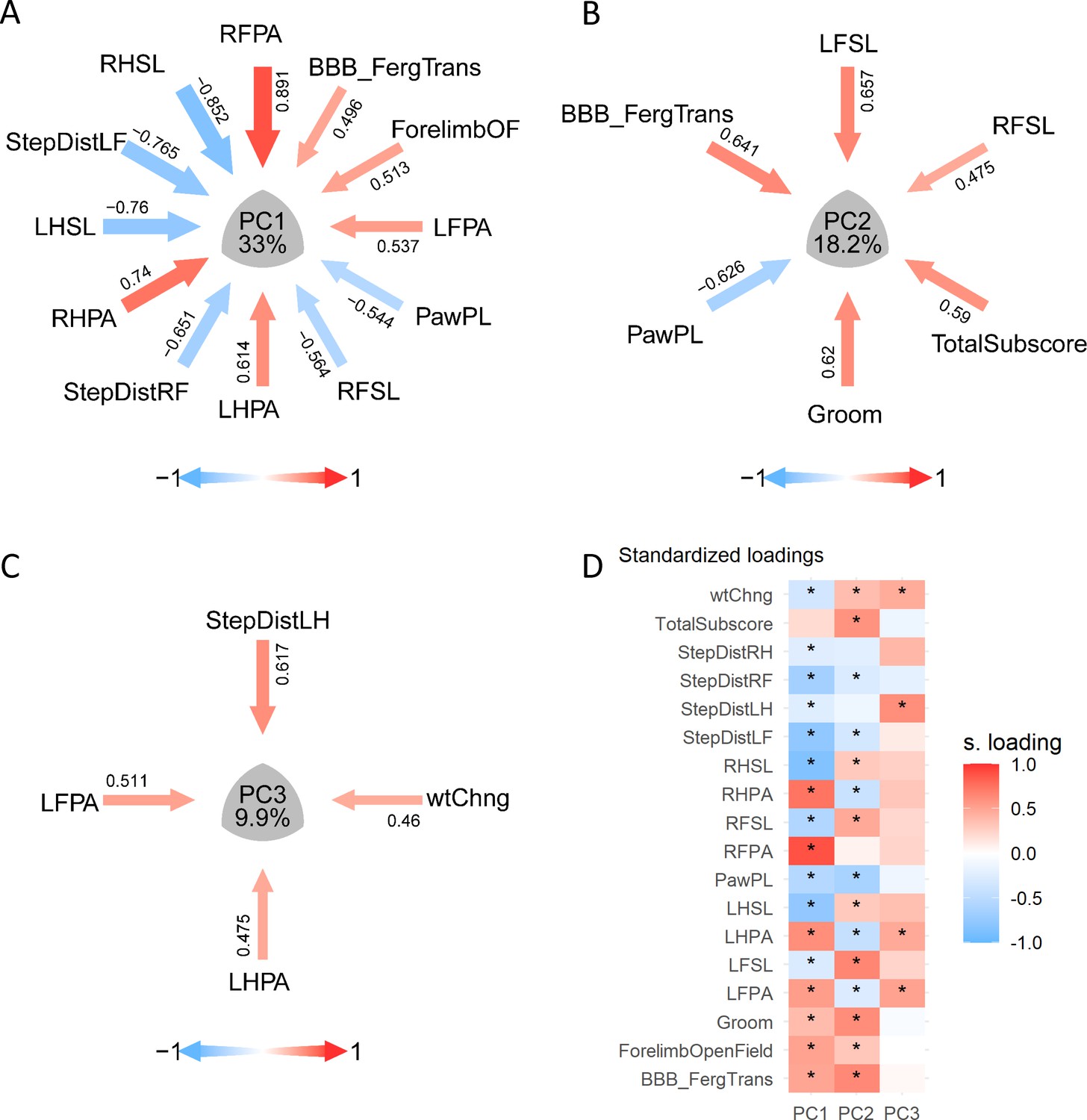
Visualization of PCA solutions for syndromic analysis.
(A–C) show the layout of the PC1, PC2, and PC3 syndromic plot of variables |loadings| > 0.45, respectively: arrows pointing the center of the plot representing the magnitude (arrow thickness and color saturation) and direction (color) of the loadings of selected variables. (D) illustrate an example of the same loading solution plotted by a heatmap. * Indicates variables with |loadings| > 0.21, 0.25 or 0.4 for PC1, PC2, and PC3, respectively.
Figure 7 with 1 supplement
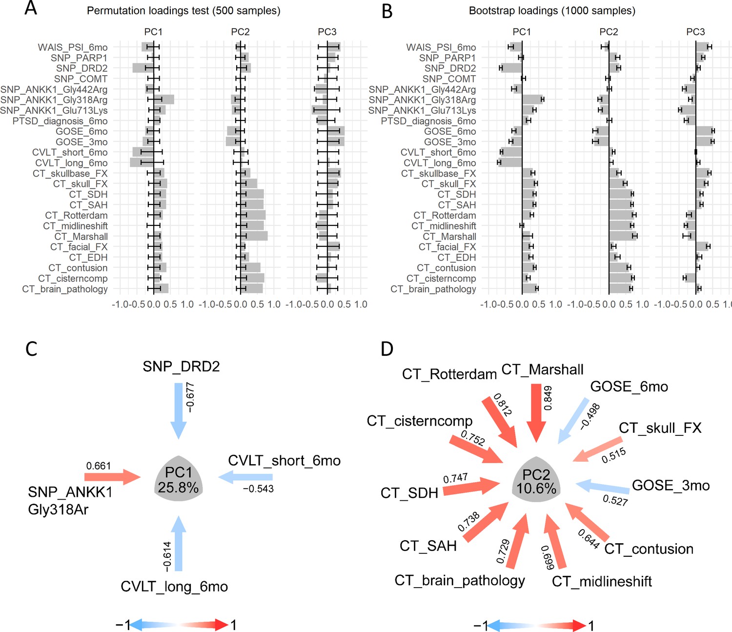
Analysis of case study 2 using non-linear PCA and the syndRomics package.
(A-B) show thebarmap plots for the loadings for the first three PCs with the 95% CI generated from 500 permutationand 1000 bootstrap resamples. (C-D) show the syndromic plots for the PC1 (VAF=25.8%) and PC2(VAF=10.6%) for |loading|>0.4. Error bars represent the 95%CI of the resampling method.
-
Figure 7—source data 1
csv file containing the source data for Figure 7.
- https://cdn.elifesciences.org/articles/61812/elife-61812-fig7-data1-v2.csv
Figure 7—figure supplement 1
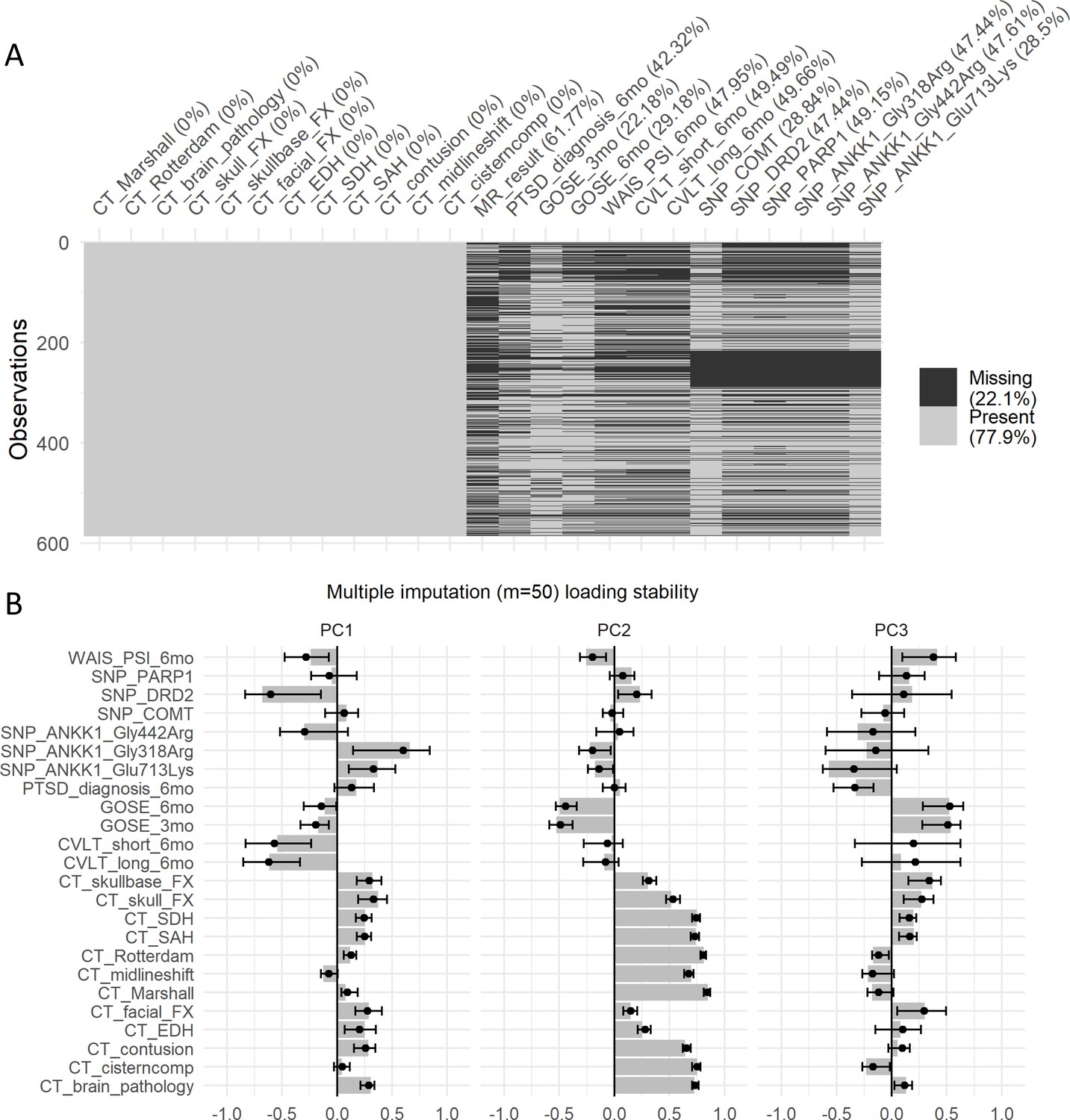
Missing data analysis of the second case study.
(A) Shadow plot of missing data for the variables selected for the case study. Approximately 22% are missing values. The fact that most missing values are across variables for the same subject (two biggest missing pattern sets) suggest data is missing at random (MAR), meaning there is an external reason to the observed values for that missing. In order to assess the stability of the PCA analysis by performing multiple imputation, we calculated the distribution of loadings generated by 50 multiple imputed datasets (B). Solid dots represent the mean of the multiple imputed loading distribution and error bars represent the 95% CI.
-
Figure 7—figure supplement 1—source data 1
csv file containing the source data for Figure 7—figure supplement 1.
- https://cdn.elifesciences.org/articles/61812/elife-61812-fig7-figsupp1-data1-v2.csv
Tables
Table 1
List of variables included in the first case study.
| Variable | Definition |
|---|---|
| wtChng | Change of animal weight (grams) from day of Injury to 6 weeks post-injury |
| RFSL | CATWALK SYSTEM RightForelimb StrideLength at 6 weeks post-injury |
| LFSL | CATWALK SYSTEM LeftForelimb StrideLength at 6 weeks post-injury |
| RHSL | CATWALK SYSTEM RightHindlimb StrideLength at 6 weeks post-injury |
| LHSL | CATWALK SYSTEM LeftHindlimb StrideLength at 6 weeks post-injury |
| RFPA | CATWALK SYSTEM RightForelimb PrintArea at 6 weeks post-injury |
| LFPA | CATWALK SYSTEM LeftForelimb PrintArea at 6 weeks post-injury |
| RHPA | CATWALK SYSTEM RightHindlimb PrintArea at 6 weeks post-injury |
| LHPA | CATWALK SYSTEM LeftHindlimb PrintArea at 6 weeks post-injury |
| StepDistRF | CATWALK SYSTEM RightForelimb Step Distribution Deviation from 25% at 6 weeks post-injury |
| StepDistLF | CATWALK SYSTEM LeftForelimb Step Distribution Deviation from 25% at 6 weeks post-injury |
| StepDistRH | CATWALK SYSTEM RightHindlimb Step Distribution Deviation from 25% at 6 weeks post-injury |
| StepDistLH | CATWALK SYSTEM LeftHindlimb Step Distribution Deviation from 25% at 6 weeks post-injury |
| TotalSubscore | Total BBB Subscore at 6 weeks post-injury |
| BBB FergTrans | BBB Ferguson Transformation score 6 weeks post-injury |
| Groom | Grooming Score 6 weeks post-injury |
| PawPL | PawPlacement score 6 weeks post-injury |
| ForelimbOpenField | Forelimb openfield score at 6 weeks post-injury |
Table 2
List of variables included in the second case study.
| Variable | Description | Values |
|---|---|---|
| CT_Marshall | Marshall CT Score | Range from 1 to 6 |
| CT_Rotterdam | Rotterdam CT Score | Range from 1 to 6 |
| CT_brain_pathology | CT Brain Pathology | 0 = ‘No’, 1 = ‘Yes’ |
| CT_skull_FX | CT Skull Fracture | 0 = ‘No’, 1 = ‘Yes’ |
| CT_skullbase_FX | CT Skull Base Fracture | 0 = ‘No’, 1 = ‘Yes’ |
| CT_facial_FX | CT Facial Fracture | 0 = ‘No’, 1 = ‘Yes’ |
| CT_EDH | CT Epidural Hematoma | 0 = ‘No’, 1 = ‘Yes’ |
| CT_SDH | CT Subdural Hematoma | 0 = ‘No’, 1 = ‘Yes’ |
| CT_SAH | CT Subarachnoid Hemorrhage | 0 = ‘No’, 1 = ‘Yes’ |
| CT_contusion | CT Contusion | 0 = ‘No’, 1 = ‘Yes’ |
| CT_midlineshift | CT Midline Shift | 0 = ‘No’, 1 = ‘Yes’ |
| CT_cisterncomp | CT Cisternal Compression | 0 = ‘No’, 1 = ‘Yes’ |
| PTSD_diagnosis_6mo | PTSD DSM-IV Diagnosis (6 months) | 0 = ‘No’, 1 = ‘Yes’ |
| GOSE_3mo | GOSE Score (3 months) | Range from 1 to 8 |
| GOSE_6mo | GOSE Score (6 months) | Range from 1 to 8 |
| WAIS_PSI_6mo | WAIS PSI Composite Score (6 months) | Range from 50 to 150 |
| CVLT_short_6mo | CVLT Short Delay Cued Recall Standard Score (6 months) | Range from −4.0–2.5 |
| CVLT_long_6mo | CVLT Long Delay Cued Recall Standard Score (6 months) | Range from −3.5–2.5 |
| SNP_COMT | COMT SNP Genotype | 1 = ‘Met/Met’, 2 = ‘Met/Val’, 3 = ‘Val/Val’ |
| SNP_DRD2 | DRD2 SNP Genotype | 1 = ‘C/C’, 2 = ‘C/T’, 3 = ‘T/T’ |
| SNP_PARP1 | PARP1 SNP Genotype | 1 = ‘A/A’, 2 = ‘A/T’, 3 = ‘T/T’ |
| SNP_ANKK1_Gly318Arg | ANKK1 SNP Gly318Arg | 1 = ‘A/A’, 2 = ‘A/G’, 3 = ‘G/G’ |
| SNP_ANKK1_Gly442Arg | ANKK1 SNP Gly442Arg | 1 = ‘C/C’, 2 = ‘C/G’, 3 = ‘G/G’ |
| SNP_ANKK1_Glu713Lys | ANKK1 SNP Glu713Lys | 1 = ‘C/C’, 2 = ‘C/T’, 3 = ‘T/T’ |
Table 3
Communalities of first three PCs on permutation test with 3000 random permutations using permV and adjusting p values with BH.
| Variable | Original communalities | Permuted average | Lower 95% CI | Upper 95% CI | p value | Adjusted p value |
|---|---|---|---|---|---|---|
| wtChng | 0.46 | 0.06 | 0.01 | 0.20 | 0.0003 | 0.0004 |
| RFSL | 0.59 | 0.06 | 0.00 | 0.20 | 0.0003 | 0.0004 |
| RFPA | 0.85 | 0.06 | 0.00 | 0.17 | 0.0003 | 0.0004 |
| StepDistRF | 0.54 | 0.05 | 0.00 | 0.17 | 0.0003 | 0.0004 |
| LFSL | 0.57 | 0.06 | 0.00 | 0.18 | 0.0003 | 0.0004 |
| LFPA | 0.61 | 0.06 | 0.00 | 0.20 | 0.0003 | 0.0004 |
| StepDistLF | 0.71 | 0.05 | 0.00 | 0.17 | 0.0003 | 0.0004 |
| RHSL | 0.88 | 0.06 | 0.00 | 0.18 | 0.0003 | 0.0004 |
| RHPA | 0.81 | 0.06 | 0.00 | 0.19 | 0.0003 | 0.0004 |
| StepDistRH | 0.27 | 0.06 | 0.00 | 0.18 | 0.0020 | 0.0020 |
| LHSL | 0.79 | 0.06 | 0.00 | 0.20 | 0.0003 | 0.0004 |
| LHPA | 0.79 | 0.07 | 0.00 | 0.23 | 0.0003 | 0.0004 |
| StepDistLH | 0.46 | 0.06 | 0.00 | 0.20 | 0.0003 | 0.0004 |
| Groom | 0.53 | 0.06 | 0.00 | 0.17 | 0.0003 | 0.0004 |
| PawPL | 0.70 | 0.06 | 0.00 | 0.17 | 0.0003 | 0.0004 |
| BBB_FergTrans | 0.66 | 0.05 | 0.00 | 0.17 | 0.0003 | 0.0004 |
| TotalSubscore | 0.40 | 0.05 | 0.00 | 0.17 | 0.0003 | 0.0004 |
| ForelimbOpenField | 0.37 | 0.05 | 0.00 | 0.18 | 0.0003 | 0.0004 |
Table 4
PC1 loading results of permutation test for the first case study with 3000 random permutations using permV and adjusting p values with BH.
| Variable | Original loading | Permuted average | Lower 95% CI | Upper 95% CI | p value | Adjusted p value |
|---|---|---|---|---|---|---|
| wtChng | −0.34 | 0.00 | −0.19 | 0.18 | 0.0003 | 0.0007 |
| TotalSubscore | −0.56 | 0.00 | −0.21 | 0.19 | 0.0003 | 0.0007 |
| StepDistRH | 0.89 | 0.01 | −0.20 | 0.21 | 0.0003 | 0.0007 |
| StepDistRF | −0.65 | 0.00 | −0.19 | 0.17 | 0.0003 | 0.0007 |
| StepDistLH | −0.28 | 0.00 | −0.18 | 0.18 | 0.0043 | 0.0084 |
| StepDistLF | 0.54 | 0.01 | −0.18 | 0.18 | 0.0003 | 0.0007 |
| RHSL | −0.76 | 0.00 | −0.19 | 0.19 | 0.0003 | 0.0007 |
| RHPA | −0.85 | 0.00 | −0.17 | 0.19 | 0.0003 | 0.0007 |
| RFSL | 0.74 | 0.01 | −0.18 | 0.19 | 0.0003 | 0.0007 |
| RFPA | −0.25 | 0.00 | −0.18 | 0.18 | 0.0063 | 0.0114 |
| PawPL | −0.76 | 0.00 | −0.17 | 0.17 | 0.0003 | 0.0007 |
| LHSL | 0.62 | 0.00 | −0.18 | 0.18 | 0.0003 | 0.0007 |
| LHPA | −0.24 | 0.00 | −0.19 | 0.17 | 0.0163 | 0.0259 |
| LFSL | 0.38 | 0.01 | −0.17 | 0.20 | 0.0003 | 0.0007 |
| LFPA | −0.54 | −0.01 | −0.21 | 0.20 | 0.0003 | 0.0007 |
| Groom | 0.49 | 0.00 | −0.20 | 0.19 | 0.0003 | 0.0007 |
| ForelimbOpenField | 0.20 | −0.01 | −0.19 | 0.18 | 0.0323 | 0.0459 |
| BBB_FergTrans | 0.51 | 0.01 | −0.18 | 0.19 | 0.0003 | 0.0007 |
Table 5
PC2 loading results of permutation test for the first case study with 3000 random permutations using permV and adjusting p values with BH.
| Variable | Original loading | Permuted average | Lower 95% CI | Upper 95% CI | p value | Adjusted p value |
|---|---|---|---|---|---|---|
| wtChng | −0.37 | 0.00 | −0.23 | 0.22 | 0.0023 | 0.0047 |
| TotalSubscore | −0.48 | −0.01 | −0.23 | 0.21 | 0.0003 | 0.0007 |
| StepDistRH | −0.07 | −0.01 | −0.23 | 0.23 | 0.5122 | 0.5644 |
| StepDistRF | 0.28 | 0.00 | −0.23 | 0.21 | 0.0143 | 0.0234 |
| StepDistLH | −0.66 | 0.01 | −0.23 | 0.24 | 0.0003 | 0.0007 |
| StepDistLF | 0.27 | 0.00 | −0.22 | 0.23 | 0.0203 | 0.0305 |
| RHSL | 0.34 | 0.00 | −0.24 | 0.23 | 0.0003 | 0.0007 |
| RHPA | −0.30 | 0.00 | −0.21 | 0.21 | 0.0083 | 0.0145 |
| RFSL | 0.40 | 0.00 | −0.22 | 0.25 | 0.0003 | 0.0007 |
| RFPA | 0.21 | 0.00 | −0.22 | 0.22 | 0.0643 | 0.0868 |
| PawPL | −0.30 | 0.00 | −0.19 | 0.22 | 0.0023 | 0.0047 |
| LHSL | 0.42 | 0.01 | −0.21 | 0.23 | 0.0003 | 0.0007 |
| LHPA | 0.12 | 0.00 | −0.24 | 0.22 | 0.3182 | 0.3656 |
| LFSL | −0.62 | 0.00 | −0.25 | 0.25 | 0.0003 | 0.0007 |
| LFPA | 0.63 | 0.00 | −0.24 | 0.26 | 0.0003 | 0.0007 |
| Groom | −0.65 | 0.00 | −0.22 | 0.23 | 0.0003 | 0.0007 |
| ForelimbOpenField | −0.59 | −0.01 | −0.25 | 0.23 | 0.0003 | 0.0007 |
| BBB_FergTrans | −0.32 | −0.01 | −0.22 | 0.22 | 0.0023 | 0.0047 |
Table 6
PC3 loading results of permutation test for the first case study with 3000 random permutations using permV and adjusting p values with BH.
| Variable | Original loading | Permuted average | Lower 95% CI | Upper 95% CI | p value | Adjusted p value |
|---|---|---|---|---|---|---|
| wtChng | 0.46 | 0.00 | −0.43 | 0.41 | 0.0183 | 0.0283 |
| TotalSubscore | 0.22 | 0.00 | −0.32 | 0.34 | 0.2463 | 0.2955 |
| StepDistRH | 0.23 | 0.01 | −0.32 | 0.35 | 0.2303 | 0.2826 |
| StepDistRF | −0.19 | 0.01 | −0.32 | 0.34 | 0.3102 | 0.3642 |
| StepDistLH | 0.23 | 0.00 | −0.34 | 0.36 | 0.2083 | 0.2615 |
| StepDistLF | 0.50 | −0.01 | −0.36 | 0.40 | 0.0063 | 0.0114 |
| RHSL | 0.12 | 0.00 | −0.35 | 0.33 | 0.5382 | 0.5698 |
| RHPA | 0.26 | 0.00 | −0.35 | 0.35 | 0.1903 | 0.2446 |
| RFSL | 0.32 | 0.00 | −0.36 | 0.41 | 0.1043 | 0.1374 |
| RFPA | 0.41 | 0.00 | −0.34 | 0.35 | 0.0223 | 0.0326 |
| PawPL | 0.35 | −0.01 | −0.37 | 0.35 | 0.0583 | 0.0807 |
| LHSL | 0.48 | 0.01 | −0.39 | 0.44 | 0.0123 | 0.0208 |
| LHPA | 0.62 | 0.00 | −0.38 | 0.35 | 0.0003 | 0.0007 |
| LFSL | −0.05 | 0.00 | −0.35 | 0.33 | 0.8001 | 0.8308 |
| LFPA | −0.12 | −0.01 | −0.32 | 0.34 | 0.5302 | 0.5698 |
| Groom | 0.03 | 0.01 | −0.34 | 0.34 | 0.8680 | 0.8844 |
| ForelimbOpenField | −0.14 | 0.01 | −0.32 | 0.34 | 0.4802 | 0.5402 |
| BBB_FergTrans | 0.00 | 0.02 | −0.33 | 0.33 | 0.9900 | 0.9900 |
Table 7
Similarity metrics of the first three PCs between 50 multiple imputed datasets for the first case study.
Silent cutoff for S index was set at |0.2|.
| CC index | r index | RMSE | S index | |||||
|---|---|---|---|---|---|---|---|---|
| PC | Mean | SD | Mean | SD | Mean | SD | Mean | SD |
| PC1 | 0.999 | 0.0003 | 0.999 | 0.0003 | 0.021 | 0.004 | 0.991 | 0.015 |
| PC2 | 0.998 | 0.0005 | 0.998 | 0.0005 | 0.021 | 0.004 | 0.93 | 0.042 |
| PC3 | 0.997 | 0.001 | 0.996 | 0.002 | 0.022 | 0.005 | 0.965 | 0.03 |
Table 8
PC1 loading results of permutation test for the second case study with 500 random permutations using permV and adjusting p values with BH.
| Variable | Original loading | Permuted average | Lower 95% CI | Upper 95% CI | p value | Adjusted p value |
|---|---|---|---|---|---|---|
| CT_brain_pathology | 0.440589 | 0.010978 | −0.17606 | 0.202095 | 0.001996 | 0.003194 |
| CT_cisterncomp | 0.1844 | 0.003484 | −0.16947 | 0.209801 | 0.053892 | 0.061591 |
| CT_contusion | 0.382612 | 0.008019 | −0.17053 | 0.187363 | 0.001996 | 0.003194 |
| CT_EDH | 0.256368 | 0.015695 | −0.16239 | 0.190167 | 0.001996 | 0.003194 |
| CT_facial_FX | 0.267322 | 0.029918 | −0.16465 | 0.202063 | 0.011976 | 0.015128 |
| CT_Marshall | 0.235242 | 0.003685 | −0.16912 | 0.191229 | 0.00998 | 0.013307 |
| CT_midlineshift | 0.002539 | −0.01082 | −0.2005 | 0.190956 | 0.988024 | 0.988024 |
| CT_Rotterdam | 0.274699 | 0.010723 | −0.17176 | 0.195646 | 0.001996 | 0.003194 |
| CT_SAH | 0.376596 | 0.009848 | −0.16185 | 0.191671 | 0.001996 | 0.003194 |
| CT_SDH | 0.377542 | 0.018196 | −0.15488 | 0.196538 | 0.001996 | 0.003194 |
| CT_skull_FX | 0.404447 | 0.020049 | −0.15398 | 0.198067 | 0.001996 | 0.003194 |
| CT_skullbase_FX | 0.318179 | 0.019653 | −0.18691 | 0.195547 | 0.001996 | 0.003194 |
| CVLT_long_6mo | −0.70622 | −0.05218 | −0.37582 | 0.295769 | 0.001996 | 0.003194 |
| CVLT_short_6mo | −0.63345 | −0.04306 | −0.378 | 0.258602 | 0.001996 | 0.003194 |
| GOSE_3mo | −0.32848 | −0.00894 | −0.17465 | 0.177456 | 0.001996 | 0.003194 |
| GOSE_6mo | −0.25329 | −0.00613 | −0.19298 | 0.176343 | 0.003992 | 0.005988 |
| PTSD_diagnosis_6mo | 0.188743 | 0.013079 | −0.15885 | 0.190364 | 0.041916 | 0.050299 |
| SNP_ANKK1_Glu713Lys | 0.358071 | 0.028077 | −0.14647 | 0.190965 | 0.001996 | 0.003194 |
| SNP_ANKK1_Gly318Arg | 0.613624 | 0.043104 | −0.17747 | 0.244082 | 0.001996 | 0.003194 |
| SNP_ANKK1_Gly442Arg | −0.25194 | −0.02327 | −0.19756 | 0.16577 | 0.005988 | 0.008454 |
| SNP_COMT | 0.036687 | 0.001474 | −0.17511 | 0.172543 | 0.696607 | 0.726894 |
| SNP_DRD2 | −0.62858 | −0.05017 | −0.24105 | 0.168359 | 0.001996 | 0.003194 |
| SNP_PARP1 | −0.05912 | −0.00576 | −0.18101 | 0.166475 | 0.512974 | 0.559608 |
| WAIS_PSI_6mo | −0.36179 | −0.0144 | −0.19646 | 0.168075 | 0.001996 | 0.003194 |
Table 9
PC2 loading results of permutation test for the second case study with 500 random permutations using permV and adjusting p values with BH.
| Variable | Original loading | Permuted average | Lower 95% CI | Upper 95% CI | p value | Adjusted p value |
|---|---|---|---|---|---|---|
| CT_brain_pathology | 0.662378 | 0.021655 | −0.12084 | 0.158839 | 0.001996 | 0.002818 |
| CT_cisterncomp | 0.709989 | 0.024823 | −0.14181 | 0.178126 | 0.001996 | 0.002818 |
| CT_contusion | 0.596311 | 0.01766 | −0.12222 | 0.157785 | 0.001996 | 0.002818 |
| CT_EDH | 0.253079 | 0.002735 | −0.13662 | 0.135348 | 0.001996 | 0.002818 |
| CT_facial_FX | 0.142602 | 0.000971 | −0.12466 | 0.133574 | 0.041916 | 0.055888 |
| CT_Marshall | 0.809847 | 0.026415 | −0.13438 | 0.173771 | 0.001996 | 0.002818 |
| CT_midlineshift | 0.69605 | 0.034813 | −0.12917 | 0.189917 | 0.001996 | 0.002818 |
| CT_Rotterdam | 0.753498 | 0.01539 | −0.13205 | 0.178638 | 0.001996 | 0.002818 |
| CT_SAH | 0.689084 | 0.017617 | −0.12425 | 0.155246 | 0.001996 | 0.002818 |
| CT_SDH | 0.698728 | 0.017798 | −0.12057 | 0.161901 | 0.001996 | 0.002818 |
| CT_skull_FX | 0.493199 | 0.007764 | −0.13921 | 0.161888 | 0.001996 | 0.002818 |
| CT_skullbase_FX | 0.294691 | 0.003769 | −0.12863 | 0.141375 | 0.001996 | 0.002818 |
| CVLT_long_6mo | 0.056095 | 0.019229 | −0.21544 | 0.23499 | 0.674651 | 0.703983 |
| CVLT_short_6mo | 0.115663 | 0.020014 | −0.20152 | 0.215121 | 0.353293 | 0.423952 |
| GOSE_3mo | −0.43692 | −0.00787 | −0.14301 | 0.139508 | 0.001996 | 0.002818 |
| GOSE_6mo | −0.40155 | −0.00849 | −0.14484 | 0.118386 | 0.001996 | 0.002818 |
| PTSD_diagnosis_6mo | 0.004807 | −0.00863 | −0.14863 | 0.140418 | 0.94012 | 0.94012 |
| SNP_ANKK1_Glu713Lys | −0.26204 | −0.01604 | −0.15757 | 0.132164 | 0.001996 | 0.002818 |
| SNP_ANKK1_Gly318Arg | −0.28622 | −0.01954 | −0.15986 | 0.133637 | 0.001996 | 0.002818 |
| SNP_ANKK1_Gly442Arg | 0.033308 | −0.00308 | −0.12662 | 0.129371 | 0.630739 | 0.688078 |
| SNP_COMT | −0.0406 | −0.00094 | −0.14047 | 0.140783 | 0.588822 | 0.67294 |
| SNP_DRD2 | 0.307457 | 0.023806 | −0.11549 | 0.178777 | 0.001996 | 0.002818 |
| SNP_PARP1 | 0.244246 | 0.000876 | −0.14801 | 0.133131 | 0.001996 | 0.002818 |
| WAIS_PSI_6mo | −0.13252 | 0.001279 | −0.13167 | 0.134985 | 0.055888 | 0.070596 |
Table 10
PC3 loading results of permutation test for the second case study with 500 random permutations using permV and adjusting p values with BH.
| Variable | Original loading | Permuted average | Lower 95% CI | Upper 95% CI | p value | Adjusted p value |
|---|---|---|---|---|---|---|
| CT_brain_pathology | 0.110149 | 0.002819 | −0.30242 | 0.309376 | 0.528942 | 0.641916 |
| CT_cisterncomp | −0.32449 | −0.00334 | −0.33379 | 0.305672 | 0.047904 | 0.13839 |
| CT_contusion | 0.060972 | −0.00689 | −0.31444 | 0.270176 | 0.698603 | 0.728977 |
| CT_EDH | 0.104859 | −0.00125 | −0.27352 | 0.321535 | 0.518962 | 0.641916 |
| CT_facial_FX | 0.371649 | 0.062687 | −0.31692 | 0.355691 | 0.01996 | 0.07984 |
| CT_Marshall | −0.24284 | −0.01023 | −0.3038 | 0.288171 | 0.129741 | 0.259481 |
| CT_midlineshift | −0.30562 | −0.01988 | −0.32888 | 0.308785 | 0.063872 | 0.153293 |
| CT_Rotterdam | −0.24002 | −0.01377 | −0.32884 | 0.292959 | 0.161677 | 0.284003 |
| CT_SAH | 0.16969 | −0.0017 | −0.30469 | 0.323896 | 0.347305 | 0.520958 |
| CT_SDH | 0.164146 | 0.011718 | −0.33537 | 0.308091 | 0.339321 | 0.520958 |
| CT_skull_FX | 0.30911 | 0.013422 | −0.28309 | 0.317483 | 0.047904 | 0.13839 |
| CT_skullbase_FX | 0.412507 | 0.027909 | −0.29748 | 0.350075 | 0.005988 | 0.047904 |
| CVLT_long_6mo | 0.071561 | 0.007602 | −0.26795 | 0.330045 | 0.662675 | 0.722918 |
| CVLT_short_6mo | 0.01478 | 0.003403 | −0.29415 | 0.341327 | 0.922156 | 0.922156 |
| GOSE_3mo | 0.512173 | 0.027225 | −0.3035 | 0.347452 | 0.001996 | 0.023952 |
| GOSE_6mo | 0.519654 | 0.030422 | −0.28179 | 0.361045 | 0.001996 | 0.023952 |
| PTSD_diagnosis_6mo | −0.29067 | −0.02728 | −0.31023 | 0.227907 | 0.051896 | 0.13839 |
| SNP_ANKK1_Glu713Lys | −0.47272 | −0.02347 | −0.40038 | 0.368874 | 0.007984 | 0.047904 |
| SNP_ANKK1_Gly318Arg | −0.14092 | −0.02104 | −0.34164 | 0.27799 | 0.379242 | 0.5354 |
| SNP_ANKK1_Gly442Arg | −0.34766 | −0.02656 | −0.38332 | 0.353987 | 0.083832 | 0.182907 |
| SNP_COMT | −0.10171 | 0.001249 | −0.26635 | 0.284647 | 0.53493 | 0.641916 |
| SNP_DRD2 | 0.081296 | 0.013862 | −0.2912 | 0.323114 | 0.61477 | 0.702595 |
| SNP_PARP1 | 0.233007 | 0.010172 | −0.29054 | 0.318385 | 0.165669 | 0.284003 |
| WAIS_PSI_6mo | 0.39706 | 0.017391 | −0.27022 | 0.337713 | 0.011976 | 0.057485 |
Table 11
Similarity metrics of the first 3PCs between 50 multiple imputed datasets for the second case study.
Silent cutoff for S index was set at |0.2|.
| CC index | r index | RMSE | S index | |||||
|---|---|---|---|---|---|---|---|---|
| PC | Mean | SD | Mean | SD | Mean | SD | Mean | SD |
| PC1 | 0.955 | 0.035 | 0.958 | 0.033 | 0.094 | 0.06 | 0.88 | 0.037 |
| PC2 | 0.992 | 0.004 | 0.991 | 0.0054 | 0.056 | 0.039 | 0.93 | 0.04 |
| PC3 | 0.87 | 0.097 | 0.874 | 0.097 | 0.133 | 0.127 | 0.71 | 0.06 |
Table 12
Template/example of data.frame containing loadings that can be passed to the visualization functions (only the loadings for the first three PCs are shown).
| Variable | PC1 | PC2 | PC3 |
|---|---|---|---|
| wtChng | −0.34 | −0.37 | 0.46 |
| TotalSubscore | −0.56 | −0.48 | 0.22 |
| StepDistRH | 0.89 | −0.07 | 0.23 |
| StepDistRF | −0.65 | 0.28 | −0.19 |
| StepDistLH | −0.28 | −0.66 | 0.23 |
| StepDistLF | 0.54 | 0.27 | 0.50 |
| RHSL | −0.76 | 0.34 | 0.12 |
| RHPA | −0.85 | −0.30 | 0.26 |
| RFSL | 0.74 | 0.40 | 0.32 |
| RFPA | −0.25 | 0.21 | 0.41 |
| PawPL | −0.76 | −0.30 | 0.35 |
| LHSL | 0.62 | 0.42 | 0.48 |
| LHPA | −0.24 | 0.12 | 0.62 |
| LFSL | 0.38 | −0.62 | −0.05 |
| LFPA | −0.54 | 0.63 | −0.12 |
| Groom | 0.49 | −0.65 | 0.03 |
| ForelimbOpenField | 0.20 | −0.59 | −0.14 |
| BBB_FergTrans | 0.51 | −0.32 | −0.03 |
Additional files
-
Source code 1
The R script reproducing the analysis of this manuscript in a Rmarkdown file.
- https://cdn.elifesciences.org/articles/61812/elife-61812-code1-v2.zip
-
Source code 2
A rendered script with code and outputs of running the code in a html file.
- https://cdn.elifesciences.org/articles/61812/elife-61812-code2-v2.zip
-
Transparent reporting form
- https://cdn.elifesciences.org/articles/61812/elife-61812-transrepform-v2.docx
Download links
A two-part list of links to download the article, or parts of the article, in various formats.
Downloads (link to download the article as PDF)
Open citations (links to open the citations from this article in various online reference manager services)
Cite this article (links to download the citations from this article in formats compatible with various reference manager tools)
Reproducible analysis of disease space via principal components using the novel R package syndRomics
eLife 10:e61812.
https://doi.org/10.7554/eLife.61812


