The temporal representation of experience in subjective mood
- Section of Clinical and Computational Psychiatry, National Institute of Mental Health, National Institutes of Health, United States
- Machine Learning Team, National Institute of Mental Health, National Institutes of Health, United States
- Emotion and Development Branch, National Institute of Mental Health, National Institutes of Health, United States
- Department of Psychology, Yale University, United States
- Max Planck UCL Centre for Computational Psychiatry and Ageing Research, University College London, United Kingdom
- Wellcome Centre for Human Neuroimaging, University College London, United Kingdom
Figures
Figure 1 with 1 supplement
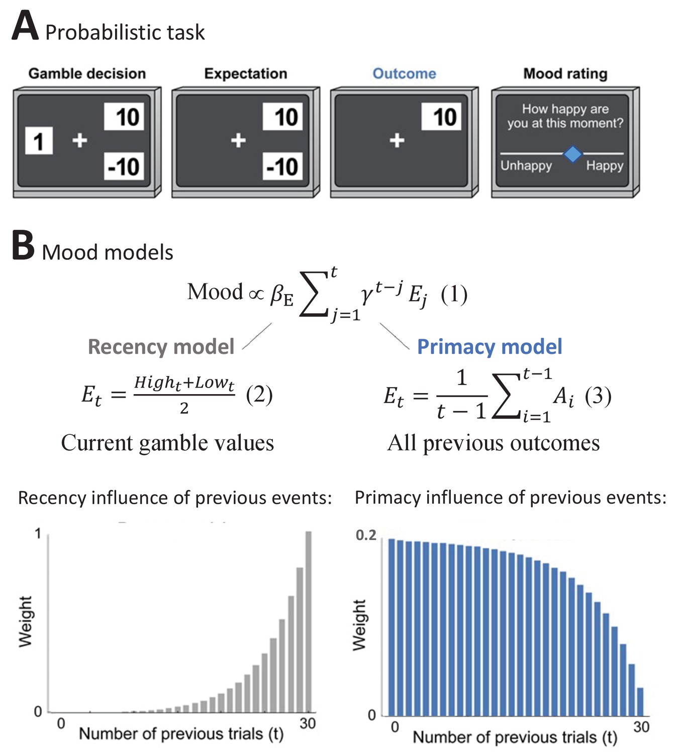
The Primacy versus Recency mood models.
(A) Participants played a probabilistic task where they experienced different reward prediction error values, while reporting subjective mood every 2-3 gambling trials. In each trial, participants chose whether to gamble between two monetary values or to receive a certain amount (Gamble decision). During Expectation, the chosen option remained on the screen, followed by the presentation of the Outcome value. (B)
(1)
presents the expectation term of the mood models, where βE is the influence of expectation values on subjective mood reports. The expectation term of the Recency mood model as developed by Rutledge et al., 2014 is presented below
(2)
where it consists of the trial’s high and low gamble values. In the alternative Primacy model, as presented in
(3)
the expectation term is replaced by the average of all previous outcomes (Ai). Moreover, as can be seen in Equations 6–8 in Materials and methods, the Primacy model has overall fewer parameters compared to the Recency model. The theoretical scaling curves for the influence of previous events on mood due to expected outcomes are presented for each model respectively below (see Figure 1—figure supplement 1 for additional illustrations).
Figure 1—figure supplement 1
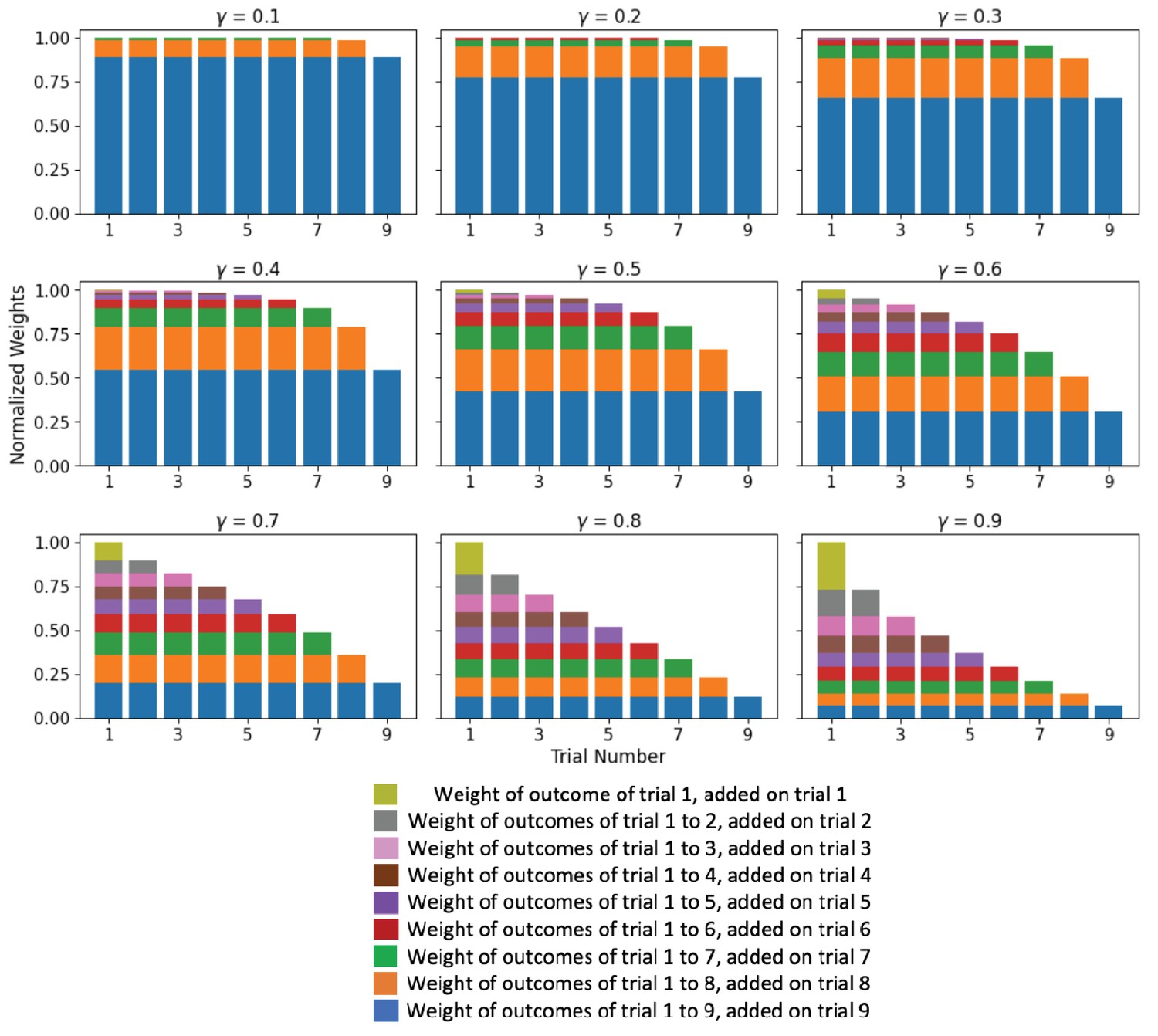
The Primacy effect of outcomes on mood.
In the Primacy model, the expectation term is the unweighted average of previous outcomes. At each trial, all previous expectation terms are combined in an exponentially weighted sum: . Here, we illustrate how this gives rise to a primacy weighting of previous outcomes that depends on the value of (each subplot represents a different magnitude of exponential weighting ). The total height of each bar represents the influence of the outcome of the corresponding trial on the result of the exponential sum at the end of trial 9. Each color indicates the contributions of the outcomes that form an expectation term at the end of trial j. The dark yellow block represents the contribution of the expectation term from the end of trial 1 (comprised only of the first outcome). The gray blocks represent the contributions of the expectation term that is being added from the end of trial 2 (which is the average of the outcomes from trials 1 and 2, and therefore it appears in both the first and the second bars). This continues for the rest of the expectation terms until the last expectation term is added, which is formed by averaging the outcomes from trials 1 to 9 as shown by the blue bars.
Figure 2

Different experimental reward environments.
(A) Reward prediction error (RPE) values received during each task version, averaged across all participants (shaded areas represent SEM). (B) The influence of RPE values on mood reports along the task, averaged across all participants (shaded areas are SEM). See Materials and methods for a link to the online repository from where the source data of this figure can be downloaded.
Figure 3 with 3 supplements
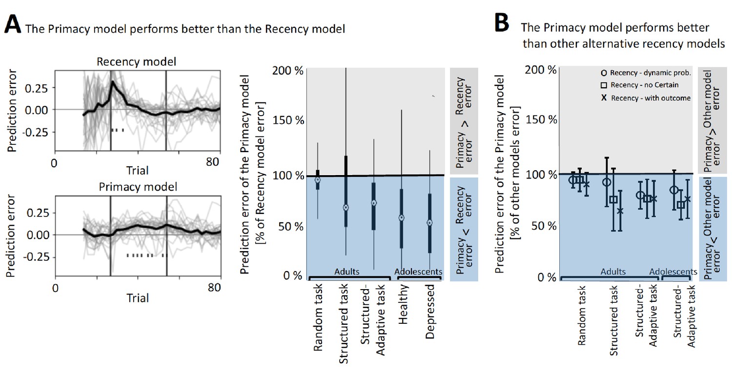
The better performance of the Primacy model.
(A) Model comparison between the Primacy and the Recency models, using the streaming prediction criterion, where the model is predicting each mood rating using the preceding ratings. On the left, the trial-level errors in predicting mood with the Recency and the Primacy models are shown for all participants, during the structure-adaptive task (bold line depicts average across all participants). This error is calculated by predicting the t-th mood rating using all preceding (1 to t-1) mood ratings, and therefore fitting iterations start only as of the fourth mood rating (~15 gambling trials), which ensures that models have sufficient data to fit all parameters. The right panel presents the median of mean squared errors (MSEs) of the Primacy model relative to the Recency model in this criterion across all datasets (edges indicate 25th and 75th percentiles, and error bars show the most extreme data point not considered an outlier). (B) Model comparison between the Primacy and three variants of the Recency model, which also shows lower MSEs for the Primacy model. Values are median MSEs of the Primacy model relative to each of the alternative models (i.e., Recency with dynamic probability model marked with circles, Recency without the Certain term model marked with squares, and the Recency with outcomes as expectation model marked by crosses), and error bars are standard deviation across participants. The values used to derive these plots are available in Table 1, fit coefficients are presented in Figure 3—figure supplement 2, and a link for downloading all the modeling scripts can be found in Materials and methods.
Figure 3—figure supplement 1
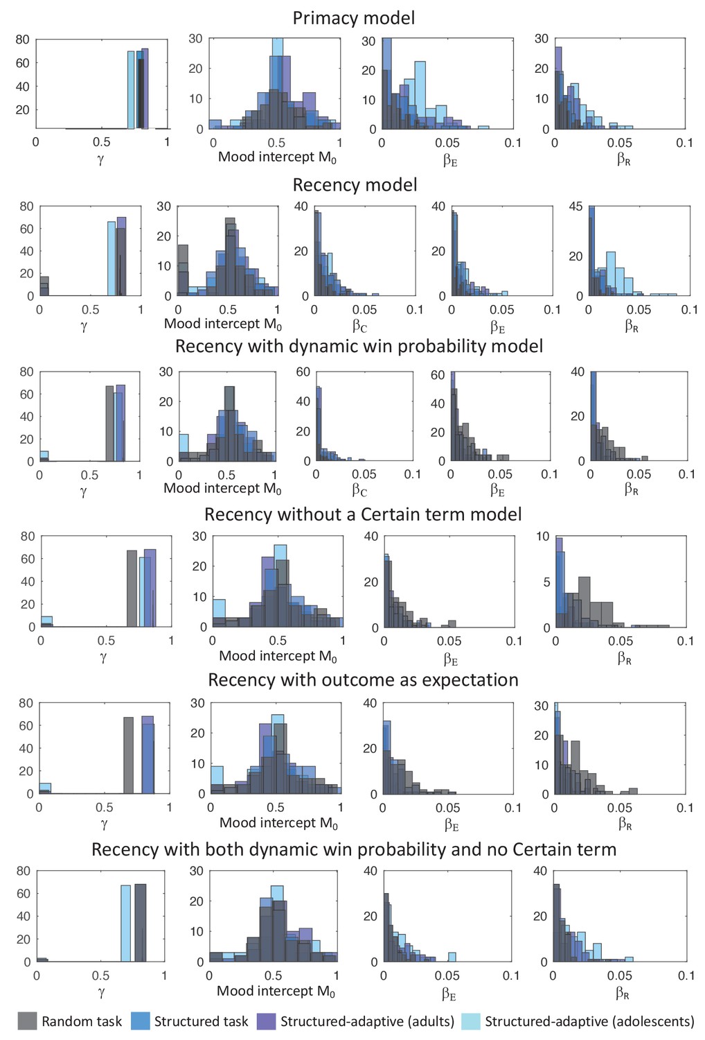
Distributions of the estimated coefficients for the parameters of the Primacy and the different Recency models.
Figure 3—figure supplement 2
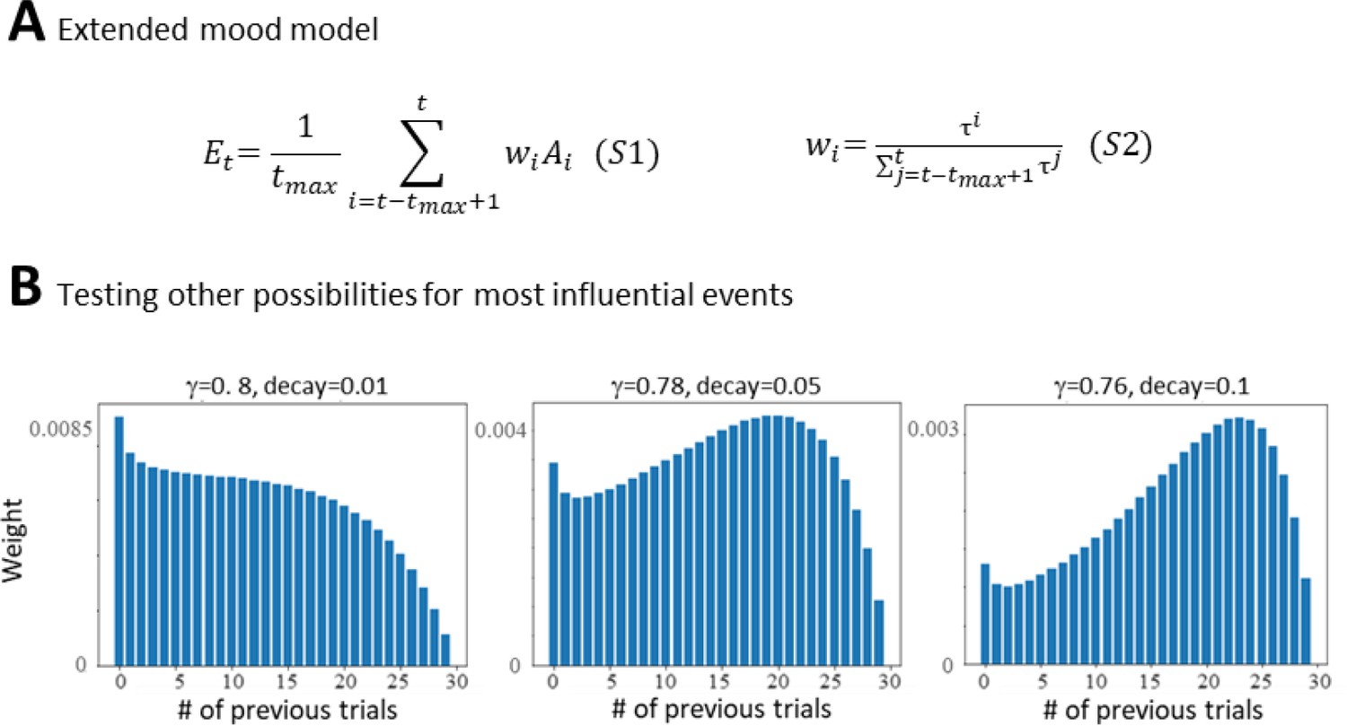
Expanding the Primacy model.
(A) Equations S1 and S2 show the two additional parameters that were included in the Primacy model to test other scaling curves for most influential events on mood. (B) Examples of theoretical scaling curves that were tested with the extended model that were also outperformed by the Primacy model.
Figure 3—figure supplement 3

Mood ratings and the respective trial-wise model parameters.
The left two columns show the task mood ratings and outcomes (A) above the expectation and reward prediction error (RPE) parameters of the Primacy (B) and the Recency (C) models (of a single participant during the Structured task). The rightmost column shows the average across all participants of mood ratings, above the combination between the expectation and RPE parameters of each model (shaded areas represent standard deviation).
Figure 4 with 2 supplements
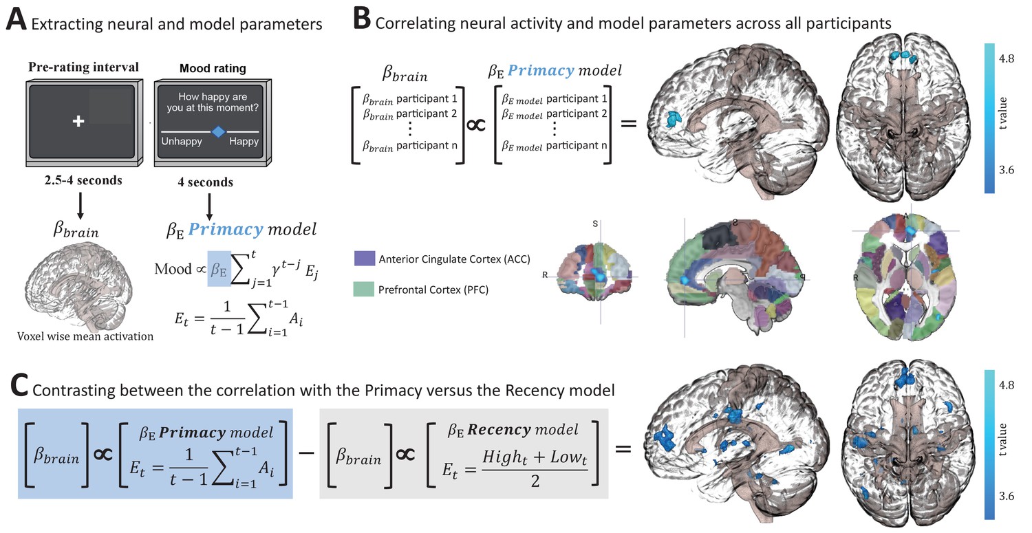
Neural correlates of the Primacy model.
(A) Extracting individual whole-brain BOLD signal activation maps () during the time interval preceding each mood rating, and individual model parameters by fitting mood ratings with the Primacy model (). (B) Correlation across participants between the individual weights of the model expectation term, , and the individual voxel-wise neural activations. A significant cluster was received with a peak at [–3,52,6], size of 132 voxels, threshold at p = 0.0017 (after a multiple comparisons correction as well as a Bonferroni correction for the three 3dMVM models we tested). Below, the resulting cluster of significant correlation is presented aligned on the Automated Anatomical Labeling (AAL) brain atlas for spatial orientation (focus point of the image is at [–7.17,50,4.19], which is located in the ACC region). (C) A statistical comparison between the relation of brain activation to the Primacy versus the Recency models. We compared the regression coefficients of the correlation between participants’ brain activation and the Primacy expectation term weights versus the regression coefficients of the relation to the Recency model expectation term (see Figure 4—figure supplement 1 for the two images before thresholding and before contrasting against each other). This contrast showed a significantly stronger relation of the Primacy model expectation weight to brain signals at [–11,49,9], extending to a cluster of 529 voxels (p = 0.0017). See Materials and methods for a link to the online repository from where the neural analyses scripts and the presented images can be downloaded.
Figure 4—figure supplement 1
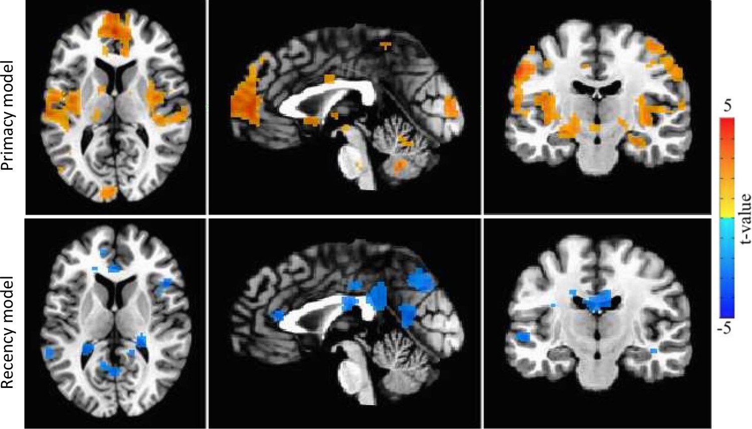
Uncorrected raw data neural correlates of the Primacy model and two Recency models, the original one and the one with the most similar characteristics to the Primacy model (with both dynamic win probability and elimination of the Certain term).
None of the Recency models’ clusters survived correction. Images show correlation across participants between the individual weights of the model expectation term, βE, and the individual whole-brain BOLD signal activation during the time interval preceding each mood rating (an uncorrected threshold of p = 0.05 and a minimal cluster size of 50 voxels).
Figure 4—figure supplement 2
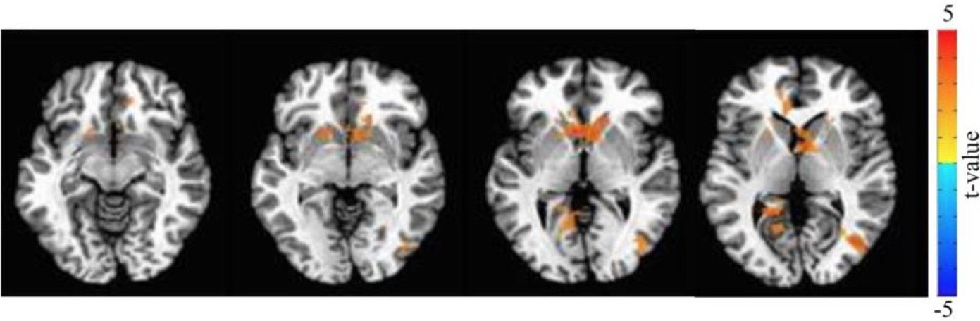
Mood encoding at the whole-brain level in the structured-adaptive task: mood encoding values are derived using the mood ratings as the parametric linear modulator of the BOLD signals during the pre-rating interval (at this interval, which lasts between 2.5 and 4 s, participants are presented with the mood question, but cannot rate their mood yet).
Cluster peaks in the nucleus accumbens (NACC) and covers the ACC and Caudate (337 voxels, t = 4.96).
Tables
Table 1
Performance of the Primacy model versus alternative Recency models in three different reward environments (in adults) and in a lab-based sample comprising adolescent participants, of which 40% were diagnosed as clinically depressed (using the structured-adaptive task).
Statistical comparison is of the streaming prediction errors. (MSE: mean squared error; IQR: interquartile range).
| Model | MSE median | IQR | z-Value | p-Value | ||
|---|---|---|---|---|---|---|
| Reward environment | Random task | Primacy | 0.0165 | 0.0099 | - | - |
| Recency | 0.0171 | 0.0091 | 1.8480 | 0.0323 | ||
| Recency with dynamic win probability | 0.0170 | 0.0078 | 2.7440 | 0.0030 | ||
| Recency without a Certain term | 0.0176 | 0.0099 | 1.9973 | 0.0229 | ||
| Recency with outcome as expectation | 0.0187 | 0.0114 | 3.0053 | 0.0013 | ||
| Recency with both dynamic win and no Certain | 0.0171 | 0.0079 | 2.7440 | 0.0030 | ||
| Structured task | Primacy | 0.0088 | 0.0036 | - | - | |
| Recency | 0.0097 | 0.0069 | 1.6613 | 0.0483 | ||
| Recency with dynamic win probability | 0.0090 | 0.0043 | 1.8853 | 0.0297 | ||
| Recency without a Certain term | 0.0109 | 0.0091 | 3.0053 | 0.0013 | ||
| Recency with outcome as expectation | 0.0141 | 0.0044 | 3.8266 | 0.0001 | ||
| Recency with both dynamic win and no Certain | 0.0090 | 0.0044 | 1.8853 | 0.0290 | ||
| Structured adaptive | Primacy | 0.0137 | 0.0041 | - | - | |
| Recency | 0.0160 | 0.0040 | 3.4533 | 0.0003 | ||
| Recency with dynamic win probability | 0.0171 | 0.0040 | 3.7146 | 0.0001 | ||
| Recency without a Certain term | 0.0189 | 0.0060 | 3.5279 | 0.0002 | ||
| Recency with outcome as expectation | 0.0179 | 0.0063 | 3.6773 | 0.0001 | ||
| Recency with both dynamic win and no Certain | 0.0172 | 0.0040 | 3.6770 | 0.0001 | ||
| Age | Adolescents lab-based | Primacy | 0.0066 | 0.0021 | - | - |
| Recency | 0.0077 | 0.0028 | 3.4533 | 0.0003 | ||
| Recency with dynamic win probability | 0.0079 | 0.0026 | 2.8559 | 0.0021 | ||
| Recency without a Certain term | 0.0094 | 0.0029 | 3.9013 | 0.0000 | ||
| Recency with outcome as expectation | 0.0093 | 0.0038 | 3.6773 | 0.0001 | ||
| Recency with both dynamic win and no Certain | 0.0079 | 0.0027 | 2.9306 | 0.0017 | ||
| Diagnosis | Depressed adolescents | Primacy | 0.0043 | 0.0069 | - | - |
| Recency | 0.0072 | 0.0053 | 3.2666 | 0.0005 | ||
| Recency with dynamic win probability | 0.0075 | 0.0042 | 3.3039 | 0.0004 | ||
| Recency without a Certain term | 0.0074 | 0.0042 | 3.3786 | 0.0003 | ||
| Recency with outcome as expectation | 0.0089 | 0.0043 | 3.9013 | 0.0000 | ||
| Recency with both dynamic win and no Certain | 0.0086 | 0.0069 | 3.4159 | 0.0003 |
Table 2
Participants’ demographics for all datasets.
| Random online MTurk sample | Age | ||
|---|---|---|---|
| (n = 67) | Average | 39.81 | |
| SD | 13 | ||
| Sex | |||
| Male | 37 | ||
| Female | 32 | ||
| Structured online MTurk sample | Age | ||
| (n = 89) | Average | 37.55 | |
| SD | 10.46 | ||
| Sex | |||
| Male | 48 | ||
| Female | 41 | ||
| Structured-adaptive online MTurk sample | Age | ||
| (n = 80) | Average | 37.76 | |
| SD | 11.23 | ||
| Sex | |||
| Male | 46 | ||
| Female | 34 | ||
| Structured-adaptive lab-based sample | Age | ||
| (n = 72) | Average | 15.49 | |
| SD | 1.48 | ||
| Sex | |||
| Male | 17 | ||
| Female | 55 | ||
| MFQ score | |||
| Average | 5.81 | ||
| SD | 5.98 | ||
| Diagnosis | |||
| Healthy volunteer | 29 | ||
| MDD | 43 |
Additional files
-
Supplementary file 1
Model parameters recovery analysis: results of fitting the Primacy and Recency models on simulated datasets as well as a statistical comparison between the two models in both the training errors and the streaming prediction errors.
Note that only streaming prediction errors were used for model selection, and we show the training errors for illustrative purposes.
- https://cdn.elifesciences.org/articles/62051/elife-62051-supp1-v3.docx
-
Supplementary file 2
The formulation of alternative variants of the Recency model.
- https://cdn.elifesciences.org/articles/62051/elife-62051-supp2-v3.docx
-
Transparent reporting form
- https://cdn.elifesciences.org/articles/62051/elife-62051-transrepform-v3.pdf
Download links
A two-part list of links to download the article, or parts of the article, in various formats.
Downloads (link to download the article as PDF)
Open citations (links to open the citations from this article in various online reference manager services)
Cite this article (links to download the citations from this article in formats compatible with various reference manager tools)
The temporal representation of experience in subjective mood
eLife 10:e62051.
https://doi.org/10.7554/eLife.62051


