A unique chromatin profile defines adaptive genomic regions in a fungal plant pathogen
- Department of Plant Pathology, Kansas State University, United States
- Laboratory of Phytopathology, Wageningen University & Research, Netherlands
- Theoretical Biology & Bioinformatics Group, Department of Biology, Utrecht University, Netherlands
- University of Cologne, Institute for Plant Sciences, Cluster of Excellence on Plant Sciences (CEPLAS), Germany
Figures
Figure 1 with 3 supplements

DNA methylation is only present at transposable elements, but not at those present in Lineage-Specific (LS) regions.
(A) Violin plot of the distribution of DNA methylation levels quantified as weighted methylation over genes, promoters, and transposable elements (TEs). Cytosine methylation was analyzed in the CG, CHG, and CHH sequence context. Methylation was measured in the wild-type (WT) and heterochromatin protein one knockout strain (Δhp1). (B, C) Whole chromosome plots showing TE and Gene counts (blue and red heatmaps) and wild-type (black lines) and Δhp1 (green line) CG methylation as measured with bisulfite sequencing. Data is computed in 10 kilobase non-overlapping windows. (C) Two previously defined LS regions (Faino et al., 2016) are highlighted by gray windows. (D) Violin plot of weighted cytosine methylation in 10 kb windows broken into core versus LS location (E) Same as D but plots are for the counts of TEs per 10 kb window. (F) Same as in D but methylation levels were computed at individual TE elements. (A,D,E,F) Statistical differences for indicated comparisons were carried out using non-parametric Mann-Whitney U-test and Holm multiple testing correction with associated p-values shown.
-
Figure 1—source data 1
Genome-wide cytosine methylation levels in 10 kb windows in wild-type and Δhp1 Verticillium dahliae.
- https://cdn.elifesciences.org/articles/62208/elife-62208-fig1-data1-v2.txt
Figure 1—figure supplement 1
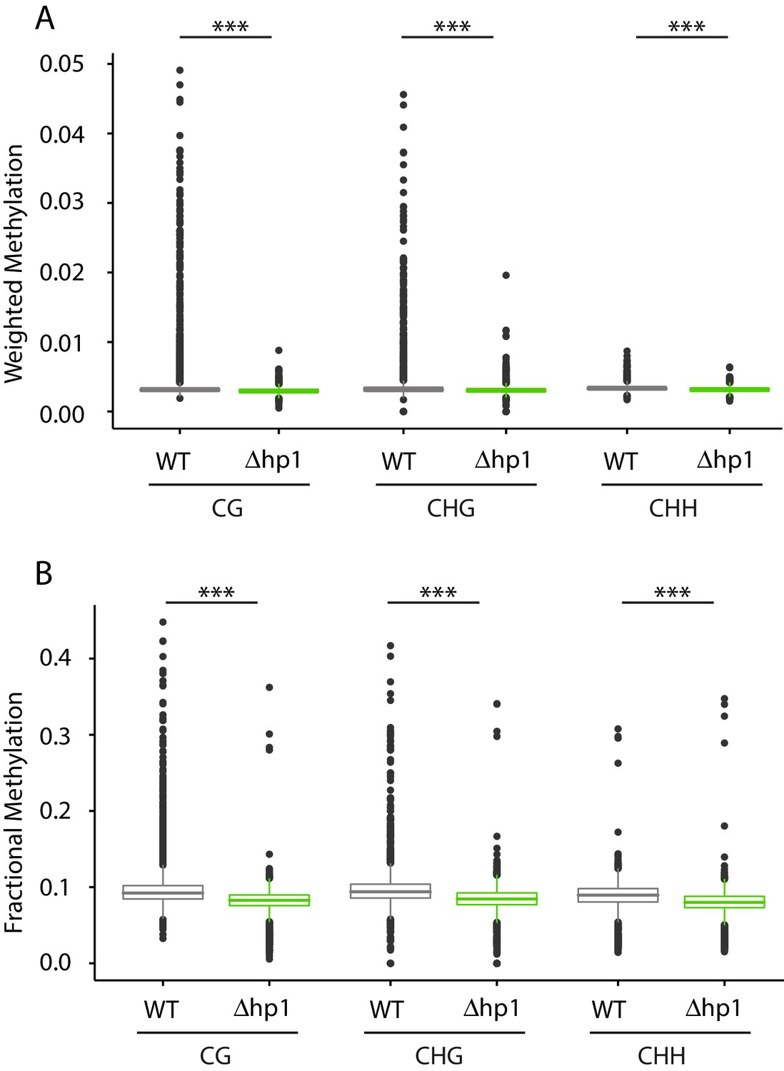
Genome-wide cytosine methylation in wild-type and Dhp1.
(A) Cytosine methylation was calculated using weighted methylation (see Materials and methods) in the CG, CHG, and CHH sequence context in both wild-type (WT) and Dhp1. Methylation levels were determined to be significantly higher in WT using the Mann-Whitney U-test. The symbol (***) indicates p<2.2e-16. (B) Similar to (A), but the genome-wide methylation level was calculated using fractional methylation. All data were summarized in 10 kb bins.
Figure 1—figure supplement 2
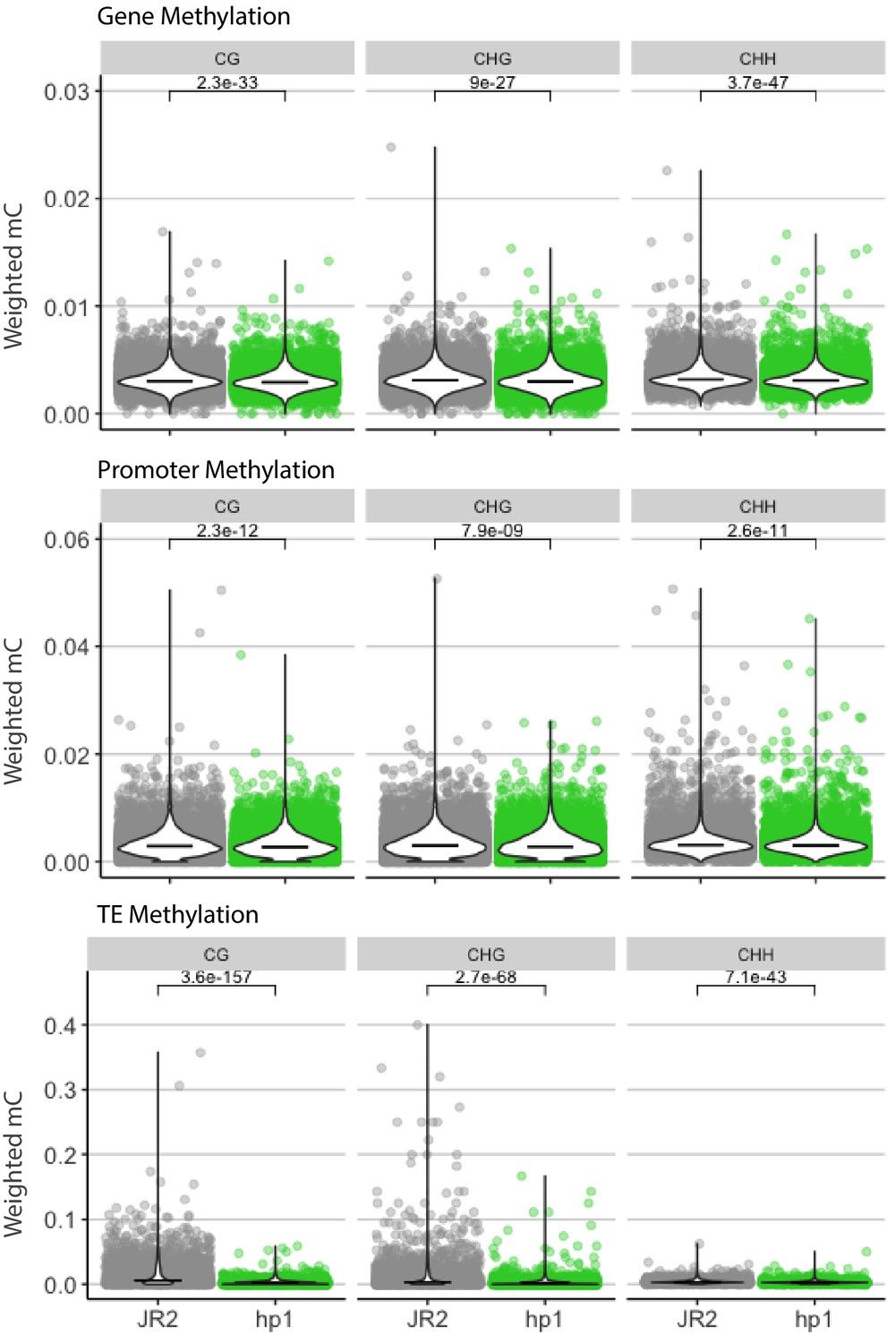
Cytosine methylation for functional elements in wild-type and Dhp1.
Cytosine methylation was calculated using weighted methylation (see Materials and methods) in the CG, CHG, and CHH sequence context in both wild-type (JR2) and Dhp1. DNA methylation was summarized over genes, promoters and TEs as labeled. The individual elements are shown as colored points, along with a violin plot showing the distribution and median as a black line. Methylation levels were determined to be significantly higher in WT, Mann-Whitney U-test with Holm multiple testing correction. Associated p-values are shown.
Figure 1—figure supplement 3
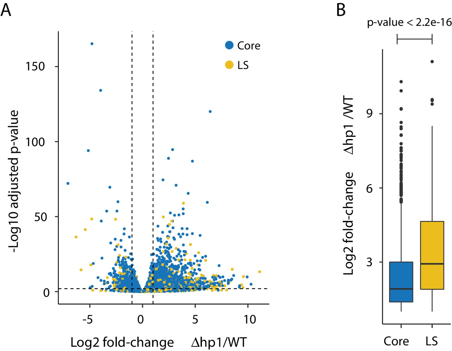
Transcriptional impact of Dhp1.
(A) Volcano plot showing the log2 fold-change for Dhp1 compared to the wild-type (WT) grown in PDB culture. The adjusted p-value (-log10) is shown in the y-axis to indicate statistical significance. Individual genes are shown as colored pointed, with genes in the core (blue) and those in Lineage-Specific (LS; yellow) regions. Genes were considered differentially expressed if they were log2 fold-change < −1 or >1, shown as vertical dashed lines, and an adjusted p-value<0.01, shown as a horizontal dashed line. These cut-offs resulted in 1522 genes more highly expressed in Dhp1, and 587 more highly expressed in wild-type. (B) Bar plot showing the average and range of log2 fold-change values for genes (n = 1522) expressed significantly higher in Dhp1 compared to wild-type from (A). The genes were grouped based on core (blue) versus LS (yellow) location. These groups were statistically significantly different based on Mann-Whitney U-test, p-value<2.2e-16.
Figure 2 with 3 supplements

Individual TE families have distinct epigenetic and physical compaction profiles.
(A) Principle component analysis for 14 variables measured for each individual transposable element (TE). Each vector represents one variable, with the length signifying the importance of the variable in the dimension. The relationship between variables can be determined by the angle connecting two vectors. For angles < 90°, the two variables are correlated, while those >90° are negatively correlated. Each individual element is shown and highlighted by color and symbol as indicated by the key. Colored ellipses show the confidence interval for the four families along with a single large symbol to show the mean position for the four families. mCG, weighted CG DNA methylation; mCHG, weighted CHG DNA methylation; CRI, Composite RIP index; %GC, percent GC sequence content; Identity, Nucleotide identity as percent identity to the consensus TE sequence of a family; Length, element length; Jukes Cantor, Jukes Cantor corrected distance as proxy of TE age; RNAseq, RNA-sequencing reads from (PDB), half strength MS (HMS) or tomato xylem sap (Xylem) grown fungus expressed as variance stabilizing transformed log2 values (see Materials and methods for details); H3K9me3, log2 (TPM+1) values of mapped reads from H3K9me3 ChIP-seq; H3K27me3, log2 (TPM+1) values of mapped reads from H3K27me3 ChIP-seq; ATAC-seq, log2 (TPM+1) values for mapped reads from Assay for transposase accessible chromatin. (B) Ridge plots showing the distribution of the individual TE families per variable. The median value is shown as a solid black line in each ridge. Variables same as in A except for mCG, log2(weighted cytosine DNA methylation + 0.01). (C) Scatter plot for %GC versus CRI values for individual TE elements shown as points. The two plots are for TEs characterized as Unspecified (Unsp) or LTR, labeled in the upper left corner. Each point is colored according to log2 (TPM+1) values from H3K9me3 ChIP-seq, scale shown above each plot. A density plot is shown for both variables on the opposite side from the labeled axis. (D) Same as in C, but the y-axis is now showing the log2 (TPM+1) values from ATAC-seq.
-
Figure 2—source data 1
Genomic data for transposable elements.
- https://cdn.elifesciences.org/articles/62208/elife-62208-fig2-data1-v2.txt
Figure 2—figure supplement 1
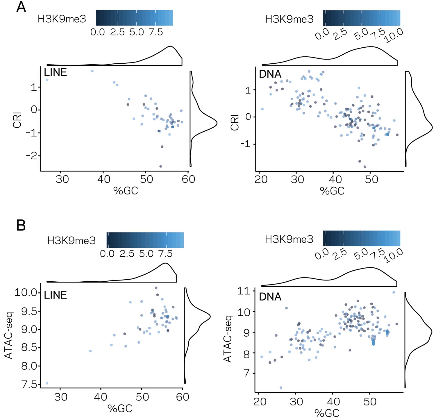
Genomic distribution of DNA characteristics by transposable element (TE) classes.
(A) Scatter plot for %GC sequence content versus CRI values for individual TE elements shown as points, separated by TE type, LINE, and DNA, labeled in the top left of each plot. Each point is colored according to TPM values from H3K9me3 ChIP-seq, scale shown above each plot. A density plot is shown opposite to each respective labeled axis. (B) Similar to (A), but the y-axis is showing the log2 TPM values from ATAC-seq. %GC, The percent GC sequence content; CRI, Composite RIP index; ATAC-seq, Log2 of (TPM+1) values of mapped reads from Assay for Transposase Accessible Chromatin.
Figure 2—figure supplement 2
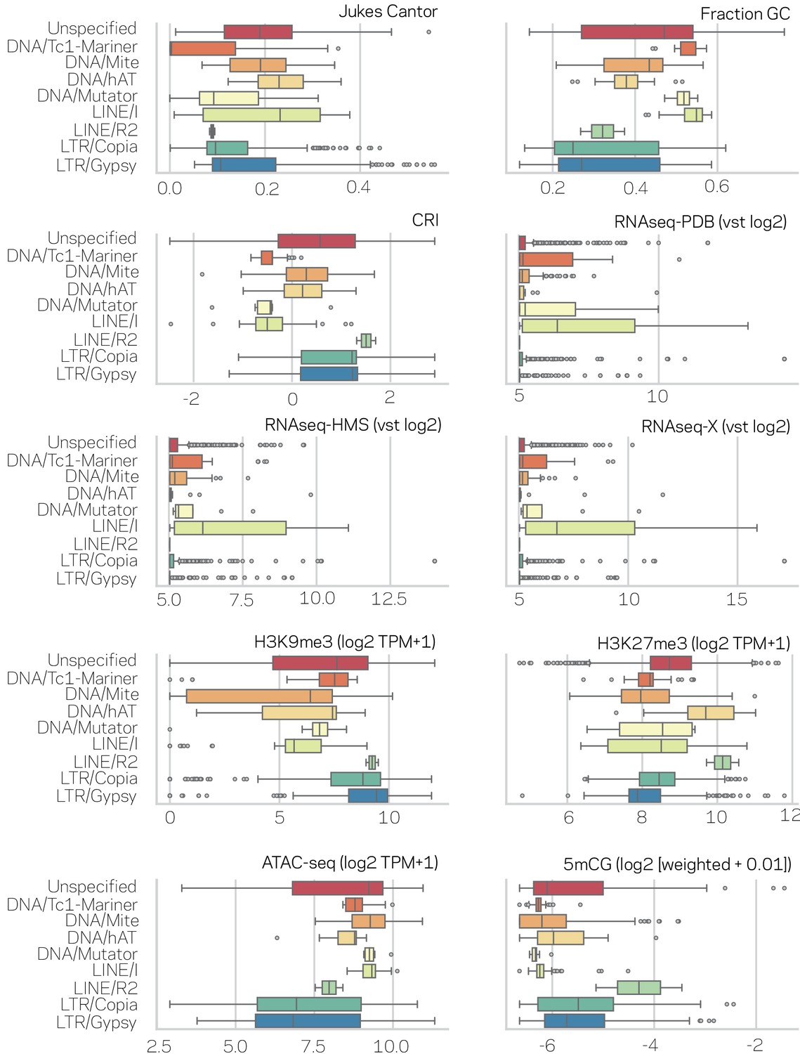
Characterization of transposable elements (TEs) in nine subclasses across genomic variables.
Each data type is shown in the upper right corner of the individual box plots. Outliers are shown as individual points. The nine subclasses of TEs are listed to the left of each figure. Test for significant differences between means of the nine subclasses per data type are shown in Supplementary file 1- table 4 (Kruskal-Wallis test) and significance of individual pair-wise differences are shown in Supplementary file 1- table 5 (Conover test and BH correction).
Figure 2—figure supplement 3
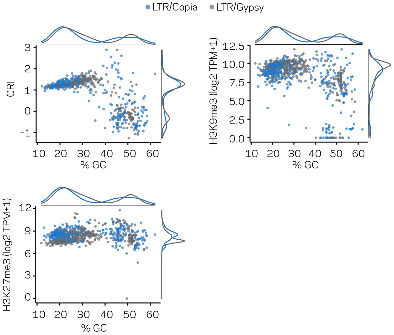
The LTR subclass distinction does not account for the bimodal distribution of LTR elements in the genome.
The same transposable elements (TEs) are shown in three separate scatter plots with marginal densities. Individual Copia elements are shown as blue points, and Gypsy elements as gray points. These plots are related to those shown in Figure 2, but only for the LTR elements. All plots show the % GC variable in the x-axis and different y-axis variables for reference. Clustered patterns of points are not simply accounted for by the two subclasses of LTR elements.
Figure 3 with 1 supplement

The LTR and Unspecified elements have significantly different chromatin profiles based on core versus LS location.
(A) Heatmap comparing core versus LS values within the four TE classifications for the variable listed to the right. Plot colored based on p-values from Wilcoxon rank sum test. p-values≥0.05 are colored white going to red for p-value ≅ 0. (B) Scatter and density plots similar to those shown in Figure 2c except the individual TE points are colored by core (gray) versus LS (red) location. The density plots are also constructed based on the two groupings (C) Similar to B, with the y-axis now showing the log2 (TPM+1) values from ATAC-seq (D) Multiple grouped heatmaps for ten variables collected for each TE. Each row represents a single element and the same ordering is used across all plots. The LS elements are grouped at the top, indicated by the red bar at the top left, and the core elements are grouped below, indicated by the gray bar at the left. Elements are further grouped by the four classifications indicated by the color code shown to the left. Within each element group, the elements are ordered by descending GC content. The scale for each heatmap is shown at the right. GC content, fraction of GC in sequence; Jukes Cantor, corrected distance as proxy of TE age; CRI, Composite RIP index; Length, element length; mCG and mCHG, log2(weighted cytosine DNA methylation+0.01) for CG and CHG, respectively; RNAseq-PDB, variance stabilizing transformed log2 RNA-sequencing reads from PDB grown fungus; H3K9me3 and H3K27me3 and ATAC-seq, TPM values of mapped reads H3K9me3 ChIP-seq, H3K27me3 ChIP-seq, or Assay for transposase accessible chromatin, respectively. Black boxes highlight LTR and Unsp elements in the core that have euchromatin profiles.
Figure 3—figure supplement 1
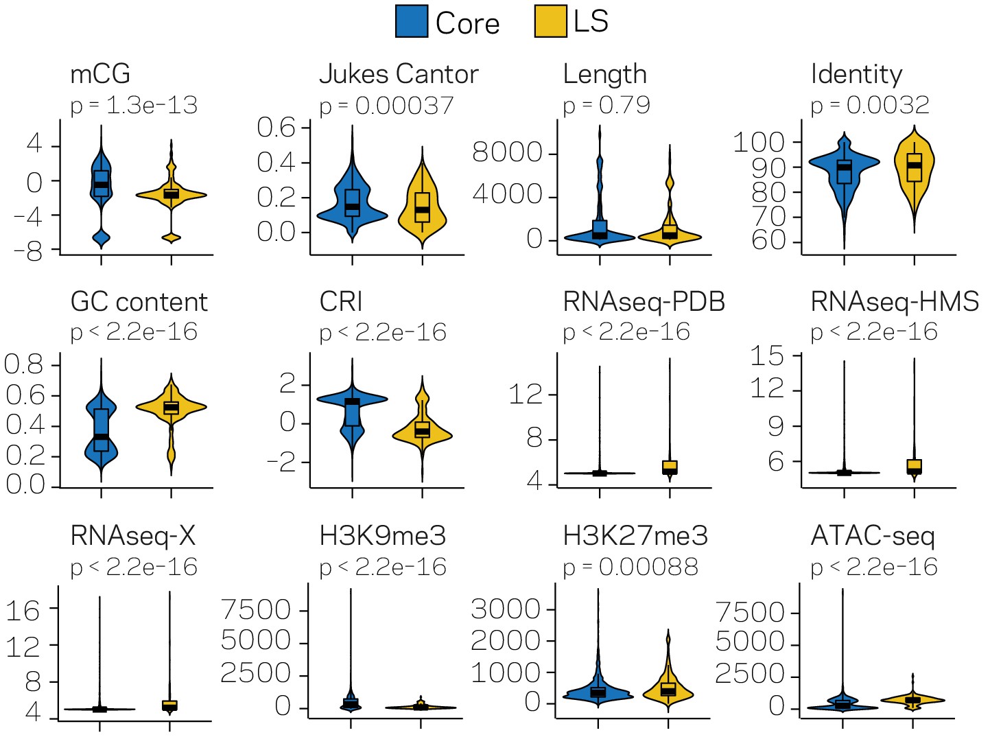
Violin plots for twelve measured variables collected for the TEs located in either the core (blue) or LS (yellow) regions of the genome.
Violin plots show the distribution of the values for each category, along with a box plot showing the mean (thick black line) 1st and 3rd quartiles, and whiskers extending to the furthest data point within 1.5 of the interquartile range. Differences between the core and LS values were measured using the non-parametric Mann-Whitney test and p-values adjusted using the Holm method. Adjusted p-values are shown above each plot. mCG- Log2 weighted cytosine DNA methylation for CG; Jukes Cantor- estimate of sequence divergence from a consensus element; Length- element length in base pairs; Identity- The percent identity of the elements to a family consensus; GC content- The fraction of GC sequence content; CRI- Composite RIP index; RNAseq- variance stabilizing transformed log2 RNA-sequencing reads from Potato Dextrose Broth (PDB), half-Murashige and Skoog (HMS) or Tomato Xylem (X) grown fungi; H3K9me3 and H3K27me3 - TPM values of mapped reads from ChIP sequencing using anti-bodies against the respective histone modifications; ATAC-seq - TPM values of mapped reads from Assay for Transposase Accessible Chromatin.
Figure 4 with 1 supplement
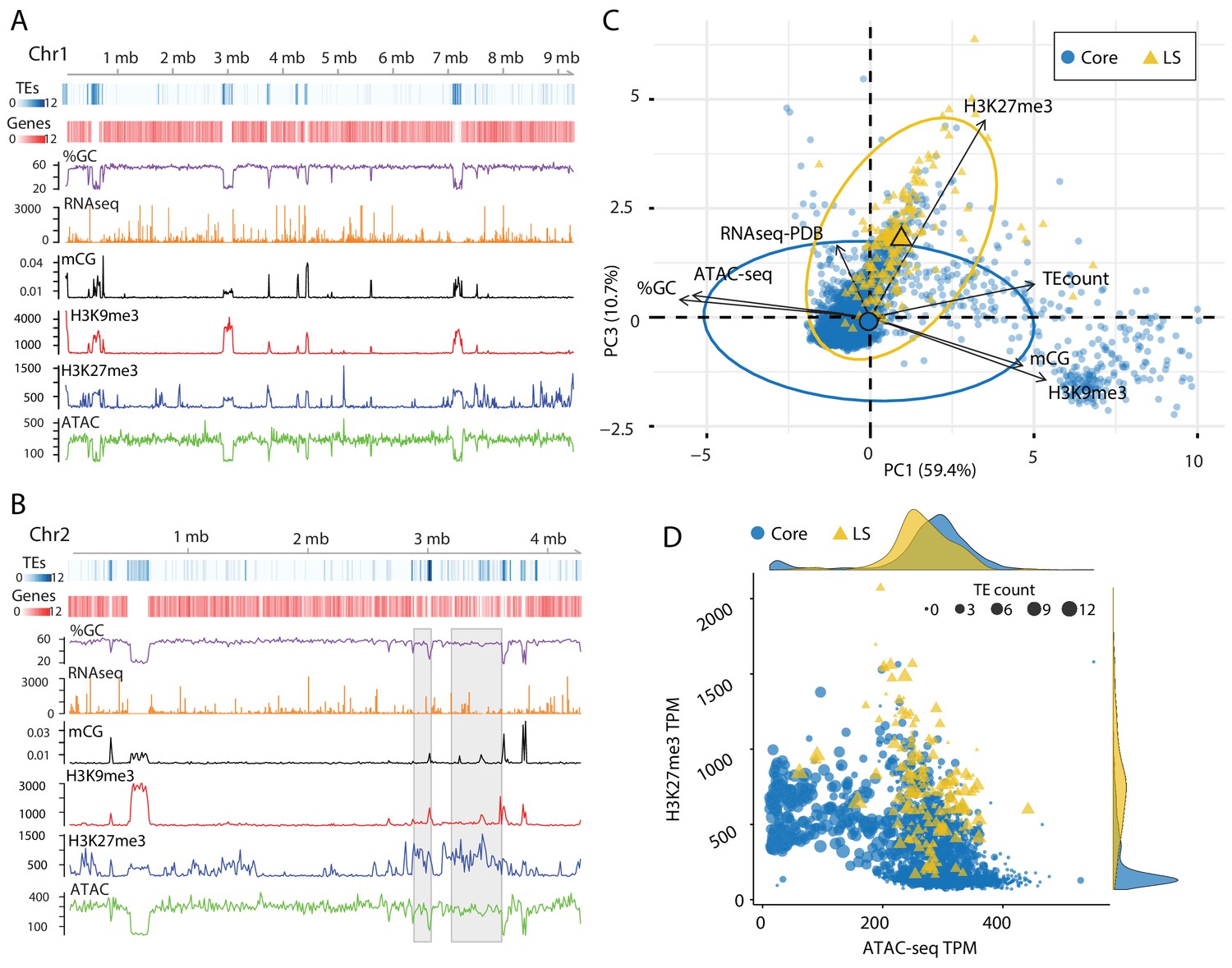
Epigenome and physical DNA characteristics collectively define core and LS regions.
(A and B) Whole chromosomes plots showing TE and gene counts over 10 kb genomic windows, blue and red heatmaps respectively. The %GC content is shown in purple, RNA-seq show in orange, CG cytosine DNA methylation shown in black, H3K9me3 and H3K27me3 ChIP-seq shown in red and blue respectively, and ATAC-seq shown in green. Values are those previously described. (B) Two LS regions are highlighted with a gray window. (C) Principle component analysis for seven variables at each 10 kb window. Dimensions 1 and 3 are plotted and collective explain ~70% of the variation in the data. The individual symbols are colored by genomic location with core (blue circles) and LS (yellow triangles). Colored ellipses show the confidence interval for the core and LS elements with a single large symbol to show the mean. (D) Scatter plot of the 10 kb windows colored for core and LS location by ATAC-seq data (TPM, x-axis) and H3K27me3 (TPM, y-axis). The size of each symbol is proportional to the TE count, shown as five possible ranges from 0 (smallest), 1–3 (next, larger), up to 10–12 (largest). The density plot of each variable is shown on the opposite axis.
-
Figure 4—source data 1
Genomic data for 10 kb windows.
- https://cdn.elifesciences.org/articles/62208/elife-62208-fig4-data1-v2.txt
Figure 4—figure supplement 1

Principle component analysis for seven variables genome wide at 10 kb window.
Each genomic window is shown as a point on the graph, with the windows in the core colored as blue circles and LS as yellow triangles. Colored ellipses show the confidence interval for the core and LS elements with a single large symbol to show the mean. The amount of variation for the first and second dimensions are shown in parentheses. mCG- Log2 weighted cytosine DNA methylation for CG; %GC - The percent GC sequence content; RNAseq-PDB- TPM for RNA-sequencing reads from Potato Dextrose Broth (PDB); H3K9me3 and H3K27me3 - TPM values of mapped reads from ChIP sequencing using anti-bodies against the respective histone modifications; ATAC-seq - TPM values of mapped reads from Assay for Transposase Accessible Chromatin.
Figure 5 with 1 supplement
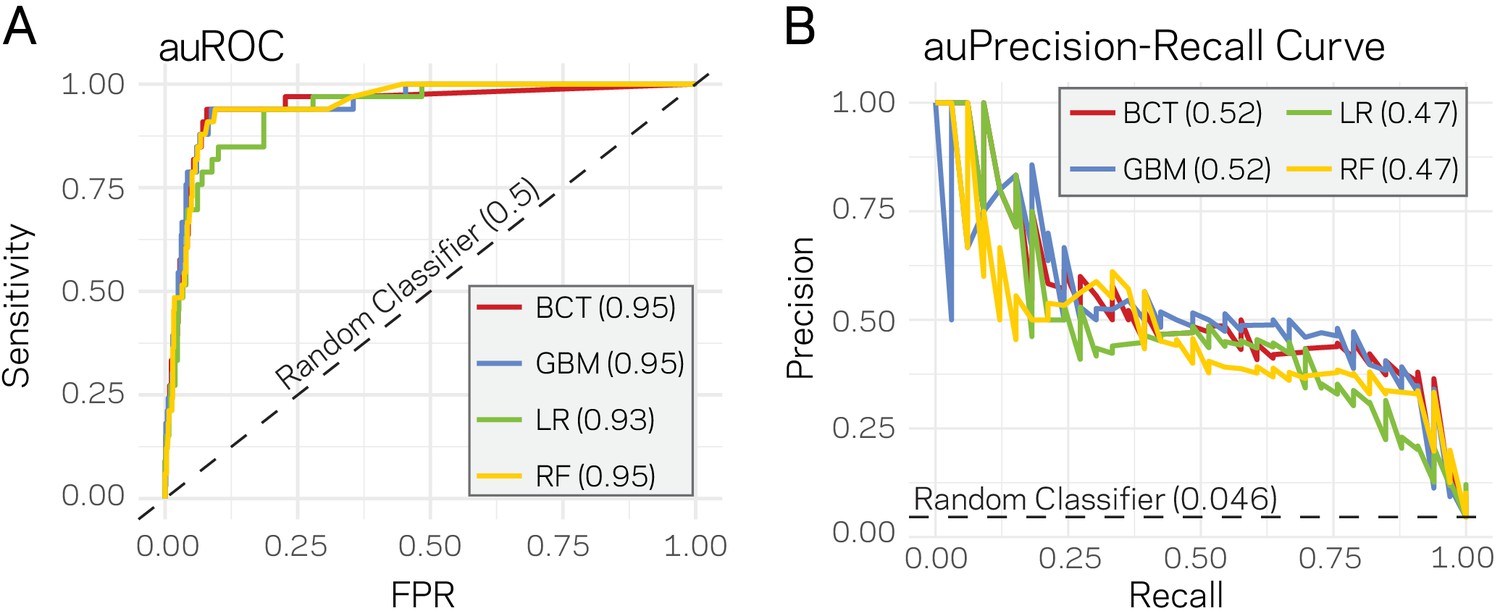
Supervised machine learning can predict Lineage-Specific (LS) regions based on epigenome and physical genome characteristics.
(A) Area under the Response operator curve (auROC) plotting sensitivity and false positive rate (FPR) for four machine learning algorithms, BCT- Boosted classification tree; GBM- stochastic gradient boosting; LR- logistic regression; RF- random forest. The auROC scores are shown next the algorithm key in the gray box. The black dotted line represents the performance of a random classifier. Perfect model performance would be a curve through point (0,1) in the upper left corner. (B) Area under the Precision-Recall curve for the same four models shown in A. Area under the curves are shown in the figure key in the gray box. The black dashed line shows the performance of a random classifier, calculated as the TP / (TP + FN). Perfect model performance would be a curve through point (1,1) in the upper right corner.
Figure 5—figure supplement 1
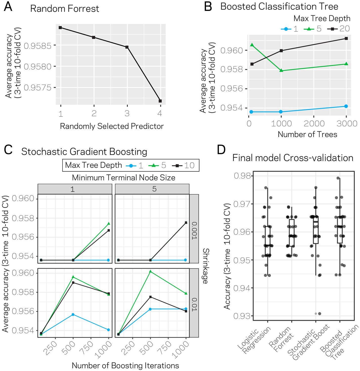
Results from model parameter tuning and assessment.
(A) The random forrest model was trained using three-time 10-fold cross-validation (CV) under varying conditions for the parameter ‘randomly selected predictor’. The plot shows the average accuracy across the 30 trials for each variable level as a black square. (B) Average accuracy results from three-time 10-fold CV using the boosted classification tree algorithm. The variables ‘number of trees’ (x-axis) and ‘max tree depth’ (blue, green, black lines) were varied across the trials. Each data point represents the average accuracy across the CV. (C) Average accuracy results from three-time 10-fold CV using the stochastic gradient boosting algorithm. The variables ‘number of boosting iterations’ (x-axis), ‘shrinkage’ (y-axis), ‘minimum terminal node size’ (columns), and max tree depth (blue, green, black lines) were varied across the trials. Each data point represents the average accuracy across the CV. (D) The individual accuracy measurements and box plot for the final models picked for each algorithm. Results are from the 30 CV runs.
Figure 6 with 5 supplements
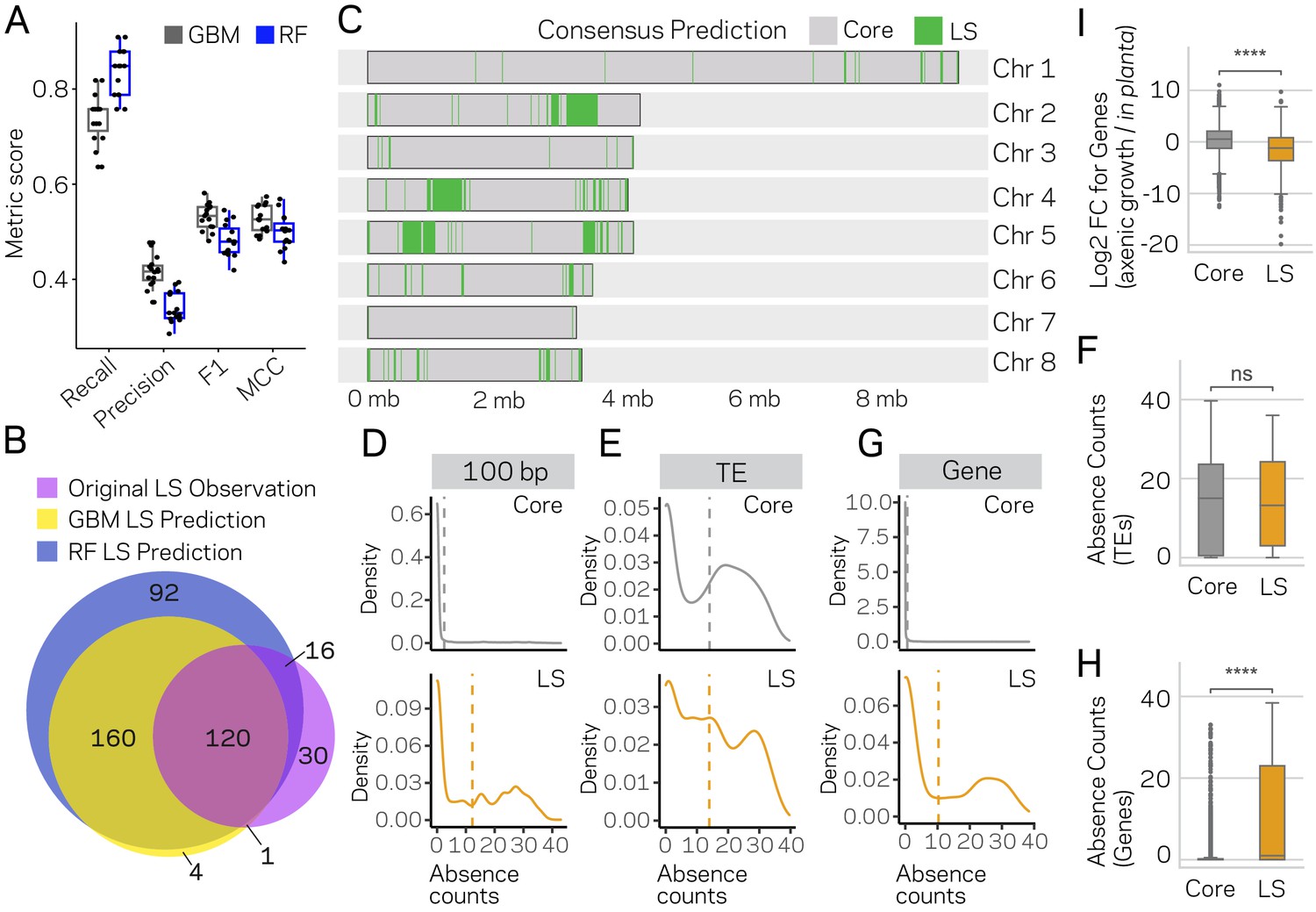
Machine learning predictions for genome-wide LS content.
(A) Two machine learning algorithms, Stochastic Gradient Boosting (GBM) and Random Forest (RF), were used to predict Lineage-Specific (LS) regions from 15 independent training-test splits (80/20). Classifier performance was measured for each of the 15 trials, and summarized as a boxplot with each trial represented as a point. (B) Venn diagram showing the overlap between the results of the two classifiers and the original observations of LS regions (de Jonge et al., 2013; Faino et al., 2016). Each slice of the diagram shows the number of LS regions predicted, see Materials and methods for additional details. (C) Schematic representation of the eight chromosomes (labeled on right) of V. dahliae strain JR2. Core (gray) and LS (green) classification for 10 kb windows. The consensus predictions were those made by both the GBM and RF model (in total 280). (D) Boxplot showing a significant difference for in planta gene induction between core and LS genes, Mann-Whitney U test p-value=1.34e-50. (E) Density distribution for core (gray) and LS (orange) elements based on absence counts over 100 bp windows. The mean absence counts are shown as a dashed vertical line. (F) Similar to E but the analysis was conducted for TEs. (G) Boxplot showing no significant difference between core and LS TE elements for absence counts, Mann-Whitney U test p-value=0.92. (H) Similar to E but the analysis was conducted for genes. (I) Boxplot showing a significant difference between core and LS genes for absence counts, Mann-Whitney U test p-value=3.82e-104. ns, non-significant; **** p-value<1.00e-4.
-
Figure 6—source data 1
Consensus LS classification genomic regions.
- https://cdn.elifesciences.org/articles/62208/elife-62208-fig6-data1-v2.txt
-
Figure 6—source data 2
Gene presence and absence counts.
- https://cdn.elifesciences.org/articles/62208/elife-62208-fig6-data2-v2.update.txt
-
Figure 6—source data 3
TE presence and absence counts.
- https://cdn.elifesciences.org/articles/62208/elife-62208-fig6-data3-v2.update.txt
Figure 6—figure supplement 1
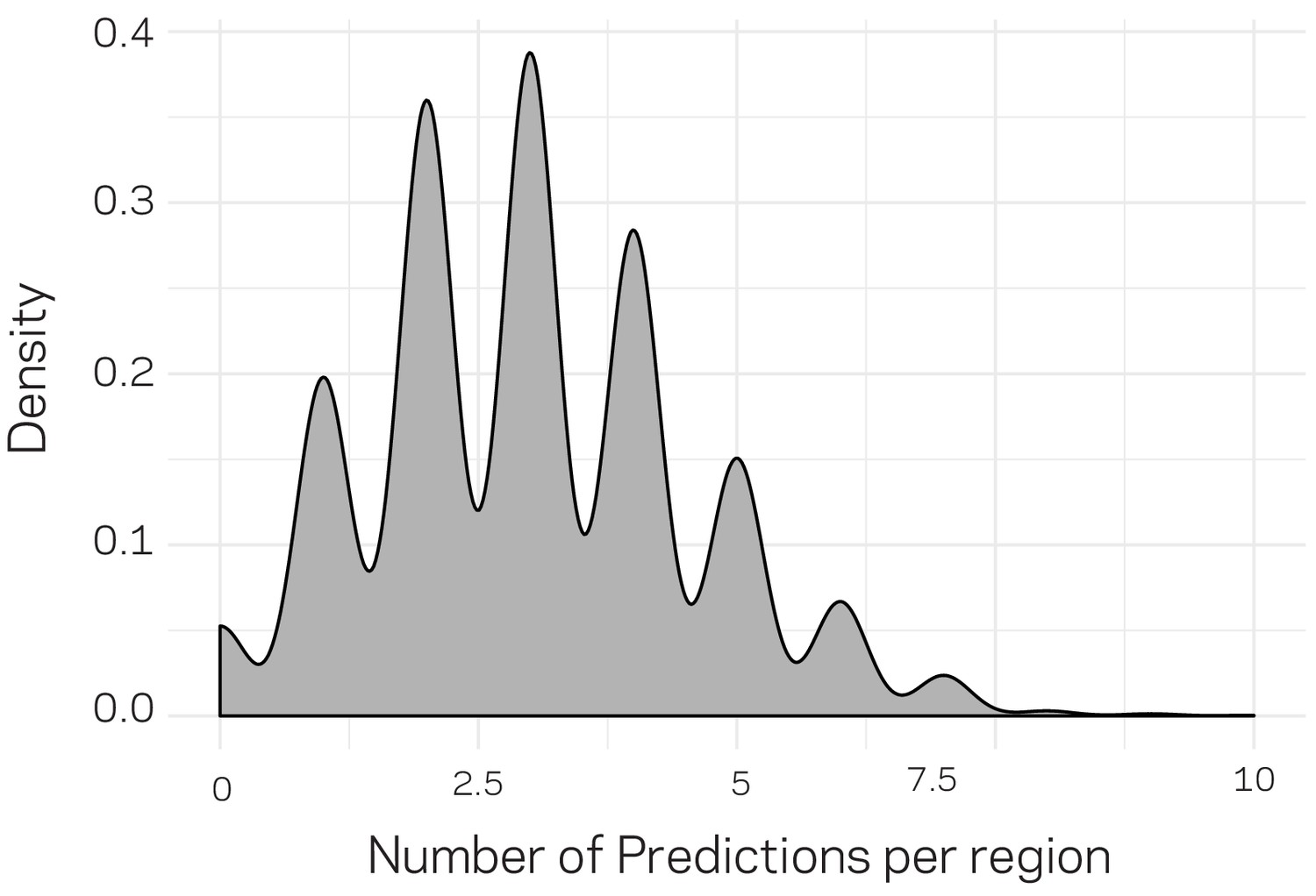
Density plot for the number of distribution of predictions per genomic region.
The genomic data were compiled into 3611 10 kb windows. For machine learning training and testing (related to Figure 6), only 20% of the data could be used for prediction. To generate predictions genome wide, we randomly and independently split the data into training and testing (80:20) an generated predictions. Therefore, each regions could have received more than one prediction. The above distribution profile shows that a majority of the regions received three predictions, with a large proportion of the data having received between 2 and 4 predictions. Only 124 regions received no prediction by change. For each split, we ensured that the population distribution of ~20:1 (core:LS) was maintained in the training and testing data.
Figure 6—figure supplement 2
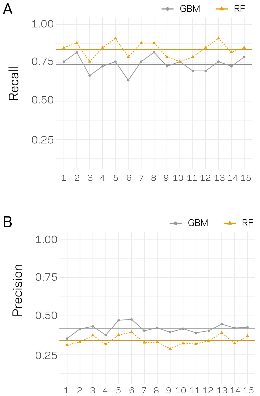
Recall and Precision assessment for independent classification trials.
For each trail, the data set were split 80:20, training and testing, 15 independent times. For each data split, the model was trained and tested and the performance was assessed using Recall (A) and Precision (B). The x-axis’ show the data split trial. Results for each trial are shown as an orange triangle connected with a dashed line for Random Forrest (RF) based classification and a gray point for Stochastic Gradient Boosting (GBM). The mean across the 15 trials is shown by a solid horizontal line of the respective color.
Figure 6—figure supplement 3
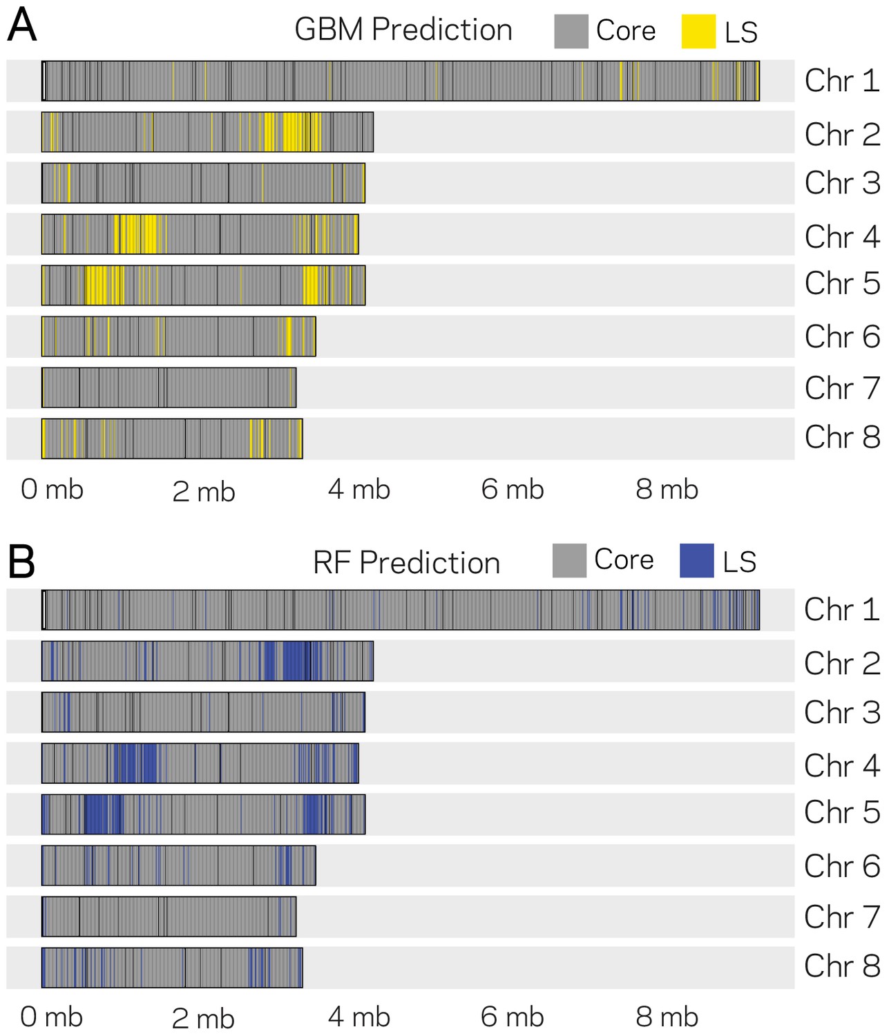
Genomic location of Lineage-Specific (LS) predictions from two ML models.
The eight chromosomes of V. dahliae are labeled at the right (Chr. X) along with the physical DNA size indicated at the bottom. (A) GBM model predictions for 10 kb windows as either core or LS regions are shown in gray and yellow, respectively. The GBM model predicted a total of 285 LS regions. (B) RF model predictions for 10 kb windows as either core and LS regions shown are shown in gray and blue, respectively. The RF model predicted a total of 388 LS regions.
Figure 6—figure supplement 4
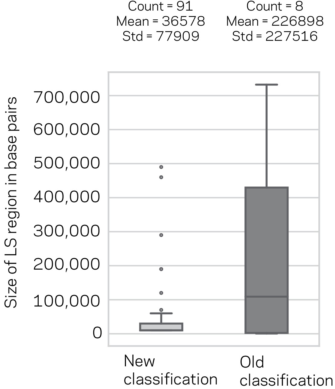
Size distribution and summary description of the New and Old Lineage-Specific (LS) classifications.
Box plot of the LS region sizes for the New classification based on model consensus and the previous LS classification. The number of regions, their mean and standard deviation (Std) are shown above the respective box plots. The means were not statistically significantly different, Mann-Whitney U-Test, p-value=0.93.
Figure 6—figure supplement 5
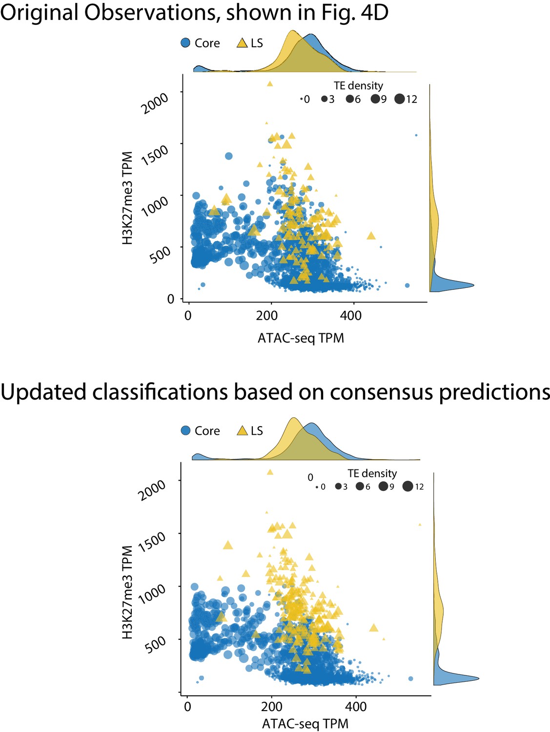
Genome model of core and Lineage-Specific (LS) regions defined by epigenetics and chromatin status.
(Top) The genome of V. dahliae was split into 10 kb windows, and labeled as core or LS based on previous observations, shown in Figure 4D, re-shown here for comparison. (Bottom) Same 10 kb genomic windows and data, but the regions are now defined as core and LS based on the consensus machine learning predictions. The core regions are shown in blue as circles. LS regions shown as yellow triangles. Points are plotted according to TPM ATAC-seq signal (x-axis) and H3K27me3 ChIP-seq TPM (y-axis). The size of each point is proportional to the number of TEs in the 10 kb window, shown as TE density. The marginal density plots are shown opposite of the respective axis.
Figure 7 with 3 supplements
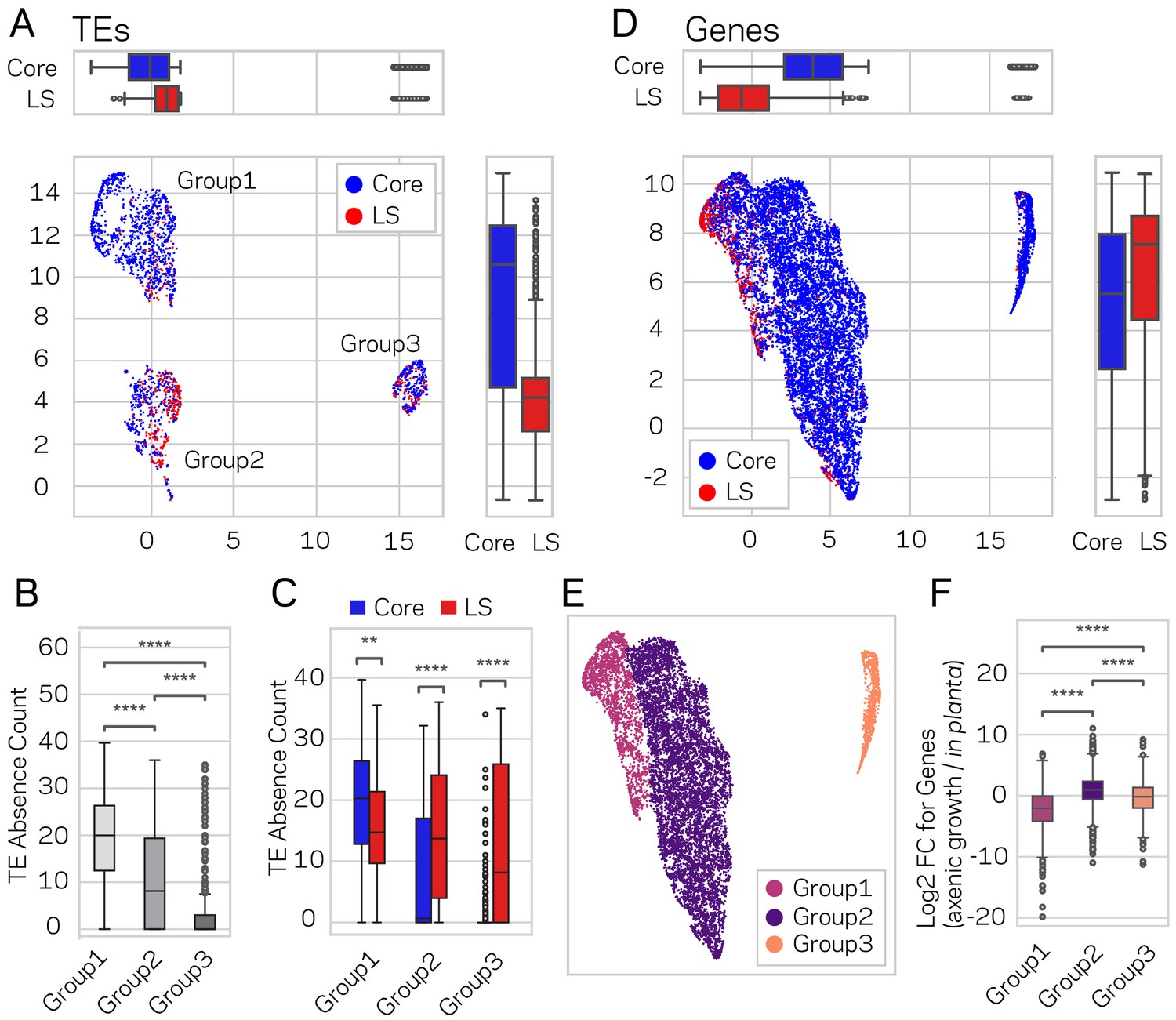
Genome-wide UMAP groups details that functional elements labeled core and LS have different epigenetic and DNA characteristics.
(A) Uniform Manifold Approximation and Projection (UMAP) clustering of individual V. dahliae TEs, color coded for core (blue) and LS (red). UMAP clustering in two dimensions resulted in the identification Group1, 2, and 3 elements. Boxplots are shown opposite of the x- and y-axis to quantify the UMAP designation of the LS and core elements. Statistical difference measured using Mann-Whitney U test for UMAP labeling on the x-axis, p-value=1.77e-38, and y-axis, p-value=9.04e-80. (B) Boxplot for TE absence counts for UMAP Group1, 2, and 3 elements. Statistical difference measured using Conover’s test and Holm multiple-test correction of p-values (C) Boxplot for TE absence counts for LS and core elements in UMAP Group1, 2, and 3. Statistical difference measured using Mann-Whitney U test and Holm multiple-test correction of p-values. (D) Similar UMAP clustering as shown in (A), but performed using genes as the clustering elements shown as individual dots. Marginal boxplots shown as in (A), x-axis p-value=5.45e-221, and y-axis p-value=1.84e-28. (E) UMAP gene clustering, color coded to show three groups. (F) Boxplot for in planta gene induction for UMAP Group1, 2, and 3 genes. Statistical difference measured using Conover’s test and Holm multiple-test correction of p-values. **, p-value<0.01; ****, p-value<0.0001.
-
Figure 7—source data 1
Genomic data and UMAP group for TEs.
- https://cdn.elifesciences.org/articles/62208/elife-62208-fig7-data1-v2.txt
-
Figure 7—source data 2
Genomic data and UMAP group for genes.
- https://cdn.elifesciences.org/articles/62208/elife-62208-fig7-data2-v2.txt
Figure 7—figure supplement 1
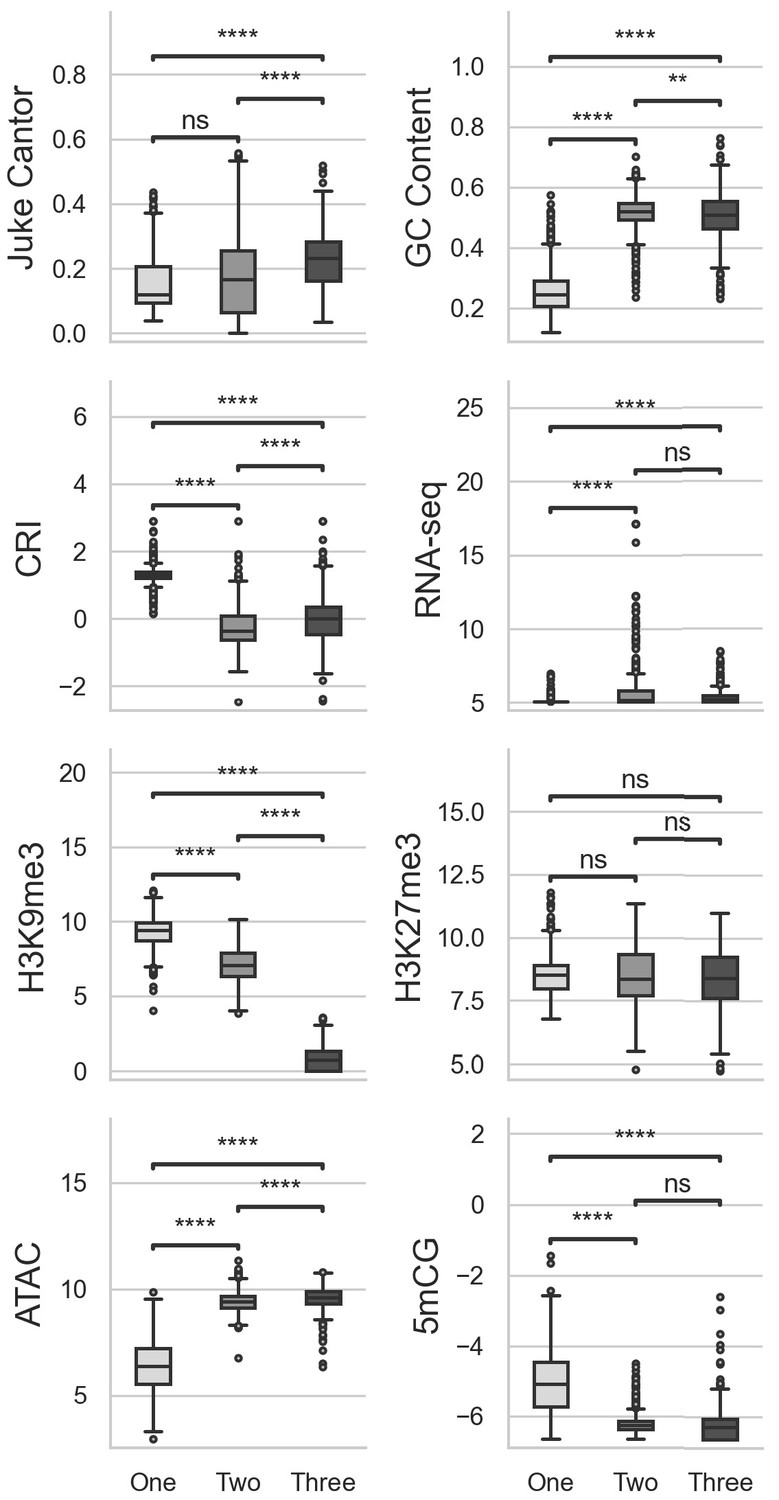
Multiple comparisons of transposable elements (TEs) in UMAP groups for genomic variables.
GC content, GC sequence fraction; Jukes Cantor, corrected Jukes Cantor distance of TE comparisons; CRI, Composite RIP index; RNAseq, variance stabilizing transformed log2 RNA-sequencing reads from Xylem-media grown fungus; H3K9me3 and H3K27me3 and ATAC-seq, TPM values of mapped reads from H3K9me3 ChIP-seq, H3K27me3 ChIP-seq, or Assay for transposase accessible chromatin respectively; 5mCG, log2 weighted cytosine DNA methylation+0.01 for CG. Pairwise comparisons were performed using Conover’s test, with Holm multiple testing correction. **, p-value<0.01; ****, p-value<0.0001.ns, Non-significant p-value at a = 0.05.
Figure 7—figure supplement 2
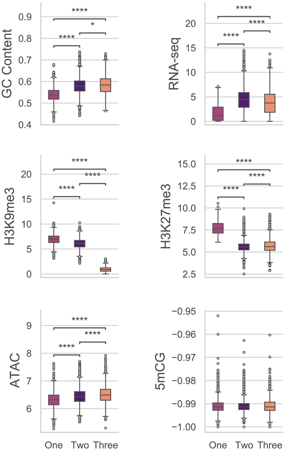
Multiple comparisons of Genes in UMAP groups for genomic variables.
GC content, GC sequence fraction; RNAseq, log2 TPM+1 of RNA-sequencing reads from PDB grown fungus; H3K9me3 and H3K27me3 and ATAC-seq, TPM values of mapped reads from H3K9me3 ChIP-seq, H3K27me3 ChIP-seq, or Assay for transposase accessible chromatin respectively; 5mCG, log2 weighted cytosine DNA methylation+0.01 for CG. There were no significant differences for the comparisons of DNA methylation levels at a = 0.05. Pairwise comparisons were performed using Conover’s test, with Holm multiple testing correction. *, p-value<0.05; ****, p-value<0.0001.
Figure 7—figure supplement 3

UMAP groupings vary significantly for Absence across V.
dahliae strain. (A) Scatter plot showing each 11,429 genes as a point following the UMAP results. Each gene is colored according to its absence count across 42 V. dahliae strains. (B) Box plot showing the distribution of gene absence counts for each of the three UMAP groups. (C) Similar plot as shown in A, but only genes that have an absence count greater than zero are plotted. (D) Similar to B, but only genes that have an absence count greater than zero are plotted. Pairwise comparisons were performed using Conover’s test, with Holm multiple testing correction. There were 2130, 8140, and 1159 genes in UMAP Group1, 2, and 3 respectively for A and B. There were 666, 3156 and 441 genes in UMAP Group1, 2, and 3 respectively for C and D. ns, non-significant a = 0.05; ****, p-value<0.0001.
Tables
Table 1
Summary of DNA methylation in Verticillium dahliae wild-type (WT) and heterochromatin protein one deletion mutant (Δhp1) as measured by whole genome bisulfite sequencing calculated over 10 kb non-overlapping windows.
| Genotype | Avg. weighted mCG* | Avg. weighted mCHG* | Avg. weighted mCHH* | Avg. fraction mCG* | Avg. fraction mCHG* | Avg. fraction mCHH* |
|---|---|---|---|---|---|---|
| WT | 0.0040 | 0.0037 | 0.0034 | 0.097 | 0.097 | 0.088 |
| Δhp1 | 0.0030 | 0.0030 | 0.0032 | 0.082 | 0.083 | 0.079 |
-
Avg. Weighted, The average of total methylated cytosines in a given context divided by total cytosines in that context in a 10 kb windows; Avg. Fraction, The total cytosine positions with a read supporting methylation divided by total cytosines in a specific context in a 10 kb window; mCG, methylated cytosine residing next to a guanine; mCHG, methylated cytosine residing next to any base that is not a guanine next to a guanine; mCHH, methylated cytosine residing next to any two bases that are not a guanines. *, values are significantly different (p-value<0.001), Mann-Whitney U-test. The distribution of values and p-values for individual comparisons are shown in Figure 1—figure supplement 1.
Table 2
Confusion Matrix for LS and core prediction in V.dahliae from test data classification using the final trained model.
| Known | |||
|---|---|---|---|
| Predicted | Core | LS | |
| LR | Core | 638 | 7 |
| LS | 50 | 26 | |
| GBM | Core | 645 | 5 |
| LS | 43 | 28 | |
| BCT | Core | 672 | 20 |
| LS | 16 | 13 | |
| RF | Core | 623 | 2 |
| LS | 65 | 31 | |
-
LR, Logistic Regression; GBM, Stochastic Gradient Boosting; BCT, Boosted Classification Tree; RF, Random Forest; Core, regions of the genome defined as core; LS, regions of the genome defined as Lineage Specific. For final model parameter settings and classification thresholds, see Materials and methods.
Table 3
Assessment of four trained machine learning algorithms on final test data.
| Models | Precision | Recall | MCC | F1 |
|---|---|---|---|---|
| LR | 0.34 | 0.79 | 0.49 | 0.48 |
| GBM | 0.39 | 0.85 | 0.55 | 0.54 |
| BCT | 0.45 | 0.39 | 0.39 | 0.42 |
| RF | 0.32 | 0.94 | 0.52 | 0.48 |
-
LR, Logistic Regression; GBM, Stochastic Gradient Boosting; BCT, Boosted Classification Tree; RF, Random Forest; MCC, Matthews Correlation Coefficient; F1, F-score or harmonic mean of precision and recall. For final model parameter settings and classification thresholds, see Materials and methods.
Key resources table
| Reagent type (species) or resource | Designation | Source or reference | Identifiers | Additional information |
|---|---|---|---|---|
| Strain, strain background (V. dahliae) | JR2, wild-type | PMID:26286689 | Fungal Biodiversity Center (CBS), 143773 | |
| Strain, strain background (V. dahliae) | JR2, Δhp1 | https://doi.org/10.1101/2020.08.26.268789 | ||
| Antibody | Rabbit anti H3K9me3 (Polyclonal) | Active Motif | 39765 | ChIP (1:200) |
| Antibody | Rabbit anti H3K27me3 (Polyclonal) | Active Motif | 39155 | ChIP (1:200) |
| Recombinant DNA reagent | pRF-HU2 | Frandsen et al., 2008 | USER-cloning | |
| Commercial assay or kit | EZ DNA Methylation-Gold kit | Zymo Research | D5005 | |
| Commercial assay or kit | Nextera DNA library Preparation | Illumina | FA-121–1030 |
Additional files
-
Supplementary file 1
Supplementary tables.
Table 1. Summary of Transposable elements by Family in core and LS regions. Table 2. Dunns test of pairwise differences for TE Families following Kruskal-Wallis test. Table 3. Summary count of TEs by sub-class. Table 4. Kruskal-wallis test statistic for differences between TE sub-classes for genomic variables. Table 5. P-value results from Conover test and BH multiple testing correction for genomic variables summarized over TE sub-classes. Table 6. Contribution of variables to the first 5 dimensions of PCA. Table 7. Confusion Matrix results for Stochastic Gradient Boosting machine learning of 15 independent training-test predictions of LS and core regions. Table 8. Confusion Matrix results for Random Forest machine learning of 15 independent training-test predictions of LS and core regions. Table 9. GMB LS prediction results for each of the 15 rounds of training and testing. Table 10. RF LS prediction results for each of the 15 rounds of training and testing. Table 11. Contingency tables for observed and expected LS versus core designation for in planta induction. Table 12. Contingency tables for observed and expected LS versus core designation for predicted effectors. Table 13.Contingency tables for observed and expected LS versus core designation for proteins with secretion signal. Table 14. Contingency tables for observed and expected TE elements classified as LS and core in the 3 UMAP Groups. Table 15. Kruskal-wallis test statistic for differences between TE UMAP groups across genomic variables. Table 16. Contigency tables for observed and expected genes classified as LS and core in the 3 UMAP Groups3. Table 17. Kruskal-wallis test statistic for differences between Gene UMAP groups across genomic variables. Table 18. Verticillium dahliae isolates used for the presence/absence variation.
- https://cdn.elifesciences.org/articles/62208/elife-62208-supp1-v2.xlsx
-
Transparent reporting form
- https://cdn.elifesciences.org/articles/62208/elife-62208-transrepform-v2.docx
Download links
A two-part list of links to download the article, or parts of the article, in various formats.
Downloads (link to download the article as PDF)
Open citations (links to open the citations from this article in various online reference manager services)
Cite this article (links to download the citations from this article in formats compatible with various reference manager tools)
A unique chromatin profile defines adaptive genomic regions in a fungal plant pathogen
eLife 9:e62208.
https://doi.org/10.7554/eLife.62208


