The connectome of the adult Drosophila mushroom body provides insights into function
- Janelia Research Campus, Howard Hughes Medical Institute, United States
- Department of Neuroscience, Columbia University, Zuckerman Institute, United States
- Drosophila Connectomics Group, Department of Zoology, University of Cambridge, United Kingdom
- Centre for Neural Circuits & Behaviour, University of Oxford, United Kingdom
- Neurobiology Division, MRC Laboratory of Molecular Biology, United Kingdom
Figures
Figure 1 with 2 supplements
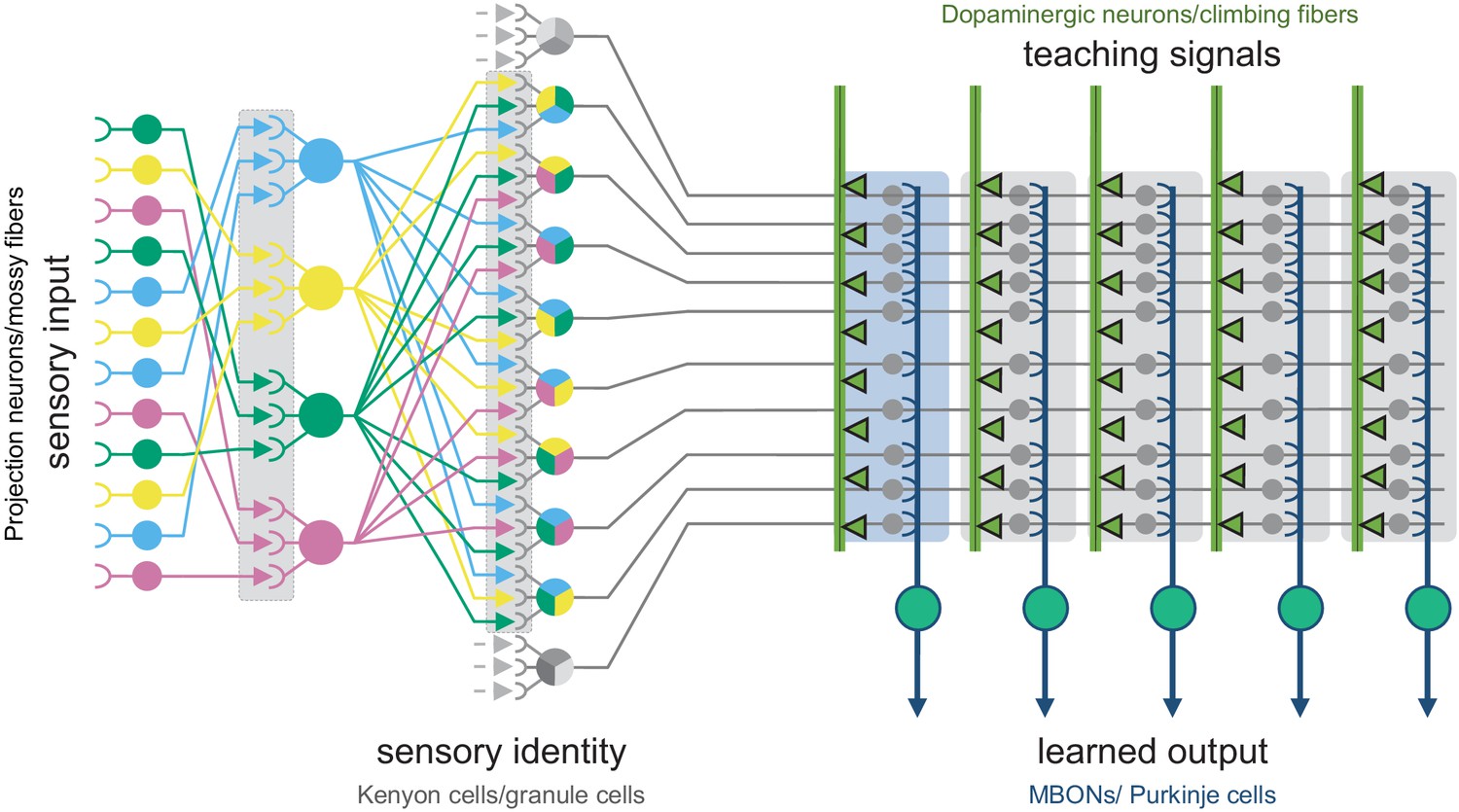
The shared circuit architecture of the mushroom body and the cerebellum.
In both the insect MB and the vertebrate cerebellum sensory information is represented by sparse activity in parallel axonal fibers; Kenyon cells (KCs) in the MB and granule cells (GCs) in the cerebellum (reviewed in Modi et al., 2020). In general, each KC or GC has claw-like dendrites that integrate sensory input from a small number of neurons, called projection neurons in insects and mossy fibers in vertebrates. In the MB, teaching signals are provided by dopaminergic neurons (DANs) and in the cerebellum by climbing fibers. Learned output is conveyed to the rest of the brain from the MB lobes by MB output neurons (MBONs) or, from the cerebellar cortex, by Purkinje cells. The arbors of the DANs and MBONs overlap in the MB lobes and define a series of 15 compartments (Aso et al., 2014a; Gao et al., 2019 ; Figure 2; Figure 1—video 2); similarly, overlap between the arbors of climbing fibers and Purkinje cells define zones along the GC parallel fibers.
Figure 1—video 1
Introduction to the MB.
Figure 1—video 2
Introduction to MB compartments.
Figure 2 with 1 supplement
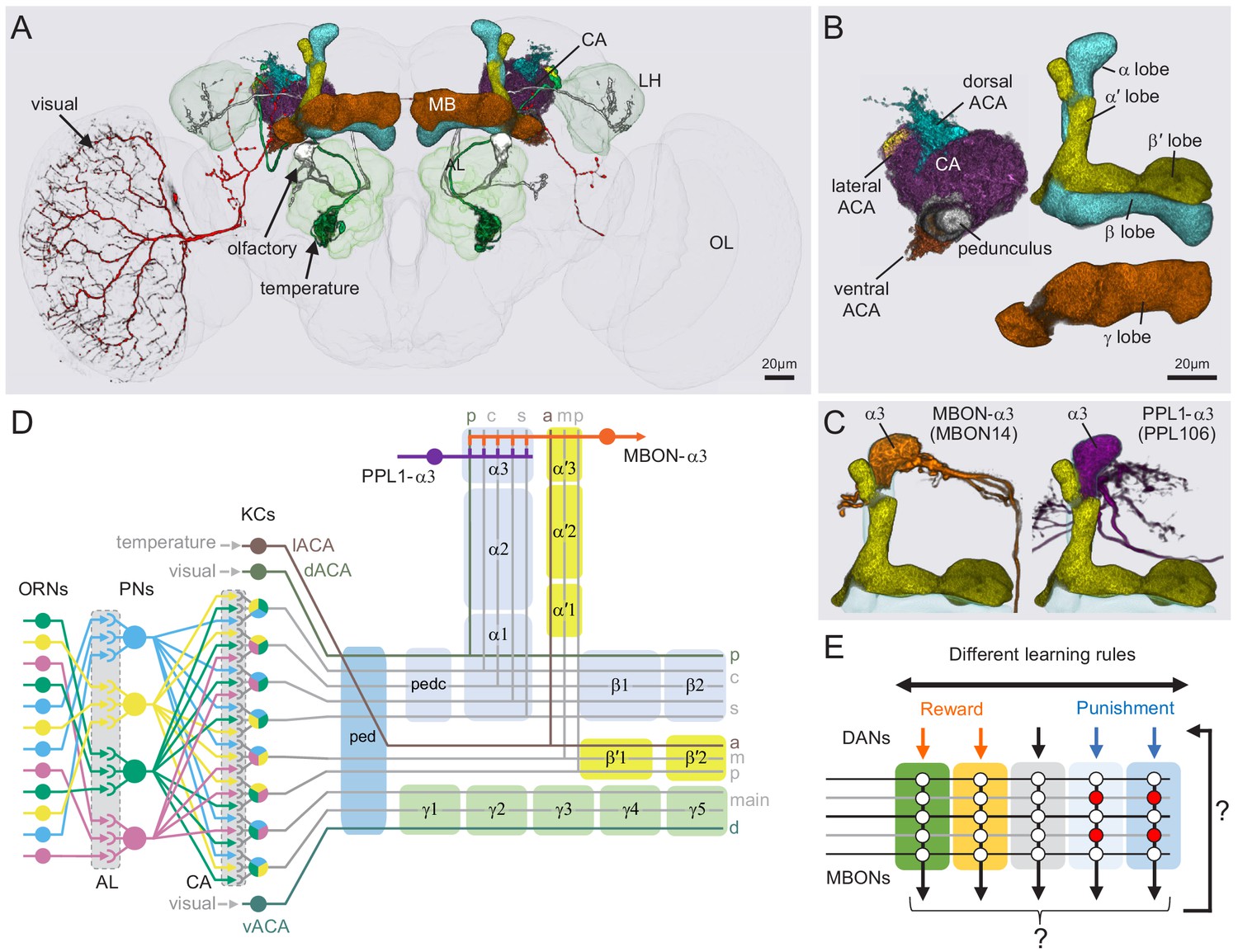
Anatomy of the adult Drosophila MB.
Diagram of structure and information flow in the MB. (A) An image of the brain showing subregions of the MB (see panel B for more detail) and examples of the sensory pathways that provide information to the KCs. Projection neurons (PNs) from the 51 olfactory glomeruli of the antennal lobe (AL) extend axons to the calyx (CA) of the MB and the lateral horn (LH). A total of 126 PNs, using a threshold of 25 synapses, innervate the CA and two innervate the lACA. Six olfactory PNs from the DL3 glomerulus are shown (white). Also shown is a visual projection neuron, aMe12 (red) that conveys information from the optic lobe (OL) to the ventral accessory calyx (vACA) and a thermosensory projection neuron (green) that conveys cold temperature information from arista sensory neurons in glomerulus VP3 to the lACA; the positions of the accessory calyces are shown in (B). See Figure 1—video 1 for additional details. (B) Subregions within the MB. The γ lobe, CA, and pedunculus are displayed separately from other lobes; their normal positions are as shown in panel A. Color-coding is as in panel A. (C) The MB output neuron (MBON14) whose dendrites fill the α3 compartment at the tip of the vertical lobe is shown along with the dopaminergic neuron (PPL106), whose axonal terminals lie in the same compartment. See Figure 1—video 2 for more detailed examples of the structure of a compartment. (D) A schematic representation of the key cellular components and information flow during processing of sensory inputs to the MB. Olfactory receptor neurons (ORNs) expressing the same odorant receptor converge onto a single glomerulus in the AL. A small number (generally 3 – 4) of PNs from each of the 51 olfactory glomeruli innervate the MB, where they synapse on the dendrites of the ~2000 Kenyon cells (KCs) in a globular structure, the CA. Each KC exhibits, on average, six dendritic ‘claws’, and each claw is innervated by a single PN. The axons of the KCs project in parallel anteriorly through the pedunculus (ped) to the lobes, where KCs synapse onto the dendrites of MB output neurons (MBONs). KCs can be categorized into three major classes α/β, α′/β′, and γ, based on their projection patterns in the lobes (Crittenden et al., 1998). The β, β′, and γ lobes constitute the medial lobes (also known as horizontal lobes), while the α and α′ lobes constitute the vertical lobes. These lobes are separately wrapped by ensheathing glia (Awasaki et al., 2008). The α/β and α′/β′ neurons bifurcate at the anterior end of the ped (pedc) and project to both the medial and vertical lobes (Lee et al., 1999). The γ neurons project only to the medial lobe. Dendrites of MBONs and terminals of modulatory dopaminergic neurons (DANs) intersect the longitudinal axis of the KC axon bundle, forming 15 subdomains or compartments, five each in the α/β, α′/β′, and γ lobes (numbered α1, α2, and α3 for the compartments in the α lobe from proximal to distal and similarly for the other lobes; Aso et al., 2014a; Tanaka et al., 2008). Additionally, one MBON and one DAN innervate the core of the distal pedunculus (pedc) intersecting the α/β KCs. In the current work, we further classified KCs into 14 types, 10 main types and four unusual embryonic born KCs, named KCγs1-s4 (see Figure 3); the main KC types have their dendrites in the main calyx, with the following exceptions: The dendrites of γd KCs form the ventral accessory calyx (vACA; Aso et al., 2009; Butcher et al., 2012); those of the α/βp KCs form the dorsal accessory calyx (dACA; Lin et al., 2007; Tanaka et al., 2008); and the dendrites of a subset of α′/β′ cells form the lateral accessory calyx (lACA) (Marin et al., 2020; Yagi et al., 2016). These accessory calyces receive non-olfactory input (Tanaka et al., 2008). Different KCs occupy distinct layers in the lobes as indicated (p: posterior; c: core; s: surface; a: anterior; m: middle, main and d: dorsal). Some MB extrinsic neurons extend processes only to a specific layer within a compartment. (E) Individual compartments serve as parallel units of memory formation (see Aso and Rubin, 2016). Reward or punishment is conveyed by dopaminergic neurons, and the coincidence of dopamine release with activity of a KC modifies the strength of that KC’s synapses onto the MBONs in that compartment. The circuit structure by which those MBONs combine their outputs to influence behavior and provide feedback to dopaminergic neurons are investigated in this paper.
Figure 2—figure supplement 1
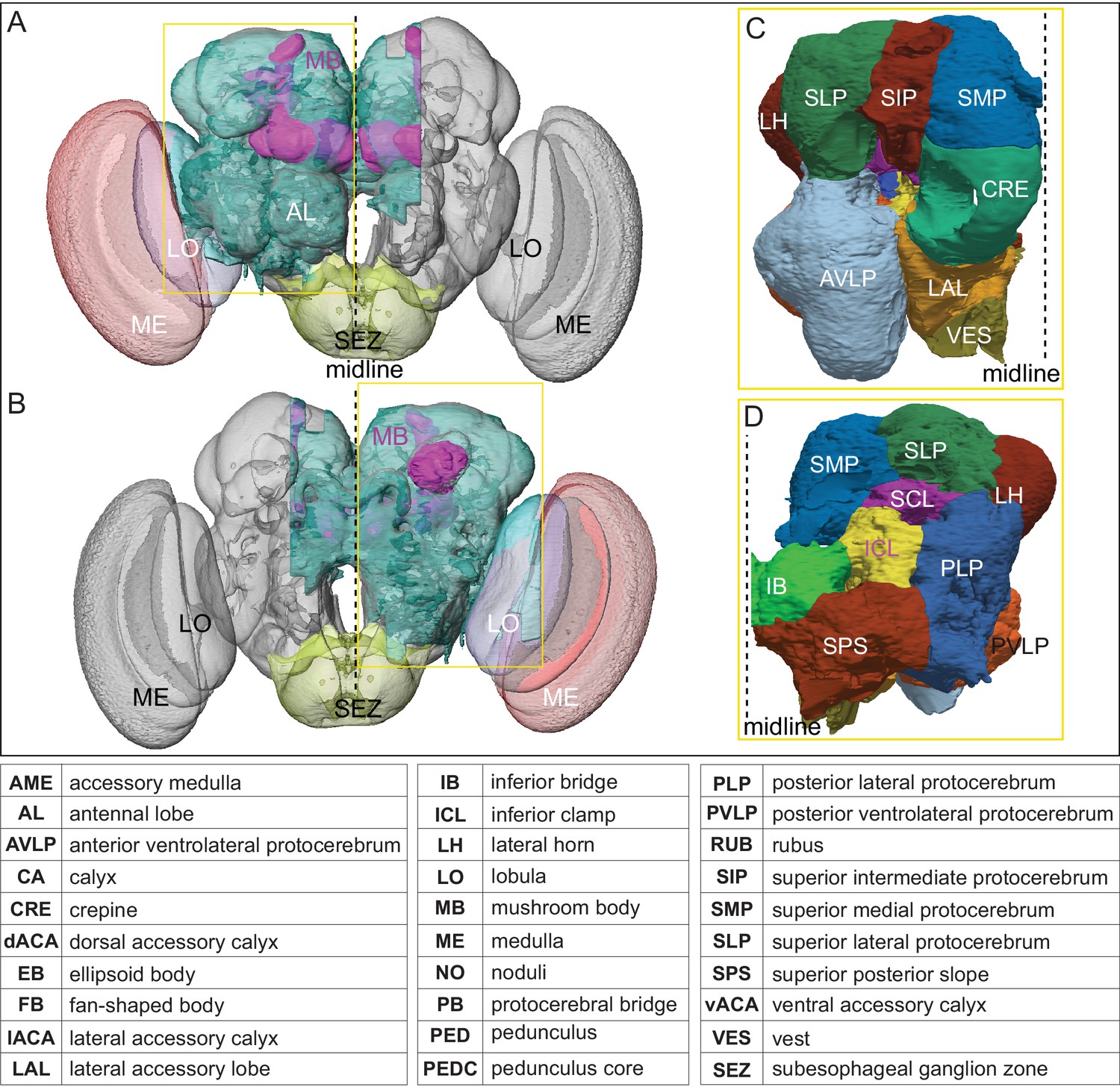
The extent of the hemibrain volume and key to brain area nomenclature.
(A) The portion of the central brain (light blue) that was imaged and reconstructed to generate the hemibrain volume (Scheffer et al., 2020) is superimposed on a frontal view of a grayscale representation of the entire Drosophila brain (JRC 2018 unisex template; Bogovic et al., 2018). The mushroom body (MB) is shown in purple. The midline is indicated by the dotted black line. The brain areas LO, ME, and SEZ, which largely lie outside the hemibrain, are labeled. (B) The same structures viewed from the posterior side of the brain. (C, D) Labeled brain regions in the area indicated by the yellow boxes in panels A and B, respectively. The table shows the abbreviations and full names for brain regions discussed in this paper. See Scheffer et al., 2020 for details.
Figure 3 with 4 supplements
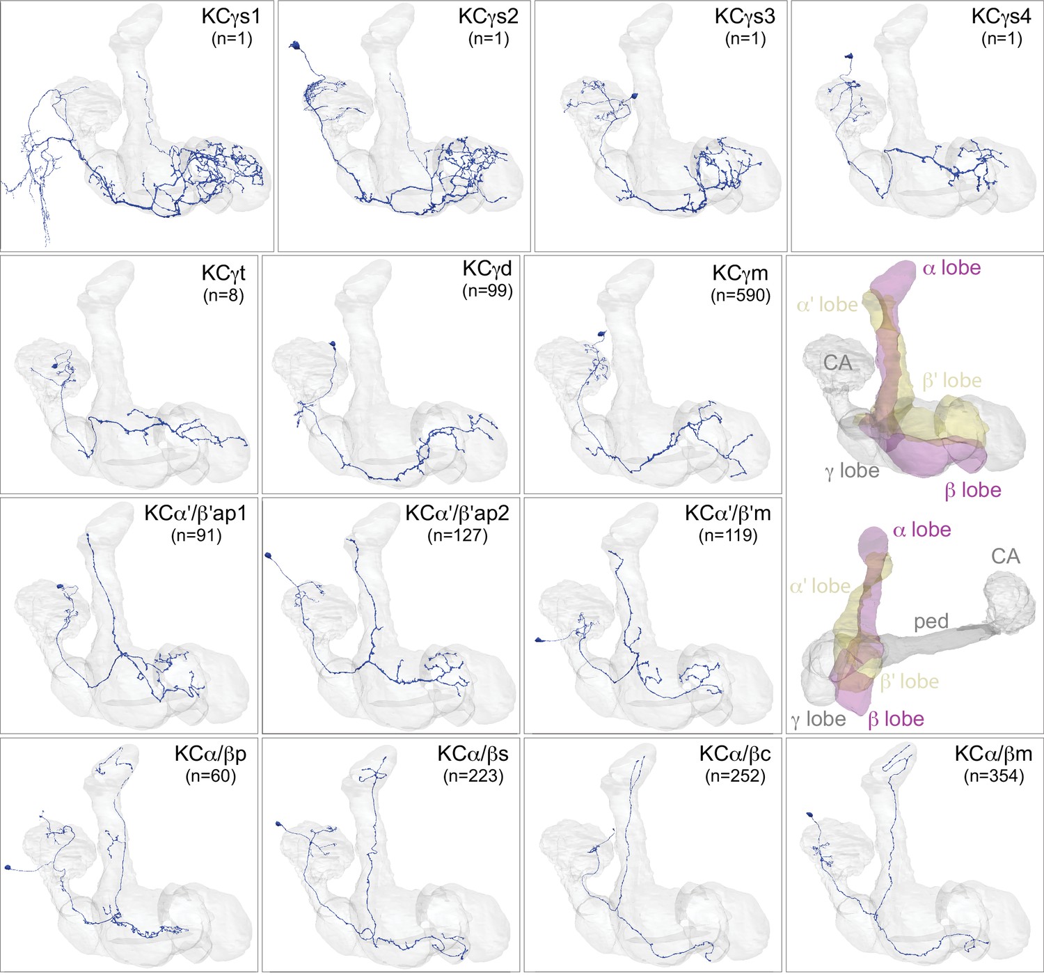
Kenyon cells.
Each panel shows a representative neuron of the indicated KC subtype together with the outline of the MB lobes and CA in gray , in a perspective view from an oblique angle to better display neuronal morphology. The insert on the right provides a key to the position of the individual lobes, the pedunculus (ped) and CA; the upper image presents the same view as KC subtype panels and the lower image shows a rotated view to better visualize the ped and CA. The numbers (n=) indicate the number of cells that comprise each KC subtype in this animal; the number of KCs is known to vary between animals (reviewed in Aso et al., 2009). Several of the KC subtypes are defined here for the first time, based on morphological clustering, as described in Figure 4. Although reconstruction of 78 KCα/β was incomplete in the CA as a consequence of a small area of reduced image quality, it did not affect morphological clustering, which was based on simplified axonal skeletons. More information about each of these cell types is shown in Figure 3—video 1. Additional intrinsic and extrinsic neurons with processes in the MB are shown in Figure 3—figure supplement 1.
Figure 3—figure supplement 1
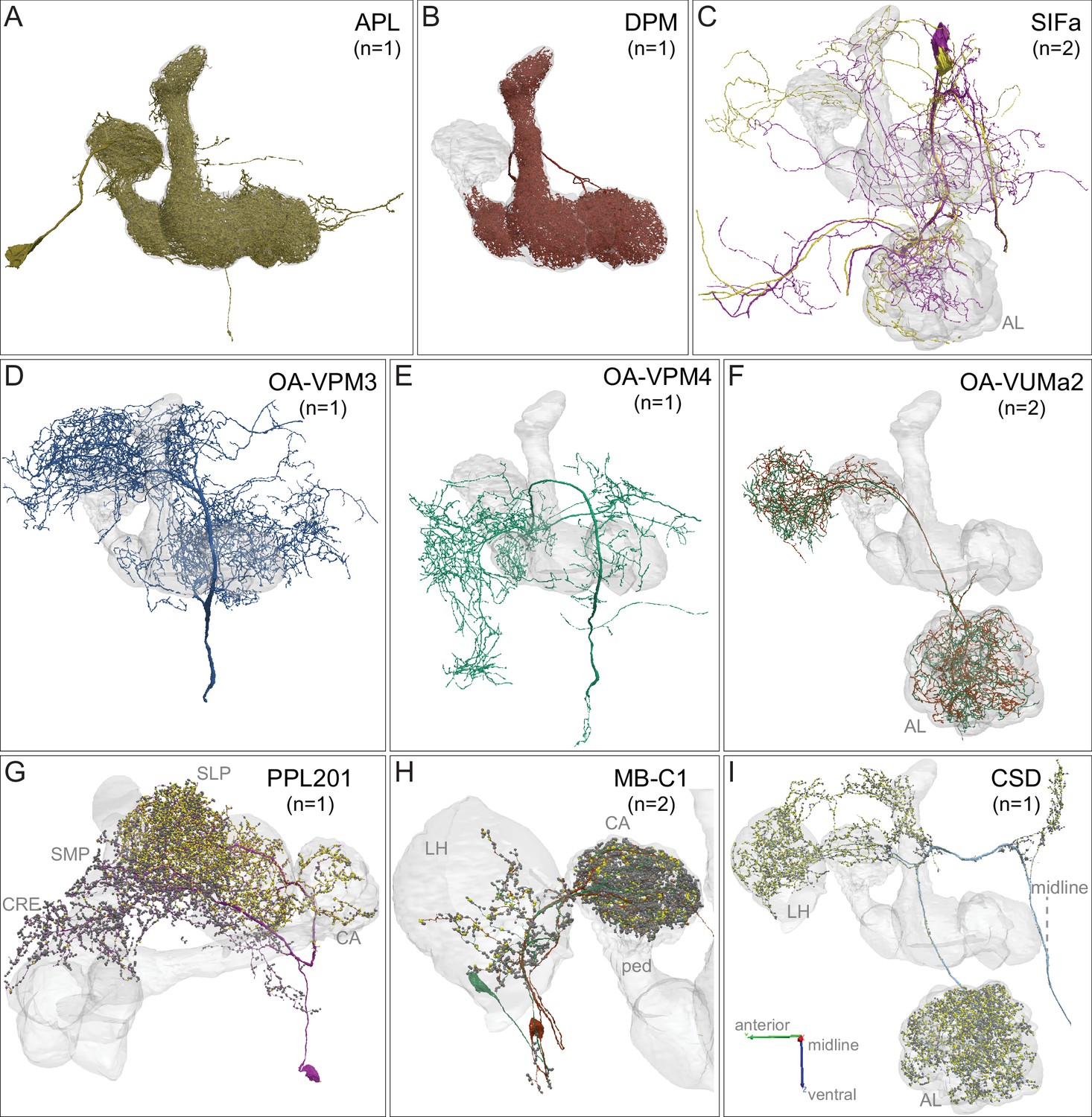
APL, DPM, SIFamide, OA-neurons and other modulatory neurons.
Neuronal morphologies are shown. (A) The anterior posterior lateral neuron, APL, innervates the entire MB (Figure 3—video 2). APL is GABAergic and provides negative feedback important for sparse coding of odor identities (Lin et al., 2014a; Liu and Davis, 2009; Papadopoulou et al., 2011; Tanaka et al., 2008). (B) The dorsal paired medial neuron, DPM, innervates the lobes in their entirety and the distal pedunculus (Figure 3—video 2). The DPM neuron has been proposed to use the neuropeptide amnesiac (Waddell et al., 2000), serotonin (Lee et al., 2011), and GABA (Haynes et al., 2015) as neurotransmitters and has been reported to be gap-junctionally coupled to APL (Wu et al., 2011). DPM has an important role in memory consolidation (Haynes et al., 2015; Keene et al., 2006; Pitman et al., 2011; Yu et al., 2005). The connectivity between DPM and APL and other neurons within the α lobe was described by Takemura et al., 2017, and our observations for the full MB are consistent with that description. (C) Two neurons that express the neuropeptide SIFamide, SIFa, are shown here and in Figure 3—video 3 (Park et al., 2014; Verleyen et al., 2004). (D–F) Three types of neurons that express the neurotransmitter octopamine (OA) are shown here and in Figure 3—video 3 (Busch et al., 2009; Aso et al., 2014a): (D) OA-VPM3, (E) OA-VPM4, and (F) OA-VUMa2. (G) PPL201 is a PPL2ab cluster dopaminergic neuron with axonal terminals in the CA, lateral horn (LH) and SLP; it has also been referred to as PPL2a (Mao and Davis, 2009; Tanaka et al., 2008; Zheng et al., 2018). In the CA, 16% of KCα/β as well as 25% of KCα′/β′ as well as KCγm neurons receives synapses from PPL201; however, KCs devoted to visual information are only very sparsely innervated (5% of KCα/βp and 3% of KCγd). The dendrites of this neuron are in the SMP and CRE. (H) Two GABAergic MB-C1 neurons (shown in different colors) innervate the LH and CA (Mao and Davis, 2009; Tanaka et al., 2008; Zheng et al., 2018). (I) The serotonergic CSD neuron innervates the AL, LH, and CA (Dacks et al., 2009). In panels G-I, yellow dots indicate presynaptic sites (sites where these neurons make synapses onto other neurons) and dark gray dots indicate postsynaptic sites (sites where these neurons receive input from other neurons).
Figure 3—video 1
KC types.
Figure 3—video 2
APL and DPM.
Figure 3—video 3
SIFamide and octopaminergic neurons.
Figure 4 with 5 supplements
Morphological hierarchical clustering reveals previously unrecognized KC subtypes.
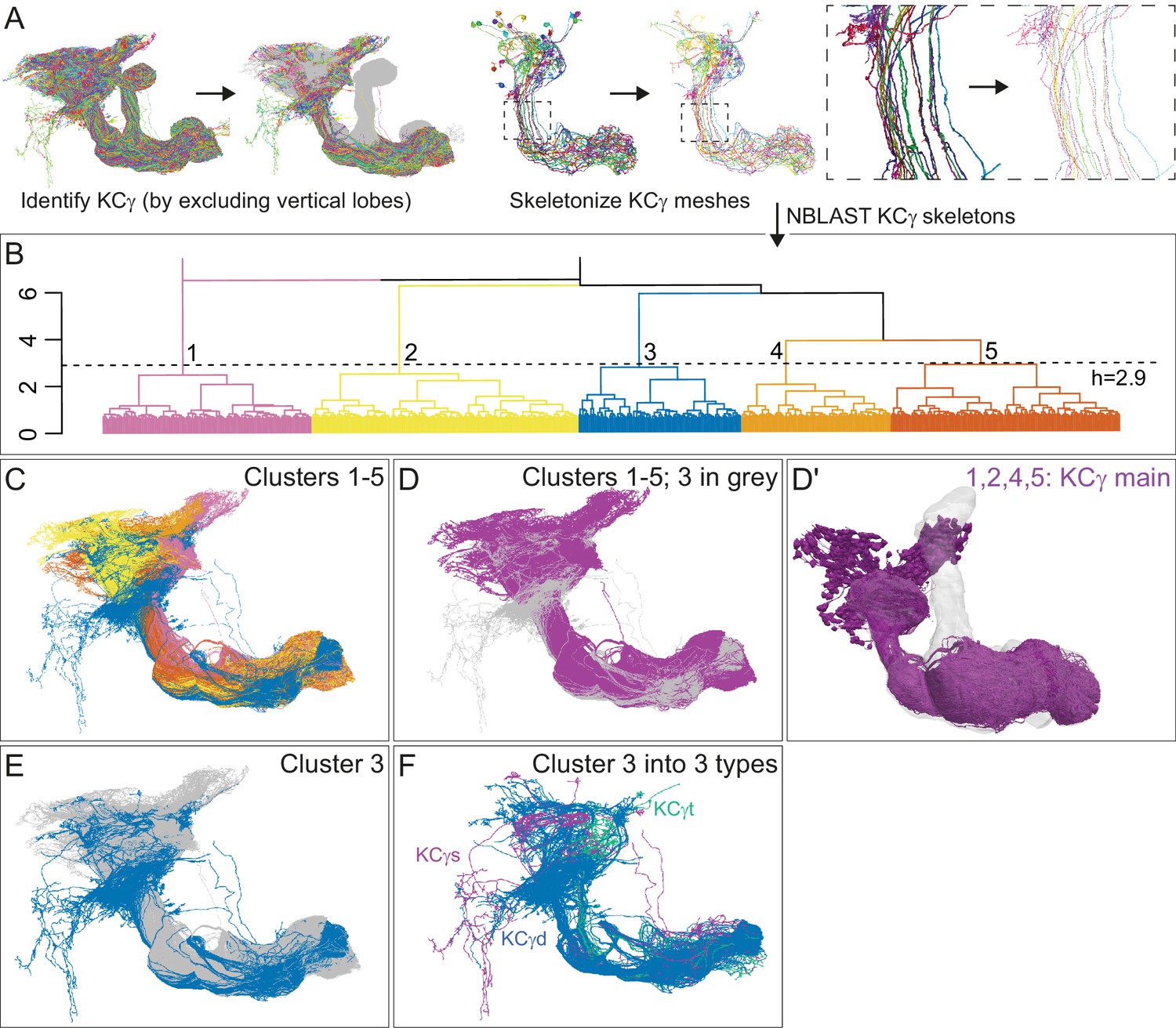
(A) KC typing workflow, using KCγ as an example. All γ KCs in the population of annotated KCs were identified by excluding all KCs with axons in the vertical lobes. The space filling morphologies of γ KCs were converted to skeletons (enlarged in the dashed box for clarity) and then NBLAST all-by-all neuron clustering (Costa et al., 2016) was used to reveal morphological groups. (B) Morphological hierarchical clustering of KCγ based on NBLAST scores is shown, cut at height 2.9 (dashed line), which produces five clusters. (C) KCγ skeletons of those five clusters are shown, color-coded as in (B). (D) KCγ skeletons in clusters 1, 2, 4, and 5, which includes all 590 KCγm, are shown in magenta; cluster 3 is shown in gray. (D′) Space filling morphologies of KCγm (clusters 1, 2, 4, and 5) shown in magenta with the MB in gray. (E) KCγ skeletons in cluster 3 (blue), which includes all KCγd, and clusters 1 – 2 and 4 – 5 (gray), which correspond to the KCγm type, are shown. (F) KCγ skeletons from cluster 3, cut at height 1.3, which produces six sub-clusters corresponding to three color-coded subtypes: green, 3.1 (eight KCγt); magenta, 3.2 (four KCγs); and blue, 3.3 – 3.6 (99 KCγd); see Figure 4—figure supplement 1 for details.
Figure 4—figure supplement 1
Successive rounds of whole neuron morphological hierarchical clustering reveal novel KCγ subtypes.
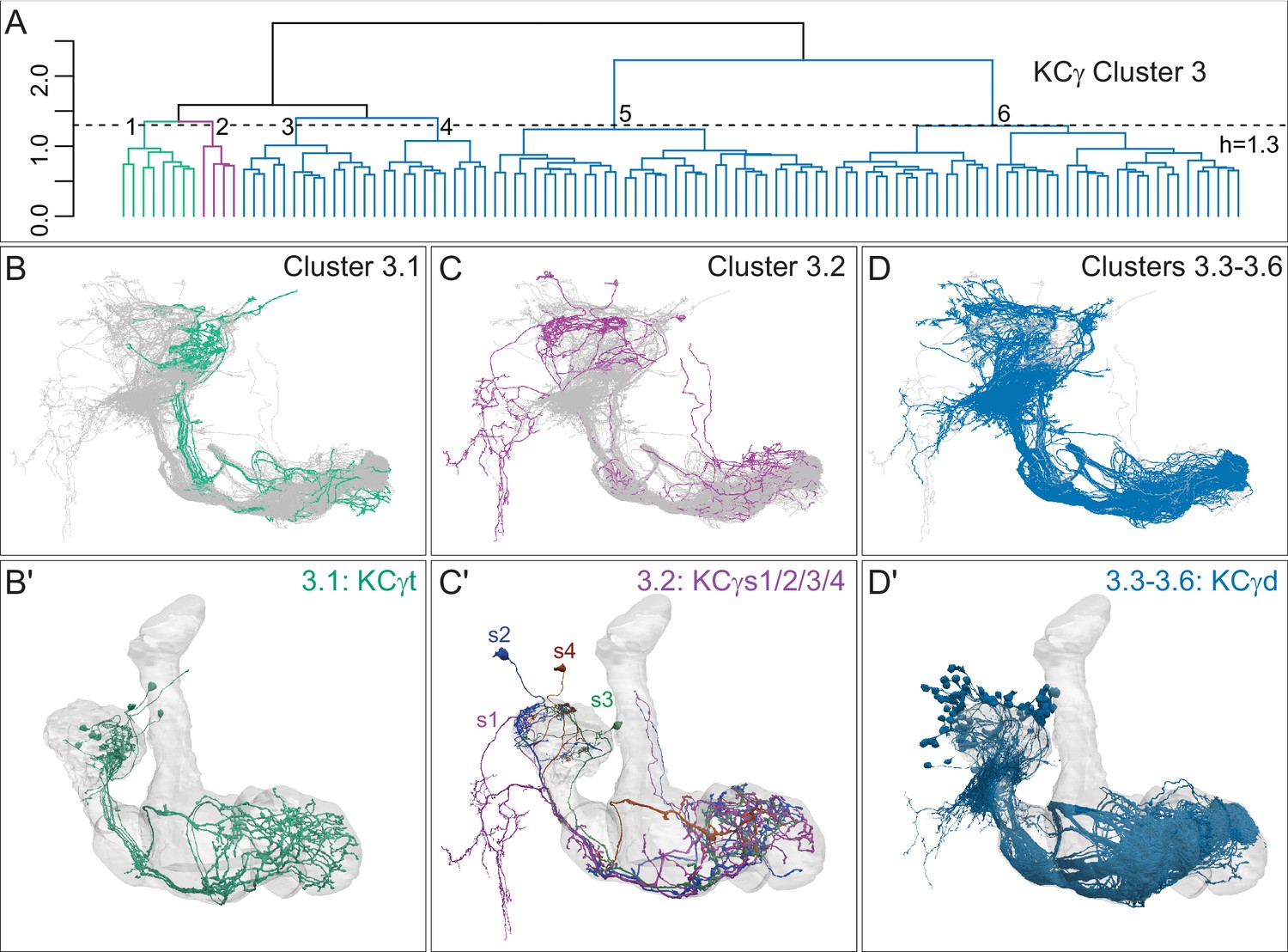
(A) Morphological hierarchical clustering based on NBLAST scores for all-by-all comparison of KCγ cluster 3 (from Figure 4B) cut at height 1.3 (dashed line); six sub-clusters are produced corresponding to three neuronal subtypes. (B) KCγt skeletons (cluster 3.1) shown in green, with remaining KCγ found in cluster 3 shown in gray. (B′) Space-filling morphologies of the same KCγt with the MB shown in gray. The eight KCγt neurons innervate the anterior of the CA, where most thermo/hygrosensory PNs project. (C) KCγs skeletons in cluster 3.2 shown in magenta, with remaining KCγ found in cluster 3 shown in gray. (C′) Space-filling morphologies of the four unique neurons of subtype KCγs, KCγs1/2/3/4, shown in magenta, dark blue, green, rust, respectively, with the MB shown in gray. Each KCγs likely derives from a different neuroblast. KCγs1 and KCγs2 both have unusually complex axons that wrap around the surface of the gamma lobe and feature a single dorsal branch; KCγs1 innervates all three accessory calyces and also exhibits a striking dendritic elaboration that extends into the PLP (Figure 10B), while KCγs2 has a large dendritic arbor in the lateral accessory calyx (lACA) and smaller dendritic branches in the ventroanterior CA (Marin et al., 2020 ; Figure 12—figure supplement 2C). KCγs3 and KCγs4 have axon morphologies more similar to those of canonical KCγ neurons, but KCγs3 receives input in the dorsal accessory calyx (dACA) and ventral accessory calyx (vACA), and KCγs4 receives input in the dACA and anterior CA. (D) KCγd dendrites innervate the vACA and their axons contribute to the dorsal layer of the γ lobe. The 99 KCγd found in sub-clusters 3.3, 3.4, 3.5, and 3.6 are shown in blue; the other γ KCs found in cluster 3 are shown in gray. (D′) Space-filling morphologies of the same γd KCs shown in blue, with the MB shown in gray.
Figure 4—figure supplement 2

Three distinct morphological subtypes of KCα′/β′.
(A) Morphological hierarchical clustering based on NBLAST scores for all-by-all comparison of α′/β′ KCs (simplified and pruned to include axon lobes only; black area in inset) is shown. When cut at height 2.0 (dashed line), α′/β′ KCs are split into three subtypes. (B) KCα′/β′ap1 skeletons from cluster 1 are shown in yellow with the remaining α′/β′ KCs shown in gray. (B′) Space-filling morphologies of the same KCα′/β′ap1 are shown in yellow, with the MB shown in gray. (C) KCα′/β′m skeletons from cluster 2 are shown in rust with the remaining α′/β′ KCs shown in gray. (C′) Space-filling morphologies of the same KCα′/β′m shown in rust, with the MB shown in gray. (D) KCα′/β′ap2 skeletons from cluster 3 are shown in dark blue with the remaining α′/β′ KCs shown in gray. (D′) Space-filling morphologies of the same KCα′/β′ap2 are shown in dark blue, with the MB shown in gray.
Figure 4—figure supplement 3
Further explanation of KC subtype nomenclature.
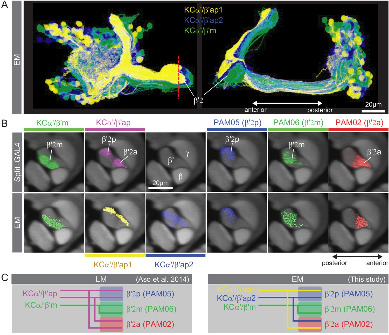
(A) Three subtypes of α′/β′ KCs in the hemibrain EM dataset are shown in the coordinates of the JF2018 standard brain in frontal (left) and sagittal view (right). The red dashed line indicates the position of the cross section of the MB β′ lobe shown in (B). (B) Innervation patterns of KCs and PAM DANs in the β′2 compartment. The reference neuropil stain from the JF2018 standard brain is shown in all panels in gray. Top: Two classes of KCs and three classes of PAM cluster DANs were defined by split-GAL4 drivers (Aso et al., 2014a) and light microscopic images of those split-GAL4 lines are shown: KCα′β′m, MB418B; KCα′β′ap, MB463B; reference neuropil stain; PAM05-β′2p, MB056B; PAM06-β′2m, MB032B; PAM02-β′2a, MB109B. Bottom: The positions of the indicated KC and PAM cell types are based on the hemibrain EM dataset, after transfer into the JF2018 standard brain coordinate system and color-coded. (C) Comparison of LM and EM datasets. Each α′β′ap bifurcates and innervates both β′2a and β′2p, coincident with the PAM02 and PAM05 innervation patterns, respectively. Morphological clustering revealed three classes of KCα′β′, subdividing α′β′ap into two classes: α′β′ap1 and α′β′ap2. KC α′β′ap1, KCα′β′ap2, and KCα′β′m likely correspond to KC α′β′a, KC α′β′m, and KCα′β′p, respectively, in Tanaka et al., 2008. However, we followed the nomenclature in Aso et al., 2014a to minimize confusion with established names based on split-GAL4 driver lines.
Figure 4—figure supplement 4
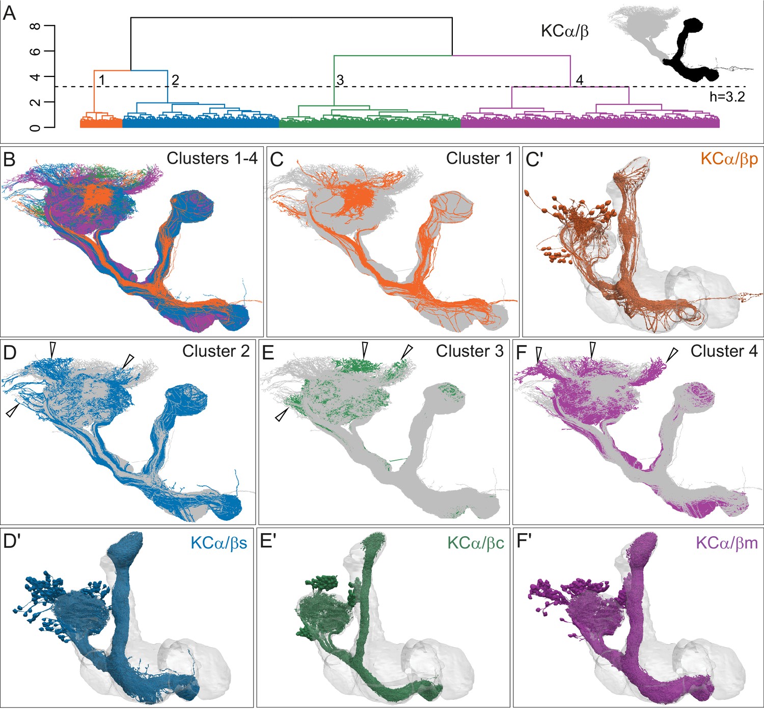
Four distinct morphological subtypes of KCα/β.
(A) Morphological hierarchical clustering based on NBLAST scores for all-by-all comparison of KCα/β carried out on that portion of their axons found in the lobes (black area in inset) is shown. When cut at height 3.2 (dashed line), α/β KCs are split into four subtypes. (B) KCα/β skeletons shown color-coded to match the clustering in (A). (C) KCα/βp, cluster 1, shown in rust, with the remaining α/β KCs shown in gray. (C’) Space-filling morphologies of the same KCα/βp shown in rust, with the MB shown in gray. (D) KCα/βs skeletons, cluster 2, shown in blue, with the remaining α/β KCs shown in gray. (D′) Space-filling morphologies of the same KCα/βs shown in blue, with the MB shown in gray. (E) KCα/βc skeletons, cluster 3, shown in green, with the remaining α/β KCs shown in gray. (E′) Space-filling morphologies of the same KCα/βc shown in green, with the MB shown in gray. (F) KCα/βm skeletons, cluster 4, shown in magenta, with the remaining α/β KCs shown in gray. (F′) Space-filling morphologies of the same KCα/βm shown in magenta, with the MB shown in gray. Distinct soma clusters are indicated by arrowheads in D, E, and F.
Figure 4—video 1
KC lineages.
Figure 5 with 2 supplements
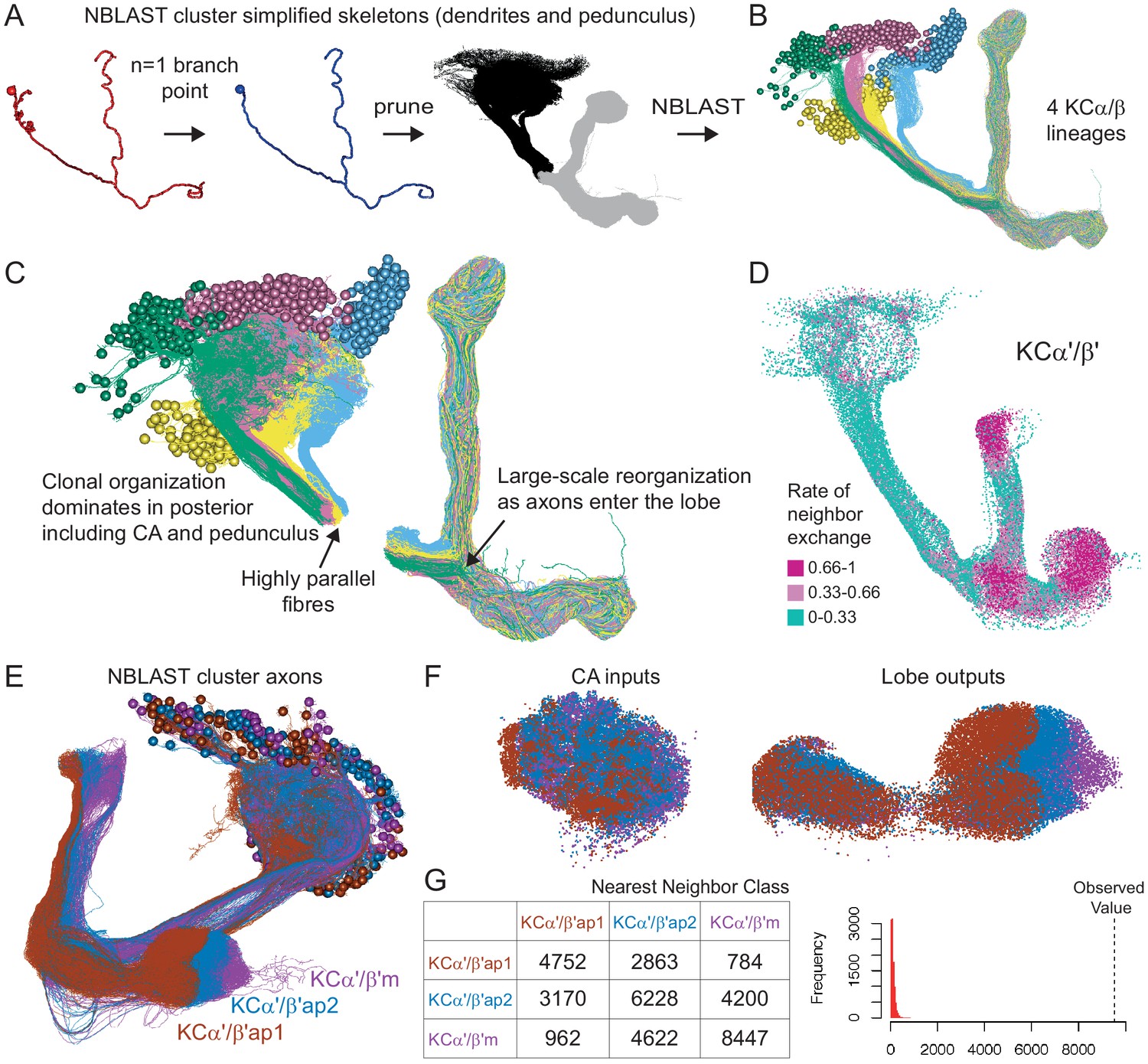
Organizational features of KC projections.
(A) KCs were simplified to skeletons with one major branch point which were used as input for NBLAST all-by-all whole neuron clustering. (B) This clustering revealed the four clonal units that make up the mushroom body (shown here for KCα/β). (C) Full neuronal morphologies of the four clusters show that the positions of the neurons in the CA are strongly influenced by this fourfold clonal unit structure, which is also reflected in the arrangement of the highly parallel fibers in the pedunculus. On entering the lobes, the axons reorganize, and the neurons from the four clusters become intermingled. (D) Visualization of the rate of change in KC neighbors quantified as the fraction of 10 nearest neighbors that change compared with a position 5 µm closer to the soma. Large values imply a rapid change in the neighbors of individual KC fibers, which is observed at the entry and tips of the KCα′/β′ lobe as illustrated here. Figure 5—figure supplement 1B shows similar visualizations for the KCγ and KCα/β lobes; rapid change in neighbors is seen throughout the KCγ lobe while KCα/β neurons show an intermediate rate of change. (E) NBLAST clustering of the axons of α′/β′ KCs reveals three clear laminae in the vertical and horizontal lobes, which correlate with a layered organization in the CA and correspond to the three KC α′/β′ subtypes. (F) A similar organization is seen for KCα′/β′ dendrites in the CA and axon outputs in the lobes. (G) As a statistical test for the correlated lobe/CA organization into three subtypes, each synapse in the CA was matched with its closest neighbor from another neuron and the subtype of that neighbor recorded. The contingency table (left) shows that nearest neighbor synapses were most commonly from the same subtype. A permutation test (n = 10,000) confirmed that this statistic was far higher than expected by chance (right).
Figure 5—figure supplement 1

Additional organizational features of KC projections.
(A) Posterior view of the CA showing the four clonal units that make up α′/β′ KCs (Figure 5B) as revealed by NBLAST clustering (Figure 5A). (B) Visualization of the rate of change in KC neighbors quantified as the fraction of 10 nearest neighbors that change compared with a position 5 mm closer to the soma. Large values imply a rapid change in the neighbors of individual KC fibers, which are observed all the way along γm KCs in the γ lobe; much lower rates of rearrangement are seen in the pedunculus and in segments of the α/β KCs in the vertical lobe. (C) Cross-sections through the mushroom body pedunculus, at the point indicated by the hollow arrowhead, showing the organization of KC types by birth order as indicated by the hollow arrows, with the first-born types (KCγs and KCγd) generally more peripheral and the last-born type (KC α/β) more central.
Figure 5—figure supplement 2
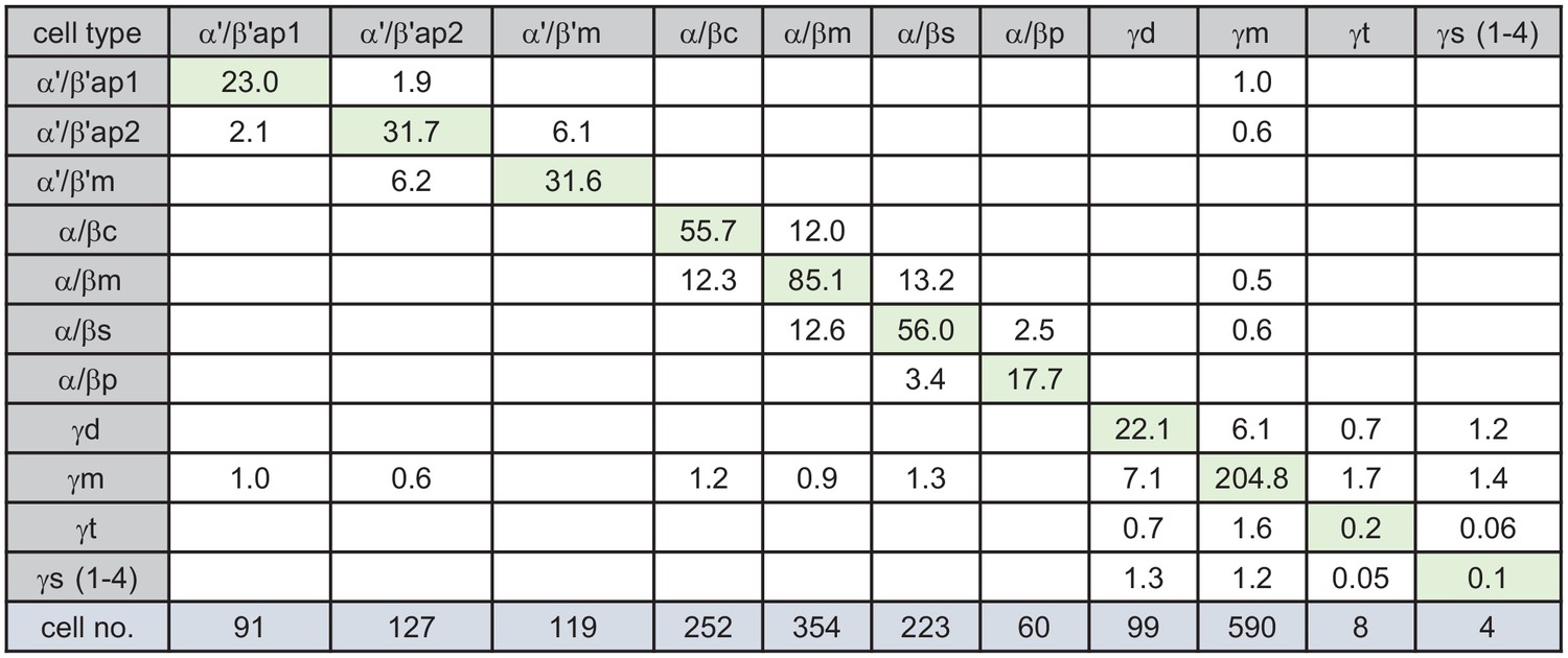
KC-to-KC synapses.
The total number of synapses/1000 made between the indicated KC types in the MB (including the lobes, pedunculus, and calyces) are shown. Only connections totaling > 500 synapses are shown, except for those involving γt and γs where connections less than 50 synapses were included because of the small numbers of cells of these types. The four γs cell types were pooled. The y-axis shows postsynaptic cell types and the x-axis presynaptic cell types. The number of KCs of each type is shown.
Figure 6 with 3 supplements
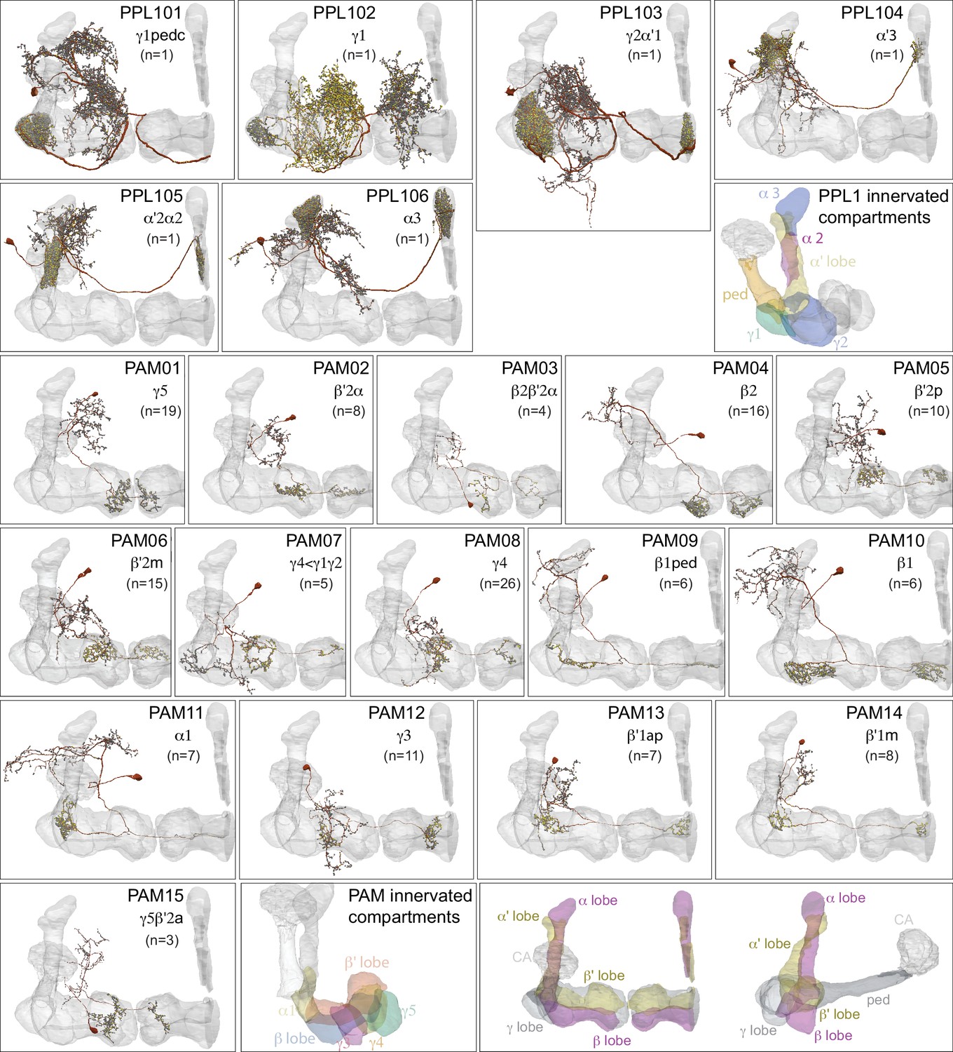
Dopaminergic neurons (DANs).
Each panel shows a DAN cell type, with its name, the compartment(s) it innervates and the number of cells of that type per brain hemisphere indicated; the outline of the MB lobes and CA are shown in gray , in a perspective view from an oblique angle to better display neuronal morphology. Figure 6—figure supplement 1 shows which DANs, MBONs, and KCs are found in each compartment. PPL1 dopaminergic neurons are divided into six cell types, PPL101, PPL102, PPL103, PPL104, PPL105, and PPL106. As a population, the PPL1 neurons innervate the α' lobe, α lobe compartments 2 and 3, and γ lobe compartments 1 and 2, as illustrated. There is only one PPL1 DAN of each type per hemisphere, but they send their axons bilaterally to innervate the same MB compartments, although less densely, in the other brain hemisphere (see Aso et al., 2014a). PPL102 differs in morphology and polarity from the other PPL1 DANs and is likely to perform different functions. For this reason, it has not been included in certain analyses of DANs. All other compartments are innervated by PAM DANs, as illustrated: PAM01, PAM02, PAM03, PAM04, PAM05, PAM06, PAM07, PAM08, PAM09, PAM10, PAM11, PAM12, PAM13, PAM14, and PAM15. Unlike the PPL1 DANs, multiple PAM DANs of the same cell type innervate the same compartment, and in some cases the same compartment has different PAM DAN types innervating different subdomains of the compartment. MB lobes are shown in gray. A single representative neuron is shown for each cell type in magenta, with gray dots indicating postsynaptic sites and yellow dots indicating presynaptic sites. Images showing the identity of the MB lobes are shown in the lower right.
Figure 6—figure supplement 1
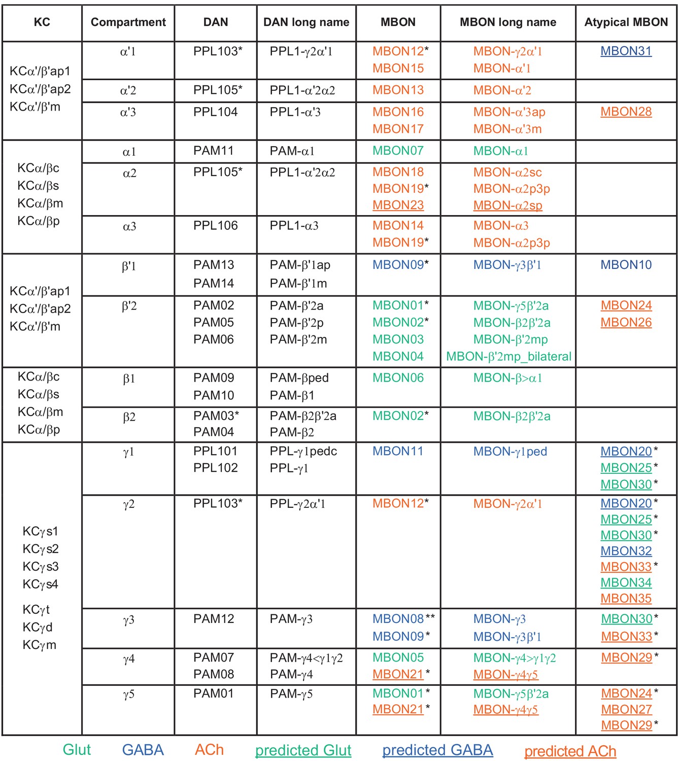
Table of cell types found in each MB compartment.
This table shows which KCs, DANs, and MBONs are found in each of the 15 compartments of the MB lobes. Both the short names used throughout this paper and the longer names used in Aso et al., 2014a are shown. MBONs or DANs that innervate more than one compartment are marked with an asterisk. MBON names are color-coded based on neurotransmitter. MBONs whose neurotransmitter assignment is based on prediction (Eckstein et al., 2020) are underlined.
Figure 6—figure supplement 2
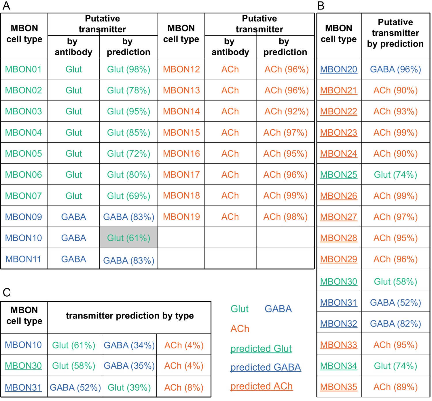
MBON neurotransmitter predictions.
(A) Neurotransmitters of typical MBONs previously determined by antibody staining (Aso et al., 2014a) are compared to computational predictions (Eckstein et al., 2020). In 17 of 18 cases they agree; the exception is MBON10. (B) Predicted neurotransmitter for MBONs for which antibody staining information is lacking. The percentage indicates the fraction of individual synapses scored that agreed with the overall prediction. See Eckstein et al., 2020 for details. Note that predictions for acetylcholine are particularly robust. (C) Three MBON types, including MBON10, have less than a 70% prediction for their most likely neurotransmitter and their second and third most likely transmitters are shown. Note that if glutamate is assumed to be inhibitory, even these ambiguous predictions can distinguish inhibitory from excitatory transmitters with high confidence.
Figure 6—figure supplement 3
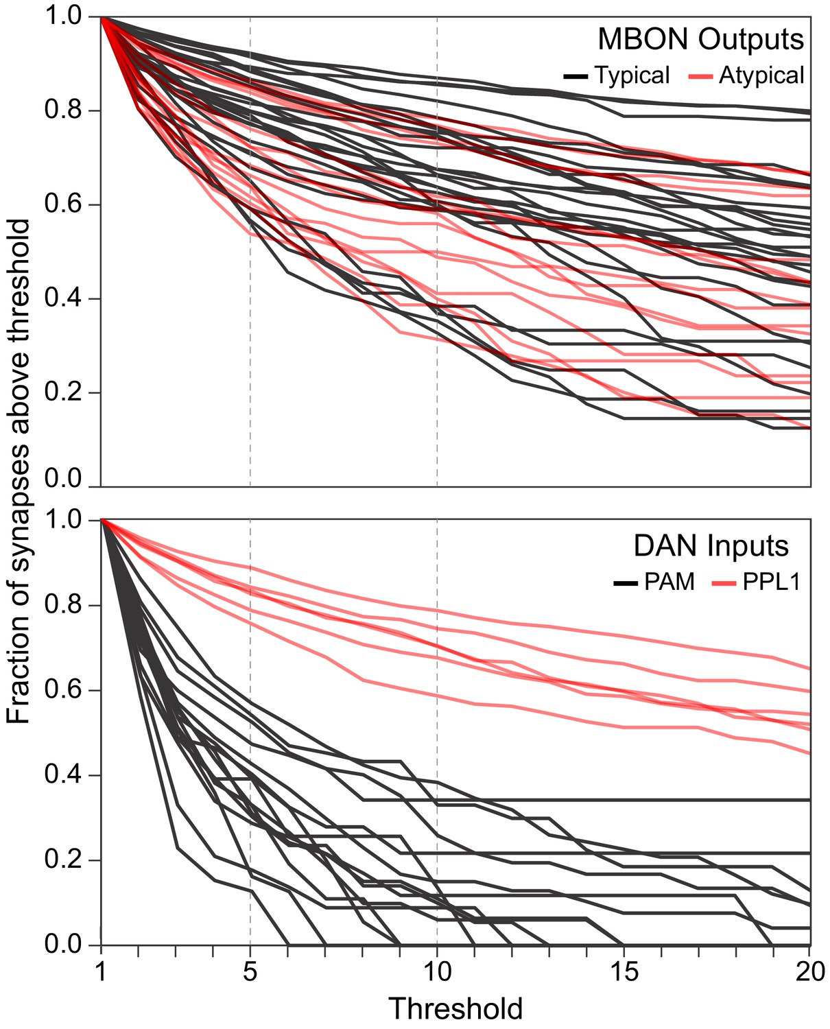
Synapse number distribution for MBON outputs and DAN inputs.
The plots show the fraction of synapses that would fall above thresholds ranging from 1 to 20 synapses. The upper plot shows a line for each MBON, with typical MBONs in black and atypical MBONs is red. The lower plot shows a line for each PPL1 DAN in red and a line for every tenth (based on total synapse number) PAM DAN. Dotted lines are shown at threshold values of 5 and 10.
Figure 7
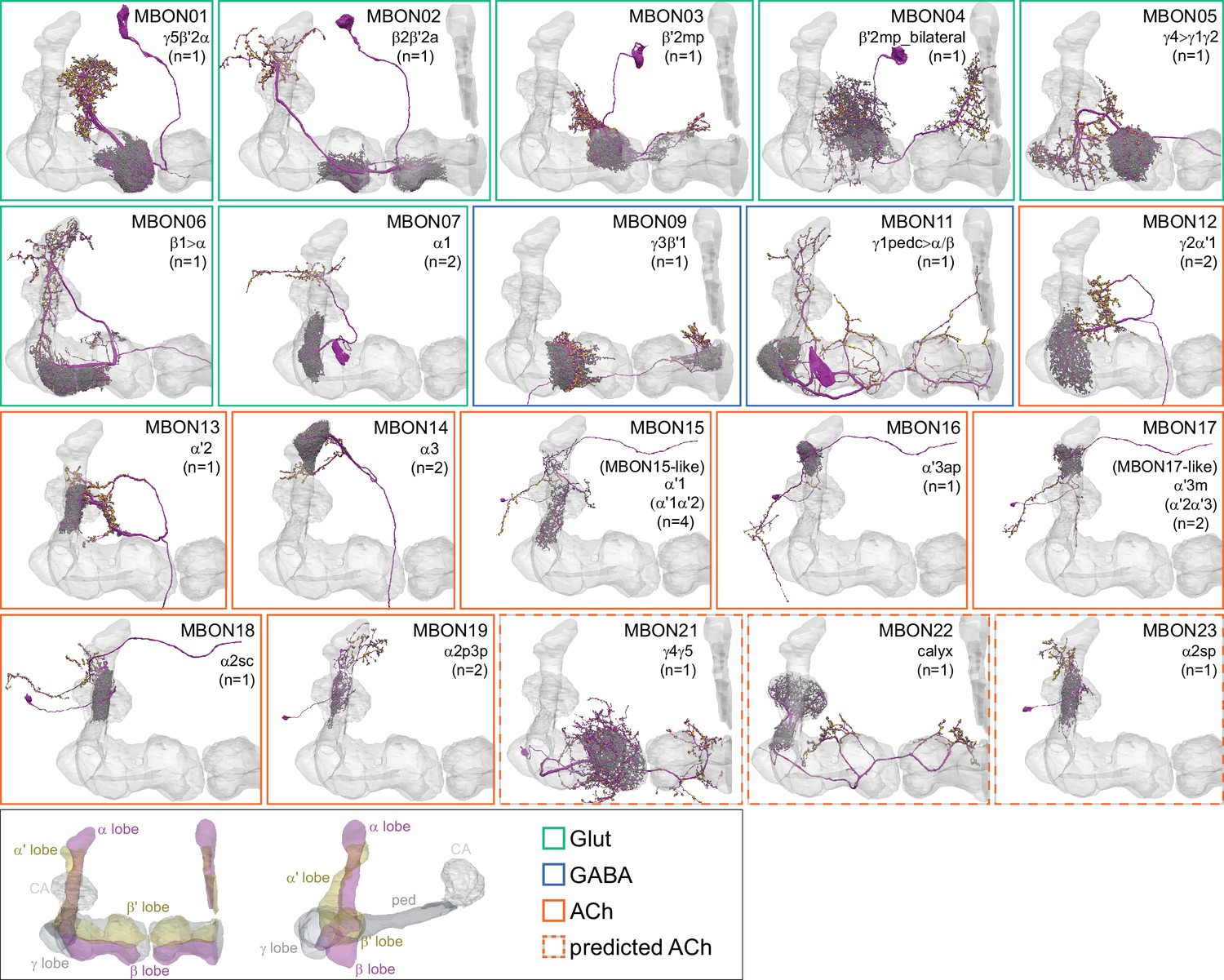
Mushroom Body Output Neurons (MBONs).
Each panel shows one of the previously described 20 types of MBONs, with its name, the compartment(s) it innervates and the number of cells of that type per brain hemisphere indicated (Aso et al., 2014a; Takemura et al., 2017); the outline of the MB lobes and CA are shown in gray, in a perspective view from an oblique angle to better display neuronal morphology. MB lobes are shown in gray. A single representative neuron is shown for each cell type (magenta), with gray and yellow dots indicating postsynaptic and presynaptic sites, respectively. The bounding box for each neuron is color-coded by the neurotransmitter used by that MBON; dashed boxes are used where the transmitter type is based on computational prediction (see Figure 6—figure supplement 2). The lower panel shows the neurotransmitter color code as well as diagrams of the MB in which the different lobes are indicated; the left diagram is in the same orientation as the other panels. These MBONs are considered to be typical in that their dendritic arbors are confined to the MB lobes. We reclassified MBON10 and MBON20 (Aso et al., 2014a) as atypical MBONs since their dendrites extend outside the MB lobes. MBON08, defined by split-GAL4 line MB083C (Aso et al., 2014a), was not found in the hemibrain volume. For the other 21 MBON types, we found only minor differences with previous studies (Aso et al., 2014a; Takemura et al., 2017). For example, MBON15 (α′1) and MBON17 (α′3m), which each were described as having two cells in Aso et al., 2014a; Takemura et al., 2017 , had additional cells in the hemibrain that were similar in morphology, but had some connectivity differences, that we refer to as MBON15-like and MBON17-like. However, since our observations are based on a single individual, we did not split them into separate cell types. Links to the neuPrint records of these MBON types are as follows: MBON01, MBON02, MBON03, MBON04, MBON05, MBON06, MBON07, MBON09, MBON11, MBON12, MBON13, MBON14, MBON15 (including MBON15-like), MBON16, MBON17 (including MBON17-like), MBON18, MBON19, MBON21, MBON22, and MBON23.
Figure 8 with 29 supplements
Atypical MBONs.
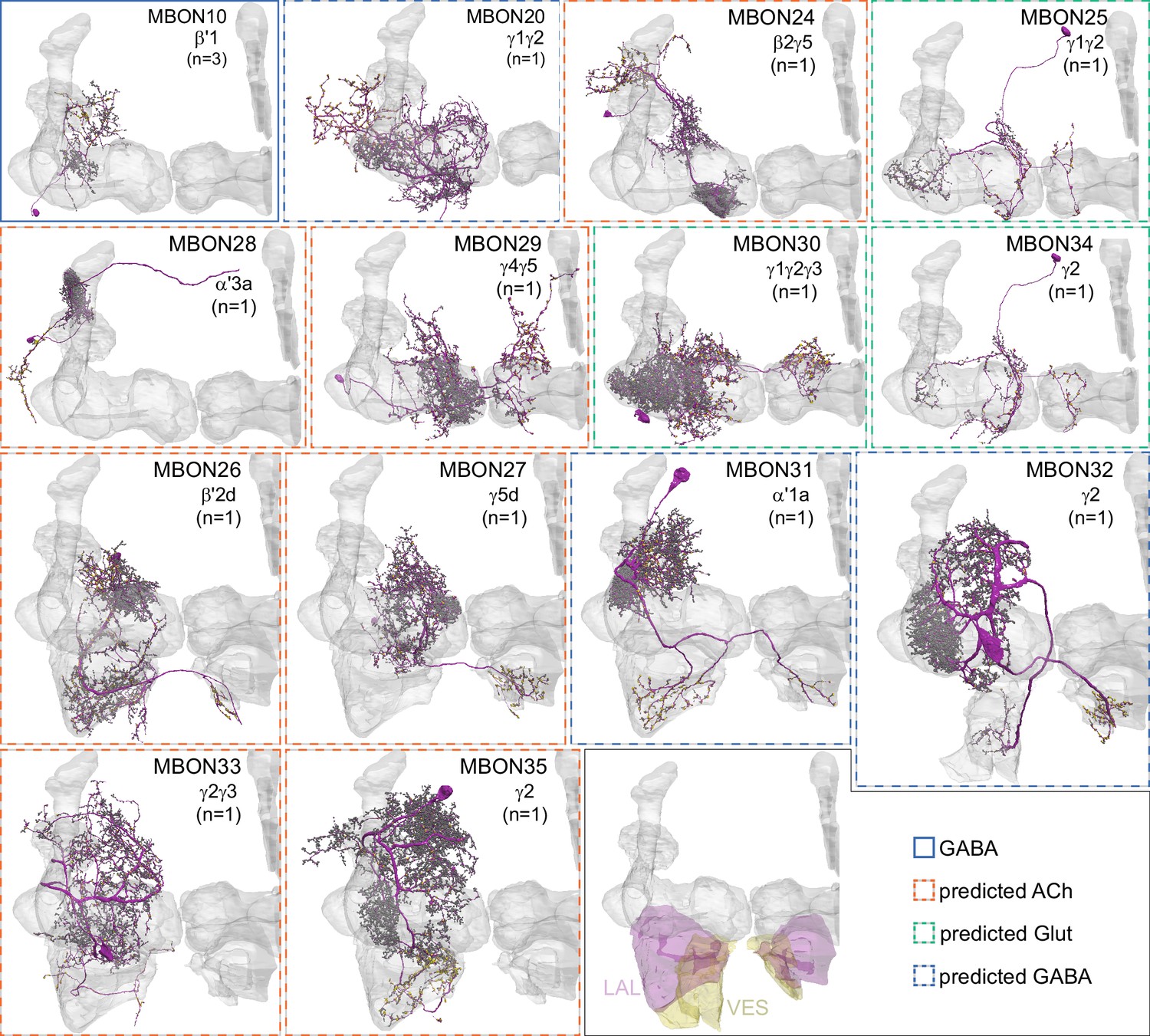
Each panel shows one of the 14 types of atypical MBONs, with its name, the compartment(s) it innervates and the number of cells of that type per brain hemisphere indicated. Figure 6—figure supplement 1 shows which DANs, MBONs, and KCs are found in each compartment. MB lobes are shown in gray and in the bottom right panel the lateral accessory lobe (LAL) and vest (VES) brain areas are highlighted. Neuronal morphologies are shown with dark gray dots and yellow dots indicating postsynaptic and presynaptic sites, respectively. The MBONs shown in this figure are considered to be atypical in that their dendritic arbors are only partially within the MB lobes. Twelve of these types were discovered in the course of the current study. The other two, the GABAergic MBON10 and MBON20, were described by Aso et al., 2014a, but we have reclassified them here as atypical MBONs because they have dendrites both inside and outside the MB lobes. The three MBON10s in the EM volume have 69 , 68, and 50% of their postsynaptic sites outside the MB lobes; one is shown here. All the other atypical MBONs occur once per hemisphere. Unlike most typical MBONs that innervate brain areas that are dorsal to the MB, six of the atypical MBONs innervate areas that are ventral to the MB. The LAL is a target of several atypical MBONs, and one also innervates the VES. More detailed information about each of the atypical MBONs can be found in Figure 8—figure supplements 1–14 and Figure 8—videos 1–14. Figure 8—figure supplement 15 compares the non-MB inputs to these MBONs. The bounding box for each MBON is color-coded by the neurotransmitter used by that MBON; dashed boxes are used where the transmitter type is based on computational prediction (see Figure 6—figure supplement 2). Links to the neuPrint records of these MBON types are as follows: MBON10, MBON20, MBON24, MBON25, MBON26, MBON27, MBON28, MBON29, MBON30, MBON31, MBON32, MBON33, MBON34, and MBON35.
Figure 8—figure supplement 1
Atypical MBON10.
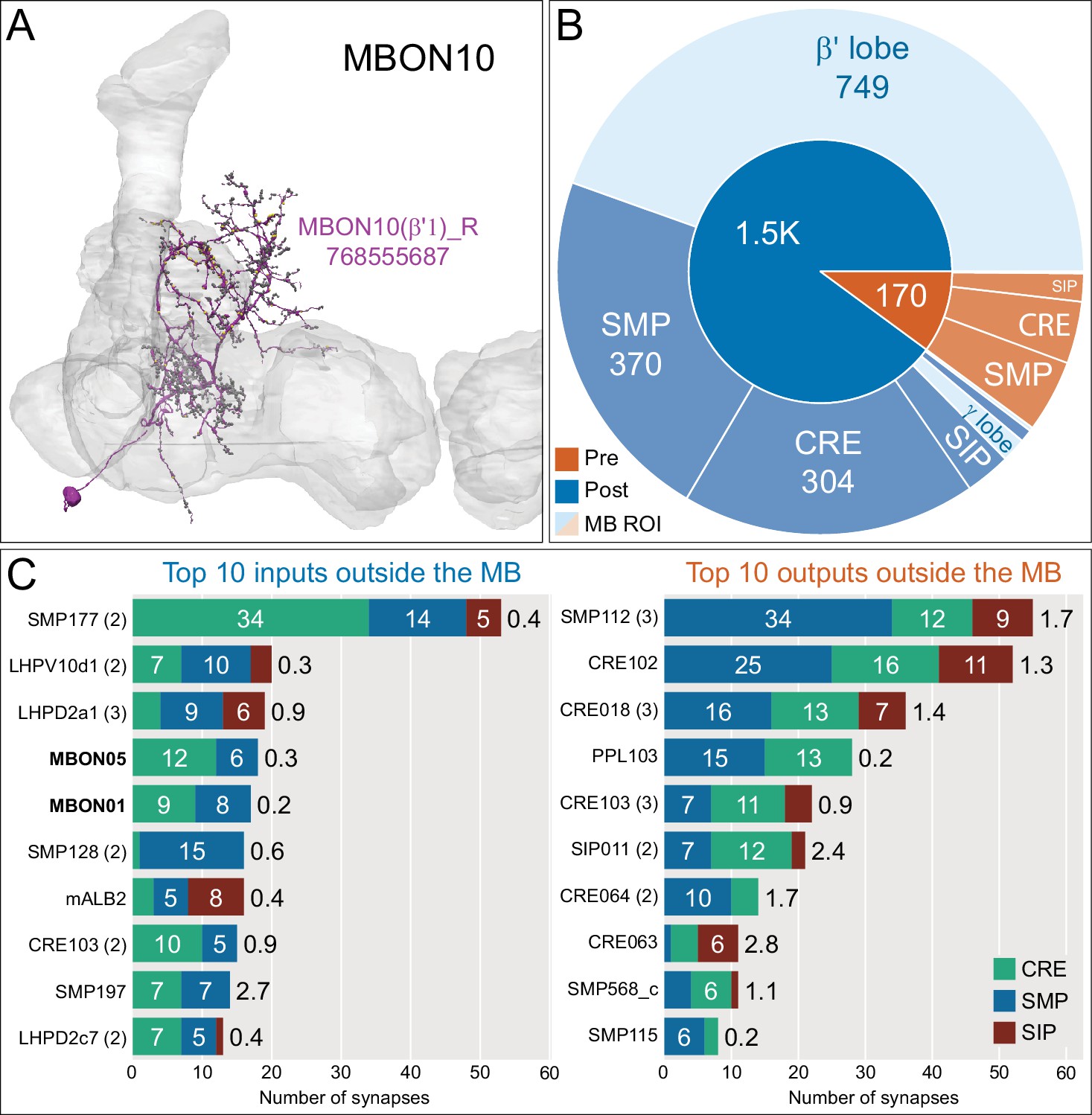
(A) Atypical MBON10 is the only atypical MBON cell type with more than one cell per brain hemisphere. One of the three MBON10s is shown here; all three cells are shown in Figure 8—video 1. Presynaptic sites are shown in yellow and postsynaptic sites are shown in gray. (B) A pie chart showing the distribution of MBON10’s presynaptic sites (indicated in orange) and postsynaptic sites (in blue). The inner circle shows the total number of MBON10’s pre- and postsynaptic sites; the numbers represent the MBON10 shown in A. The outer circle of the pie chart shows the brain regions in which these sites occur; regions of the MB are shown in lighter colors. (C) MBON10’s top 10 inputs (left) and outputs (right) outside the MB lobes are shown by neuron type as bar charts. The numbers in each row represent synapse numbers and the brain regions in which these synapses occur are color- coded. (Left) T he numbers next to each row indicate the percentage of that neuron’s synaptic output that goes to MBON10. Note that two typical MBONs synapse onto MBON10, MBON01 (γ5β'2a), and MBON05 (γ4>γ1γ2). Links to these cell types in neuPrint are: SMP177, LHPV10d1, LHPD2a1, MBON05, MBON01, mALB2, SMP128, CRE103, SMP197, and LHPD2c7. (Right) T he numbers next to each row indicate the fraction of that neuron's input that is provided by MBON10. Links to these cell types in neuPrint are: SMP112, CRE102, CRE018, PPL103, CRE103, SIP011, CRE064, SMP568_c, CRE063, and SMP115.
Figure 8—figure supplement 2
Atypical MBON20.
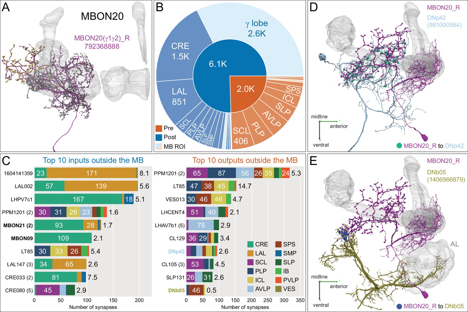
(A) Atypical MBON20 (γ1γ2) is shown here and in Figure 8—video 2. Presynaptic sites are shown in yellow and postsynaptic sites are shown in gray. MBON20 receives 45% of its input from sites within MB lobes and 85% of those input are in the γ1γ2 compartments. (B) A pie chart showing the distribution of MBON20’s presynaptic sites (indicated in orange) and postsynaptic sites (in blue). The inner circle shows the total number of MBON20’s pre- and postsynaptic sites. The outer circle of the pie chart shows the brain regions in which these sites occur; regions of the MB are shown in lighter colors. (C) MBON20’s top 10 inputs (left) and outputs (right) outside the MB lobes are shown by neuron type as bar charts. The numbers in each row represent synapse numbers and the brain regions in which these synapses occur are color- coded. (Left) T he numbers next to each row indicate the percentage of that neuron’s synaptic output that goes to MBON20. Links to these cell types in neuPrint are: 1604141359, LAL002, LHPV7c1, PPM1201, MBON21, MBON09, LT85, LAL147, CRE033, and CRE080. (Right) T he numbers next to each row indicate the fraction of that neuron's input that is provided by MBON20. Links to these cell types in neuPrint are: PPM1201, LT85, VES013, LHCENT4, LHAV7b1, CL129, DNp42, CL105, SLP131, and DNb05. Neuron names in colored text indicate neurons further discussed in panel D and E and are color-coded to match the neurons in these panels. Note MBON20 makes strong reciprocal connections with LT85, which is a LO tangential neuron conveying visual information, and PPM1201. (D, E) Although not all DNs have been identified, there are at least two individual DNs that are strongly connected to MBON20. (D) DNp42, connects to MBON20 with 94 synapses in dorsal brain regions, including SCL and PLP. (E) DNb05, connects to MBON20 with 57 synapses in SPS. Note DNb05 also receives input from PNs in the AL.
Figure 8—figure supplement 3
Atypical MBON24.
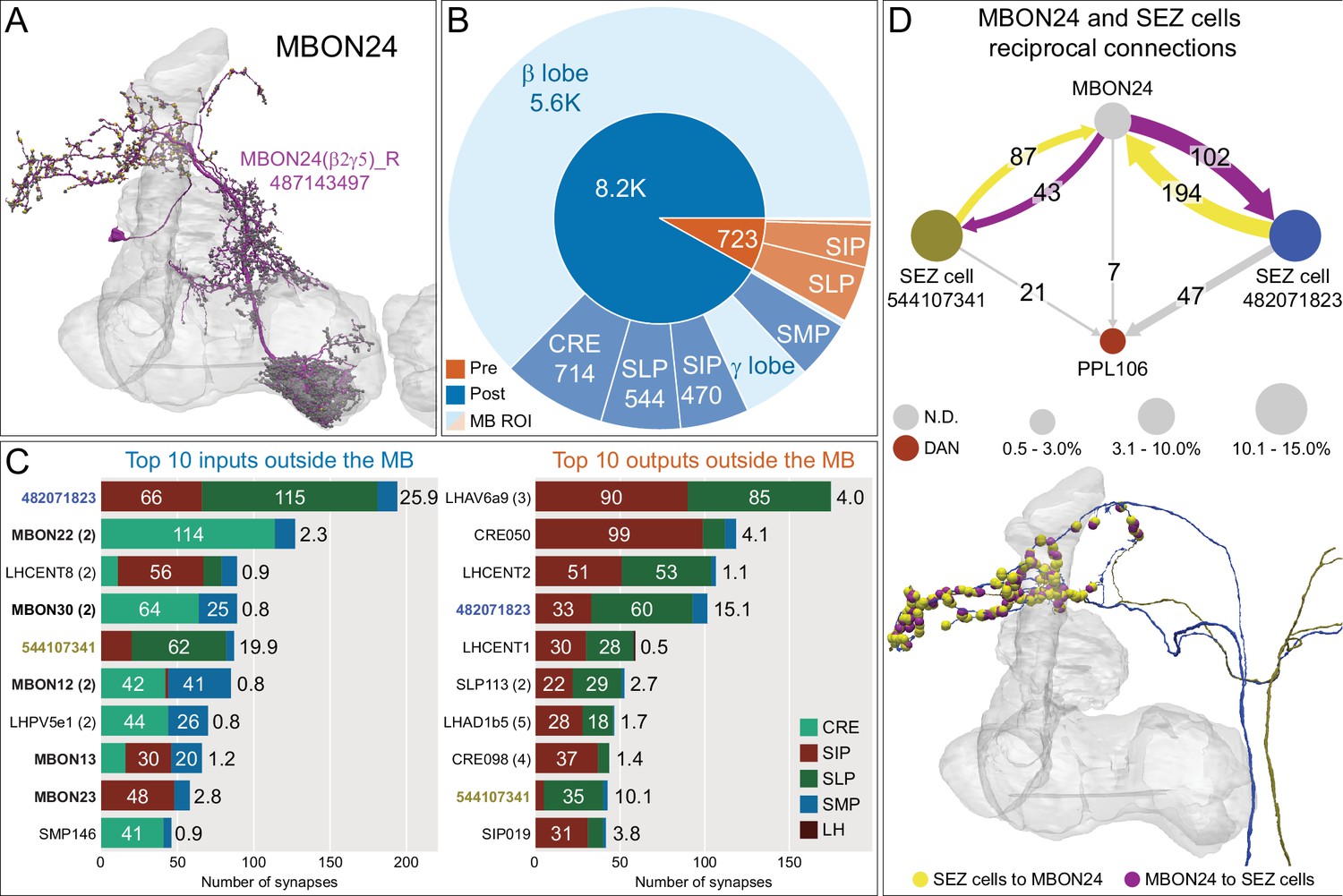
(A) Atypical MBON24 (β2γ5) is shown here and in Figure 8—video 3. Presynaptic sites are shown in yellow and postsynaptic sites are shown in gray. MBON24 receives 75% of its inputs from sites within the MB lobes and 90% of these inputs are in the β2 compartment. (B) A pie chart showing the distribution of MBON24’s presynaptic sites (indicated in orange) and postsynaptic sites (in blue). The inner circle shows the total number of MBON24’s pre- and postsynaptic sites. The outer circle of the pie chart shows the brain regions in which these sites occur; regions of the MB are shown in lighter colors. (C) MBON24’s top 10 inputs (left) and outputs (right) outside the MB lobes are shown by neuron type as bar charts. The numbers in each row represent synapse numbers and the brain regions in which these synapses occur are color-coded. (Left) T he numbers next to each row indicate the percentage of that neuron’s synaptic output that goes to MBON24. Links to these cell types in neuPrint are: 482071823, MBON22, LHCENT8, MBON30, 544107341, MBON12, LHPV5e1, MBON13, MBON23, and SMP146. Note that four of MBON24’s top input neurons are typical MBONs (indicated by bold text). (Right) T he numbers next to each row indicate the fraction of that neuron's input that is provided by MBON24. Links to these cell types in neuPrint are: LHAV6a9, CRE050, LHCENT2, 482071823, LHCENT1, SLP113, LHAD1b5, CRE098, 544107341, and SIP019. Neuron names in colored text indicate neurons further discussed in panel D and are color-coded to match the diagrams in panel D. (D) Two of the top inputs to MBON24, and MBON24’s reciprocal connections back to them, are shown. These cells send processes outside of the hemibrain volume, presumably to the subesophageal zone (SEZ), as has been confirmed for the more strongly connected of the two (482071823) by reconstructing its counterpart in the FAFB volume (Figure 35C,E). The same two neurons also provide strong input to a PPL106, contributing more than 0.5% of its total input, and are part of cluster 27 of DAN inputs shown in Figure 31. These SEZ cells also receive strong input from MBON14 (387 synapses). The size of the MBON24 circle indicates the percent of its total output (based on synapse number) that goes to PPL106 and SEZ neurons; while the sizes of the circles of the SEZ neurons and PPL106 reflect the percentage of that cell's input that comes from MBON24.
Figure 8—figure supplement 4

Atypical MBON25.
(A) Atypical MBON25 (γ1γ2) is shown here and in Figure 8—video 4. Presynaptic sites are shown in yellow and postsynaptic sites are shown in gray. MBON25 receives input in the γ1 and γ2 compartments. (B) A pie chart showing the distribution of MBON25’s presynaptic sites (indicated in orange) and postsynaptic sites (in blue). The inner circle shows the total number of MBON25’s pre- and postsynaptic sites. The outer circle of the pie chart shows the brain regions in which these sites occur; regions of the MB are shown in lighter colors. The CRE is MBON25’s major output area and MBON25 extends bilaterally to the left hemisphere CRE. (C) MBON25’s top 10 inputs (left) and outputs (right) outside the MB lobes are shown by neuron type as bar charts. The numbers in each row represent synapse numbers and the brain regions in which these synapses occur are color-coded. (Left) T he numbers next to each row indicate the percentage of that neuron’s synaptic output that goes to MBON25. Links to these cell types in neuPrint are: AVLP563, CRE029_a, SMP593, CL303, SMP026, CRE033, PLP161, AVLP473, 925811326, and PPL101. (Right) T he numbers next to each row indicate the fraction of that neurons input that is provided by MBON25. Links to these cell types in neuPrint are: PPL108, AVLP563, MBON20, CRE043_c, AstA1, PAM07, 1453176009, CRELALFB4_4 (FB4H), CRE027, and CRENO2,3FB1-4 (FB1H). MBON25 makes axo-dendritc connections outside the MB onto MBON20 (light orange shading); MBON20 and MBON25 both innervate the γ1 and γ2 compartments.
Figure 8—figure supplement 5

Atypical MBON26.
(A) Atypical MBON26 (β′2d) is shown here and in Figure 8—video 5. Presynaptic sites are shown in yellow and postsynaptic sites are shown in gray. MBON26 receives input from the β′2 compartment. (B) A pie chart showing the distribution of MBON26’s presynaptic sites (indicated in orange) and postsynaptic sites (in blue). The inner circle shows the total number of MBON26’s pre- and postsynaptic sites. The outer circle of the pie chart shows the brain regions in which these sites occur; regions of the MB are shown in lighter colors. Note MBON26_R’s output in LAL(L) is incomplete due to the left LAL(L) being only partially contained within the hemibrain volume (see panel D); to display in the output pie chart what we believe to be MBON26’s full output in both LALs we combined the output of MBON26_L in LAL(R) with that of MBON26_R in LAL(R). (C) MBON26’s top 10 inputs (left) and outputs (right) outside the MB lobes are shown by neuron type as bar charts. The numbers in each row represent synapse numbers and the brain regions in which these synapses occur are color-coded. (Left) The numbers next to each row indicate the percentage of that neuron’s synaptic output that goes to MBON26. Links to these cell types in neuPrint are: MBON32, MBON31, MBON21, MBON30, LAL075, 5813023296, LAL051, CL021, SMP146, and ATL009. (Right) T he numbers next to each row indicate the fraction of that neurons input that is provided by MBON26. Links to these cell types in neuPrint are: LAL051, LAL171, 1822686129, LAL172, LAL115, IB048, LAL174, LAL135, LAL173, and LAL039. Note that MBON26’s strongest inputs come from MBON21 (γ4γ5) and three atypical MBONs, MBON30 (γ1γ2γ3), MBON31 (α′1) and MBON32 (γ2). MBON26 is at the top layer of an MBON feedforward hierarchy network and also gets strong input from MBON27 (γ5d) and MBON29 (γ4γ5) (Figure 24). (D,E) The connections from MBON31 and MBON32 to MBON26 occur almost exclusively in the LAL.
Figure 8—figure supplement 6
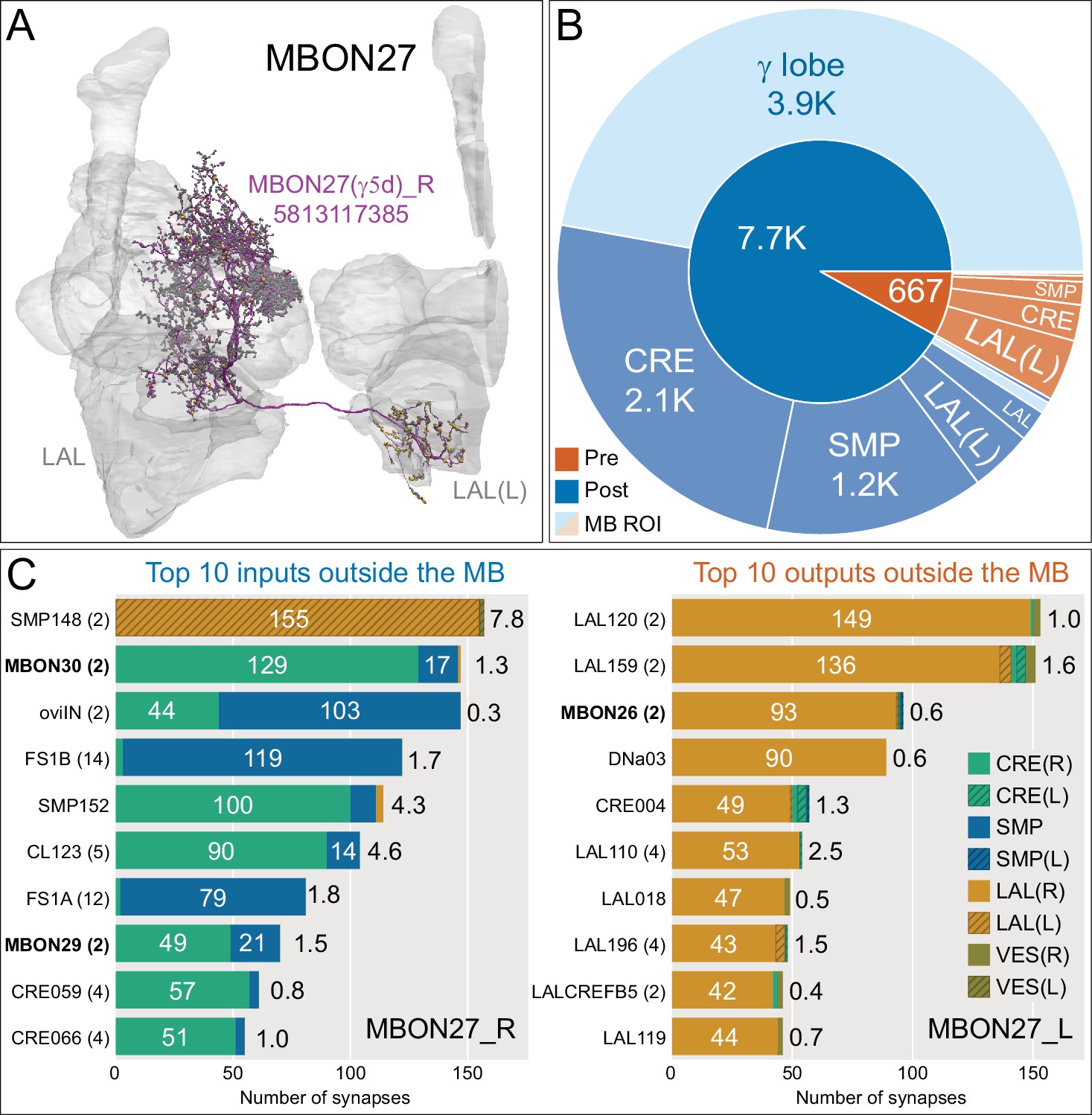
Atypical MBON27.
(A) Atypical MBON27 (γ5d) is shown here and in Figure 8—video 6. Presynaptic sites are shown in yellow and postsynaptic sites are shown in gray. MBON27 receives about half its input inside the MB, from the γ5 compartment, and outputs to both the ipsi- and contralateral LALs. (B) A pie chart showing the distribution of MBON27’s presynaptic sites (indicated in orange) and postsynaptic sites (in blue). The inner circle shows the total number of MBON27’s pre- and postsynaptic sites. The outer circle of the pie chart shows the brain regions in which these sites occur; regions of the MB are shown in lighter colors. The LAL is MBON27’s major output area. (C) MBON27’s top 10 inputs (left) and outputs (right) outside the MB lobes are shown by neuron type as bar charts. The numbers in each row represent synapse numbers and the brain regions in which these synapses occur are color-coded. (Left) T he numbers next to each row indicate the percentage of that neuron’s synaptic output that goes to MBON27. Links to these cell types in neuPrint are: SMP148, MBON30, oviIN, FS1B, SMP152, CL123, FS1A, MBON29, CRE059, and CRE066. (Right) the numbers next to each row indicate the fraction of that neurons input that is provided by MBON27. Links to these cell types in neuPrint are: LAL120, LAL159, MBON26, DNa03, CRE004, LAL110, LAL018, LAL196, LALCREFB5 (FB5A), and LAL119. Note that MBON27 receives input from two atypical MBONs, MBON29 (γ4γ5), and MBON30 (γ1γ2γ3), and outputs onto another atypical MBON, MBON26 (β′2d).
Figure 8—figure supplement 7
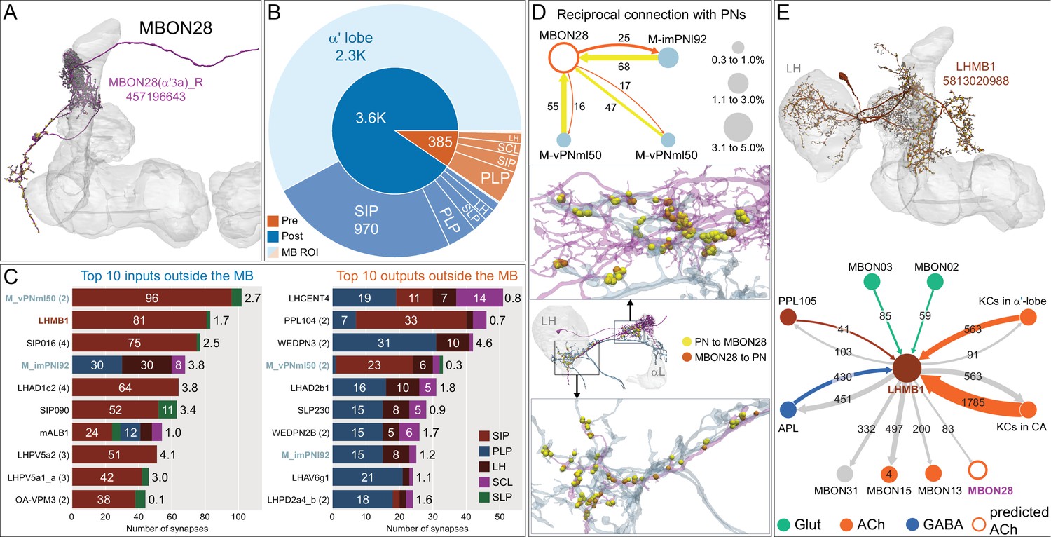
Atypical MBON28.
(A) Atypical MBON28 (α′3) is shown here and in Figure 8—video 7. Presynaptic sites are shown in yellow and postsynaptic sites are shown in gray. MBON28 receives about 60% of its input from the α′3 compartment within the MB lobes; within the α′3 compartment its arbors have a similar morphology to those of MBON16, but MBON28’s dendrites also extend outside the MB lobe. (B) A pie chart showing the distribution of MBON28’s presynaptic sites (indicated in orange) and postsynaptic sites (in blue). The inner circle shows the total number of MBON28’s pre- and postsynaptic sites. The outer circle of the pie chart shows the brain regions in which these sites occur; regions of the MB are shown in lighter colors. (C) MBON28’s top 10 inputs (left) and outputs (right) outside the MB lobes are shown by neuron type as bar charts. The numbers in each row represent synapse numbers and the brain regions in which these synapses occur are color-coded. (Left) T he numbers next to each row indicate the percentage of that neuron’s synaptic output that goes to MBON28. Links to these cell types in neuPrint are: M_vPNml50, LHMB1, SIP016, M_imPNl92, LHAD1c2, SIP090, mALB1, LHPV5a2, LHPV5a1_a, and OA-VPM3. (Right) T he numbers next to each row indicate the fraction of that neurons input that is provided by MBON28. Links to these cell types in neuPrint are: LHCENT4, PPL104, WEDPN3, M_vPNml50, LHAD2b1, SLP230, WEDPN2B, M_imPNl92, LHAV6g1, and LHPD2a4_b. Neurons with names in bold text are color-coded to match the diagrams in panel D. (D) MBON28 makes strong reciprocal connections with three inhibitory multi-glomerular PNs. The size of the circle representing the PN indicates the percentage of that PN’s output that goes to MBON28. The size of the MBON28 circle represents the percentage of its inputs outside the MB provided by the three PNs. This is the only MBON that receives PN input among its top 10 inputs. These reciprocal connections are distributed in two major areas: one near the MB, the other near or inside the LH. (E) Top: MBON28’s second strongest input neuron, LHMB1, is shown here and in Figure 8—video 7; LHMB1 innervates both the LH, the CA and the α lobe. Bottom: Connectivity diagram showing LHMB1’s main outputs and inputs. LHMB1 makes synapses onto MBONs on their dendrites inside the lobes as well as outside the MB through axo-axonal connections, and receives input from MBON02 (β2β′2a) and MBON03 (β′2mp), and reciprocally connects to APL and KCs in both the α lobe and CA.
Figure 8—figure supplement 8

Atypical MBON29.
(A) Atypical MBON29 (γ4γ5) is shown here and in Figure 8—video 8. Presynaptic sites are shown in yellow and postsynaptic sites are shown in gray. MBON29 receives about 80% of its input from the γ4 and γ5 compartments within the MB lobes. (B) A pie chart showing the distribution of MBON29’s presynaptic sites (indicated in orange) and postsynaptic sites (in blue). The inner circle shows the total number of MBON29’s pre- and postsynaptic sites. The outer circle of the pie chart shows the brain regions in which these sites occur; regions of the MB are shown in lighter colors. (C) MBON29’s top 10 inputs (left) and outputs (right) outside the MB lobes are shown by neuron type as bar charts. The numbers in each row represent synapse numbers and the brain regions in which these synapses occur are color-coded. (Left) T he numbers next to each row indicate the percentage of that neuron’s synaptic output that goes to MBON29. Links to these cell types in neuPrint are: MBON11, 582372162, CRE027, LHPV7c1, MBON30, SMP165, PAM08_b, SMP116, SMP384, and 612095452 (Right) T he numbers next to each row indicate the fraction of that neuron's input that is provided by MBON29. Links to these cell types in neuPrint are: MBON04, CRE080, PPL101, SMP076, SMP376, CRE050, MBON26, SMP120, CRE072, and MBON27. (Note that to ensure completeness of the contralateral arbor, MBON29_L was used.) Note that MBON29 receives very strong input from MBON11 (γ1pedc>α/β)_R and _L, which together contribute 9% of MBON29’s total input outside the MB. MBON28 also receives input from MBON30 (γ1γ2γ3). MBON29 makes axo-axonal synapses onto MBON04 (β′2mp_bilateral) as well as onto atypical MBONs, MBON26 (β′2d), and MBON27 (γ5d).
Figure 8—figure supplement 9
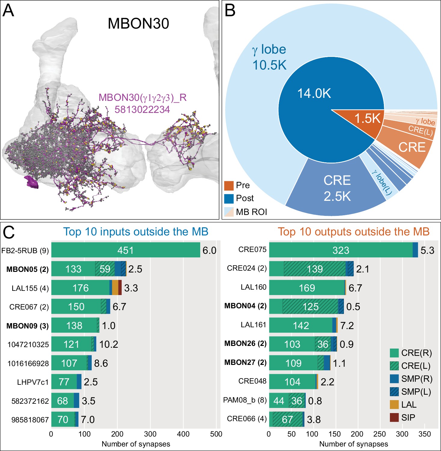
Atypical MBON30.
(A) Atypical MBON30 (γ1γ2γ3) is shown here and in Figure 8—video 9. Presynaptic sites are shown in yellow and postsynaptic sites are shown in gray. MBON30 receives about 80% of its input within the MB lobes, primarily from the γ1, γ2, and γ3 compartments. (B) A pie chart showing the distribution of MBON30’s presynaptic sites (indicated in orange) and postsynaptic sites (in blue). The inner circle shows the total number of MBON30’s pre- and postsynaptic sites. The outer circle of the pie chart shows the brain regions in which these sites occur; regions of the MB are shown in lighter colors. The CRE is MBON30’s major output area. (C) MBON30’s top 10 inputs (left) and outputs (right) outside the MB lobes are shown by neuron type as bar charts. The numbers in each row represent synapse numbers and the brain regions in which these synapses occur are color-coded. (Left) T he numbers next to each row indicate the percentage of that neuron’s synaptic output that goes to MBON30. Links to these cell types in neuPrint are: FR1, MBON05, LAL155, CRE067, MBON09, 1047210325, 1016166928, LHPV7c1, 582372162, and 985818067. MBON30 gets strong input from nine fan-shaped body cells of cell type FB2-5RUB (FR1; collectively they make 451 synapses onto MBON30’s arbors in a small brain area called the rubus (see Figure 8—video 9)). (Right) The numbers next to each row indicate the fraction of that neurons input that is provided by MBON30. Links to these cell types in neuPrint are: CRE075, CRE024, LAL160, MBON04, LAL161, MBON26, MBON27, CRE048, PAM08_b, and CRE066. Note that MBON30 receives input from MBON05 (γ4>γ1γ2) and MBON09 (γ3β′1) and makes synapses onto the atypical MBONs MBON27 (γ5d) and MBON28 (α′3) as well as to typical MBON04 (β′2mp_bilateral).
Figure 8—figure supplement 10
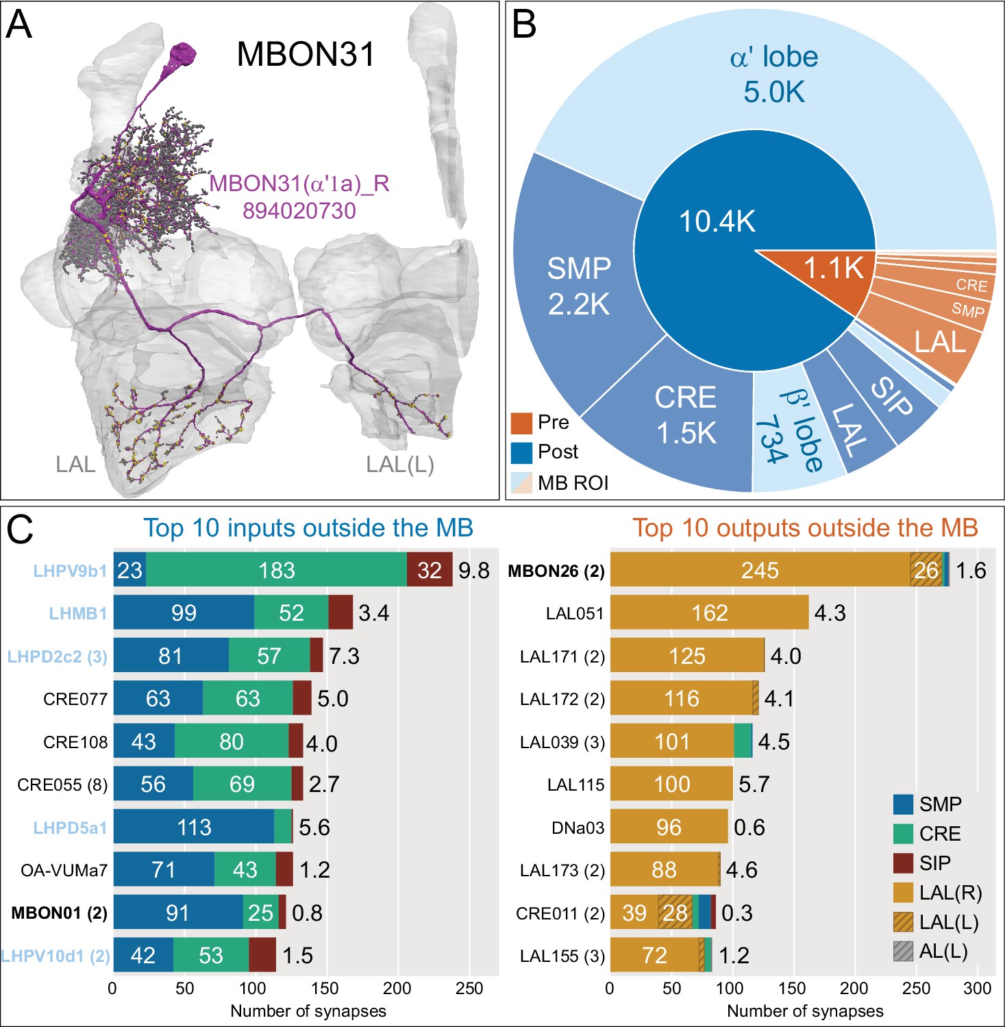
Atypical MBON31.
(A) Atypical MBON31 (α′1a) is shown here and in Figure 8—video 10. Presynaptic sites are shown in yellow and postsynaptic sites are shown in gray. MBON31 gets about half of its inputs from the α′1 compartment inside the MB and sends outputs to LAL. (B) A pie chart showing the distribution of MBON31’s presynaptic sites (indicated in orange) and postsynaptic sites (in blue). The inner circle shows the total number of MBON31’s pre- and postsynaptic sites. The outer circle of the pie chart shows the brain regions in which these sites occur; regions of the MB are shown in lighter colors. (C) MBON31’s top 10 inputs (left) and outputs (right) outside the MB lobes are shown by neuron type as bar charts. The numbers in each row represent synapse numbers and the brain regions in which these synapses occur are color-coded. (Left) T he numbers next to each row indicate the percentage of that neuron’s synaptic output that goes to MBON31. Links to these cell types in neuPrint are: LHPV9b1, LHMB1, LHPD2c2, CRE077, CRE108, CRE055, LHPD5a1, OA-VUMa7, MBON01, and LHPV10d1. (Right) The numbers next to each row indicate the fraction of that neurons input that is provided by MBON31. Links to these cell types in neuPrint are: MBON26, LAL051, LAL171, LAL172, LAL039, LAL115, DNa03, LAL173, CRE011, and LAL155. MBON31 top 10 inputs include five cell types that convey information from the LH and MBON01 (γ5β'2a); its strongest downstream target is the atypical MBON, MBON26 (β′2d).
Figure 8—figure supplement 11
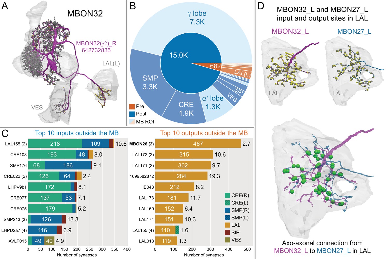
Atypical MBON32.
(A) Atypical MBON32 (γ2) is shown here and in Figure 8—video 11. Presynaptic sites are shown in yellow and postsynaptic sites are shown in gray. MBON32 gets about 50% of its synaptic input inside the MB lobes, primarily from the γ2 compartment, and sends about half its output to the contralateral LAL. (B) A pie chart showing the distribution of MBON32’s presynaptic sites (indicated in orange) and postsynaptic sites (in blue). The inner circle shows the total number of MBON32’s pre- and postsynaptic sites. The outer circle of the pie chart shows the brain regions in which these sites occur; regions of the MB are shown in lighter colors. (C) MBON32’s top 10 inputs (left) and outputs (right) outside the MB lobes are shown by neuron type as bar charts. The numbers in each row represent synapse numbers and the brain regions in which these synapses occur are color-coded. (Left) T he numbers next to each row indicate the percentage of that neuron’s synaptic output that goes to MBON32. Links to these cell types in neuPrint are: LAL155, CRE108, SMP176, CRE022, LHPV9b1, CRE077, CRE075, SMP213, LHPD2a7, and AVLP015. MBON32’s axon targets the contralateral LAL and the left brain hemisphere is incomplete in the hemibrain volume; therefore, we used MBON32_L’s arbors in the right hemisphere to ascertain MBON32’s downstream targets. (Right) T he numbers next to each row indicate the fraction of that neuron's input that is provided by MBON32. Links to these cell types in neuPrint are: MBON26, LAL172, LAL171, 1699582872, IB048, LAL173, LAL169, LAL174, LAL155, and LAL018. (D) We use the MBON32_L to illustrate MBON32’s downstream targets in the right hemisphere LAL. MBON27 (γ5d)’s axon also targets contralateral LAL (see Figure 8—figure supplement 6); the arbors of MBON32 and MBON27 in the LAL are shown separately in the upper portion of panel (D) with their pre- (yellow) and postsynaptic (gray) sites indicated. MBON32_L makes axo-axonal synapses onto MBON27_L, indicated by the green dots (lower portion of panel (D)).
Figure 8—figure supplement 12
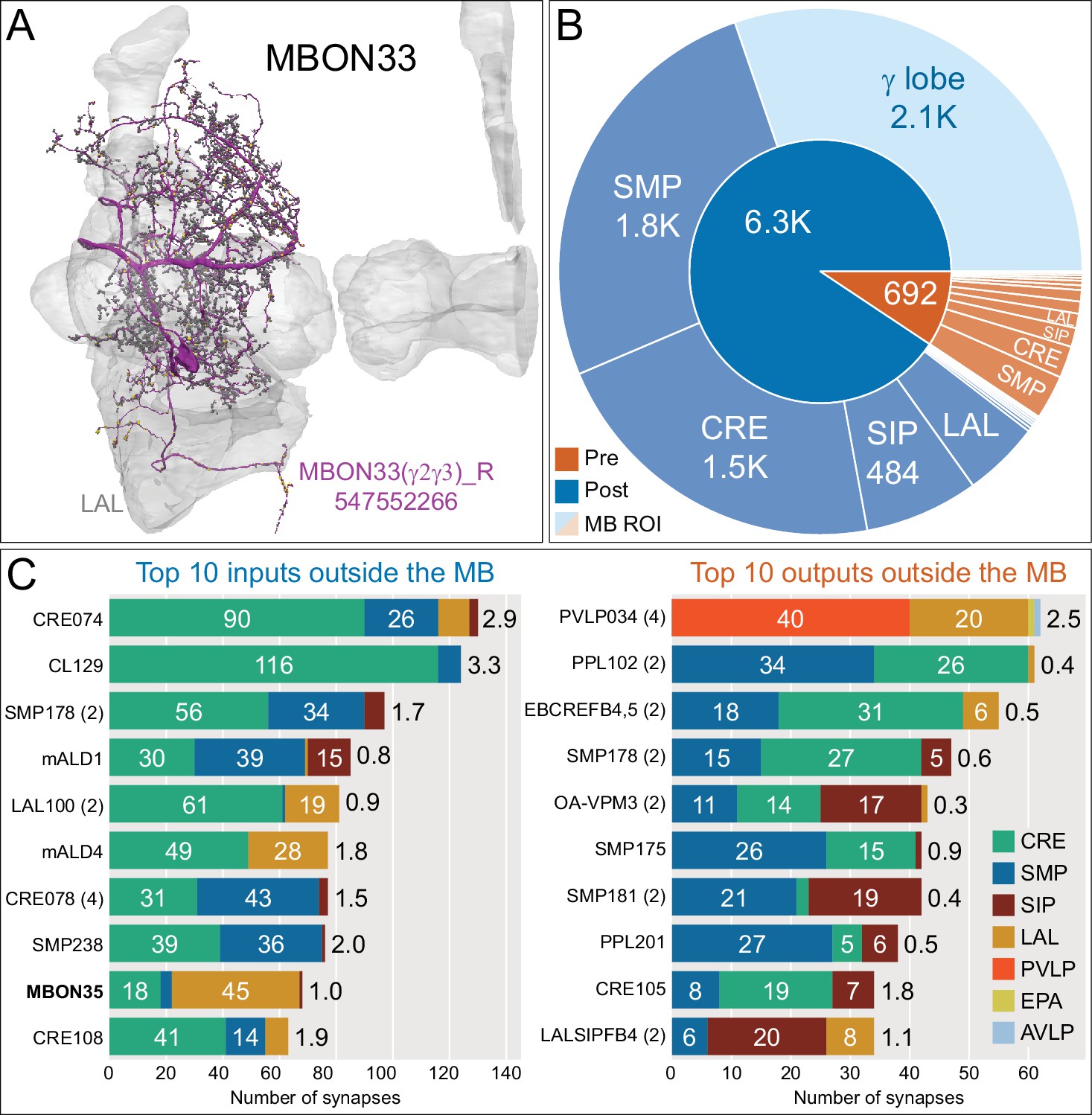
Atypical MBON33.
(A) Atypical MBON33 (γ2γ3) is shown here and in Figure 8—video 12. Presynaptic sites are shown in yellow and postsynaptic sites are shown in gray. MBON33 gets about one-third of its input synapses within the γ lobe of the MB, mostly in the γ2 and γ3 compartments, and sends about 9% of its output to the LAL. (B) A pie chart showing the distribution of MBON33’s presynaptic sites (indicated in orange) and postsynaptic sites (in blue). The inner circle shows the total number of MBON33’s pre- and postsynaptic sites. The outer circle of the pie chart shows the brain regions in which these sites occur; regions of the MB are shown in lighter colors. (C) MBON33’s top 10 inputs (left) and outputs (right) outside the MB lobes are shown by neuron type as bar charts. The numbers in each row represent synapse numbers and the brain regions in which these synapses occur are color-coded. (Left) T he numbers next to each row indicate the percentage of that neuron’s synaptic output that goes to MBON33. Links to these cell types in neuPrint are: CRE074, CL129, SMP178, mALD1, LAL100, mALD4, CRE078, SMP238, MBON35, and CRE108. (Right) T he numbers next to each row indicate the fraction of that neurons input that is provided by MBON33. Links to these cell types in neuPrint are: PVLP034, PPL102, EBCREFB4,5 (FB4Y), SMP178, OA-VPM3, SMP175, SMP181, PPL201, CRE105, and LALSIPFB4 (FB4L).
Figure 8—figure supplement 13
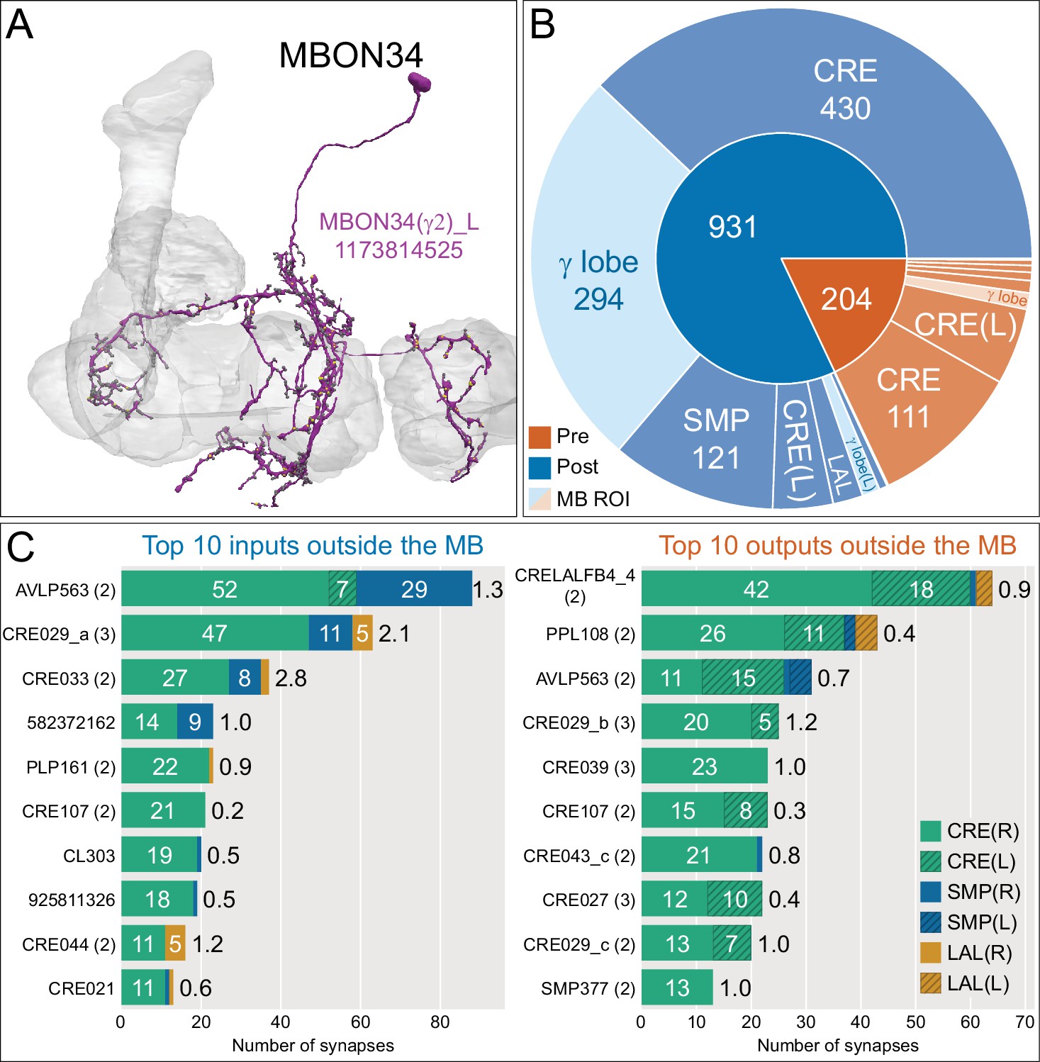
Atypical MBON34.
(A) Atypical MBON34 (γ2) is shown here and in Figure 8—video 13. Presynaptic sites are shown in yellow and postsynaptic sites are shown in gray. MBON34 has a small arbor and gets about one-third of its synapses from the γ2 compartment inside the MB lobes. (B) A pie chart showing the distribution of MBON34’s presynaptic sites (indicated in orange) and postsynaptic sites (in blue). The inner circle shows the total number of MBON34’s pre- and postsynaptic sites. The outer circle of the pie chart shows the brain regions in which these sites occur; regions of the MB are shown in lighter colors. (C) MBON34’s top 10 inputs (left) and outputs (right) outside the MB lobes are shown by neuron type as bar charts. The numbers in each row represent synapse numbers and the brain regions in which these synapses occur are color-coded. (Left) T he numbers next to each row indicate the percentage of that neuron’s synaptic output that goes to MBON34. Links to these cell types in neuPrint are: AVLP563, CRE029_a, CRE033, 582372162, PLP161, CRE107, CL303, 925811326, CRE044, and CRE021. (Right) T he numbers next to each row indicate the fraction of that neuron's input that is provided by MBON34. Links to these cell types in neuPrint are: CRELALFB4 _4 (FB4H), PPL108, AVLP563, CRE029_b, CRE039, CRE107, CRE043_c, CRE027, CRE029_c, and SMP377.
Figure 8—figure supplement 14
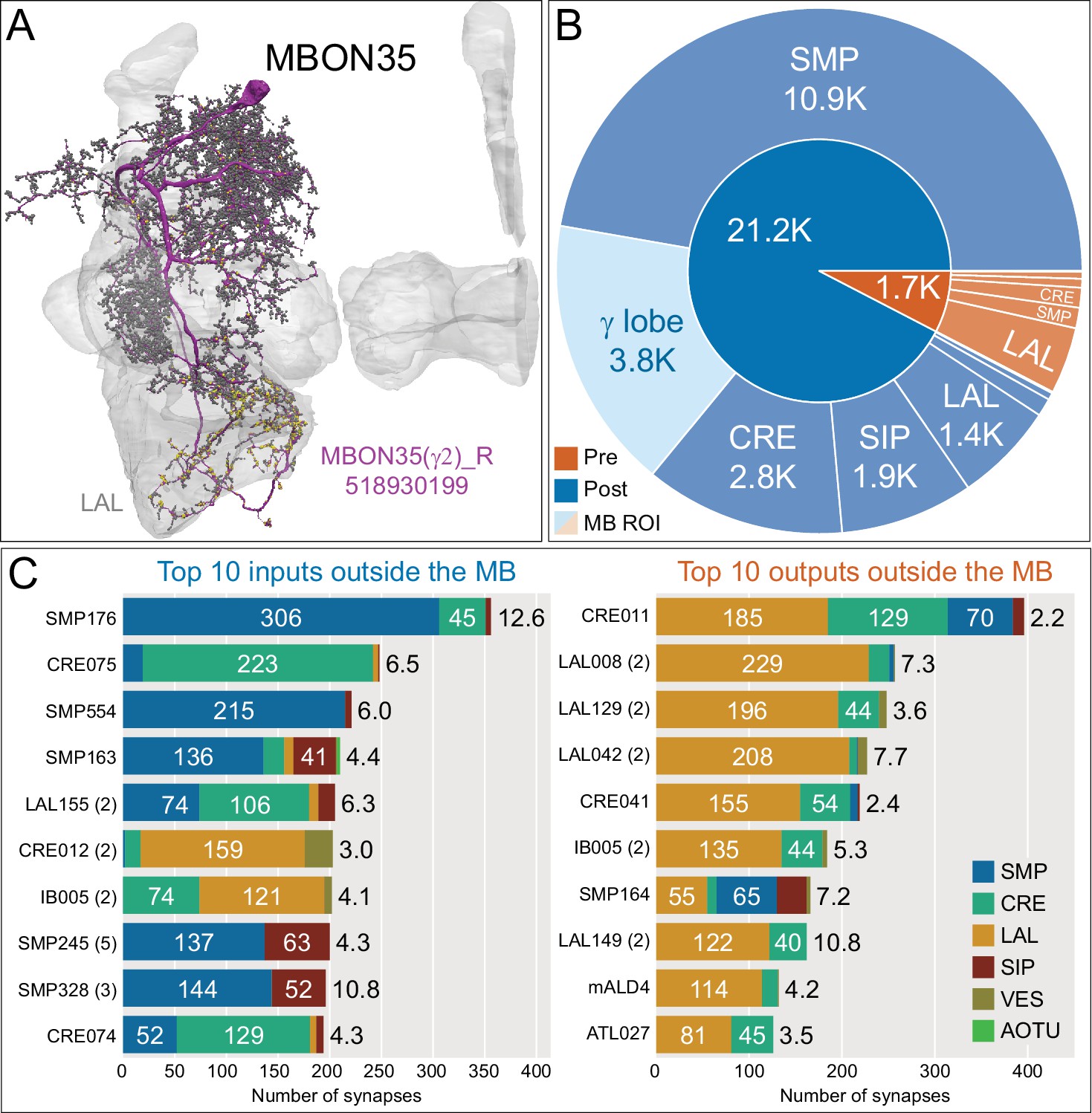
Atypical MBON35.
(A) Atypical MBON35 (γ2) is shown here and in Figure 8—video 14. Presynaptic sites are shown in yellow and postsynaptic sites are shown in gray. MBON35 gets about 20% of its input from the γ2 compartment inside the MB lobes and sends about half its output to the LAL. (B) A pie chart showing the distribution of MBON35’s presynaptic sites (indicated in orange) and postsynaptic sites (in blue). The inner circle shows the total number of MBON35’s pre- and postsynaptic sites. The outer circle of the pie chart shows the brain regions in which these sites occur; regions of the MB are shown in lighter colors. (C) MBON35’s top 10 inputs (left) and outputs (right) outside the MB lobes are shown by neuron type as bar charts. The numbers in each row represent synapse numbers and the brain regions in which these synapses occur are color-coded. (Left) The numbers next to each row indicate the percentage of that neuron’s synaptic output that goes to MBON35. Links to these cell types in neuPrint are: SMP176, CRE075, SMP554, SMP163, LAL155, CRE012, IB005, SMP245, SMP328, and CRE074. (Right) The numbers next to each row indicate the fraction of that neurons input that is provided by MBON35. Links to these cell types in neuPrint are: CRE011, LAL008, LAL129, LAL042, CRE041, IB005, SMP164, LAL149, mALD4, and ATL027.
Figure 8—figure supplement 15
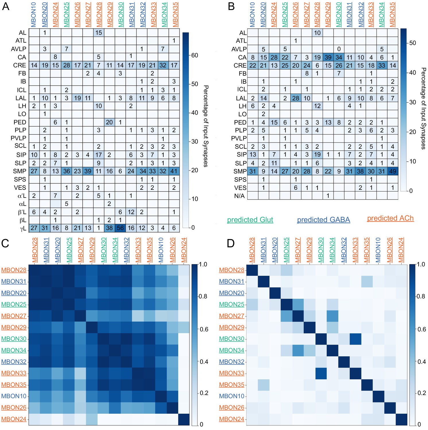
Atypical MBON input distribution by brain region and similarity of inputs to different MBONs.
(A–B) Distribution of brain regions providing input to atypical MBON types. The value in each box indicates the effective input to the indicated MBON from the indicated brain region; that is, based on where the neurons making synapses onto the MBONs get their own inputs. Effective input is a measure that takes into account both the strength of the connection of each of the neurons that provides input to the MBON and the connection strength of other neurons to each of those input neurons in each brain region. Effective input is computed by matrix-multiplying the inputs to the MBONs and the inputs to those MBON-presynaptic neurons (normalizing both matrices so that inputs to all neurons sum to 1). Blank boxes indicate values of less than 1%. Input received inside MB lobes is included in A and excluded in B. (C) Cosine similarity between MBON types based on their input at the level of brain regions, with the MB excluded. (D) Cosine similarity between each MBON based on their inputs, with the MB excluded and the computation of the degree of input overlap performed at the level of individual presynaptic neurons. The ordering of MBONs in C and D was determined using spectral clustering.
Figure 8—video 1
Atypical MBON10.
Figure 8—video 2
Atypical MBON20.
Figure 8—video 3
Atypical MBON24.
Figure 8—video 4
Atypical MBON25.
Figure 8—video 5
Atypical MBON26.
Figure 8—video 6
Atypical MBON27.
Figure 8—video 7
Atypical MBON28.
Figure 8—video 8
Atypical MBON29.
Figure 8—video 9
Atypical MBON30.
Figure 8—video 10
Atypical MBON31.
Figure 8—video 11
Atypical MBON32.
Figure 8—video 12
Atypical MBON33.
Figure 8—video 13
Atypical MBON34.
Figure 8—video 14
Atypical MBON35.
Figure 9 with 4 supplements
Main calyx (CA).
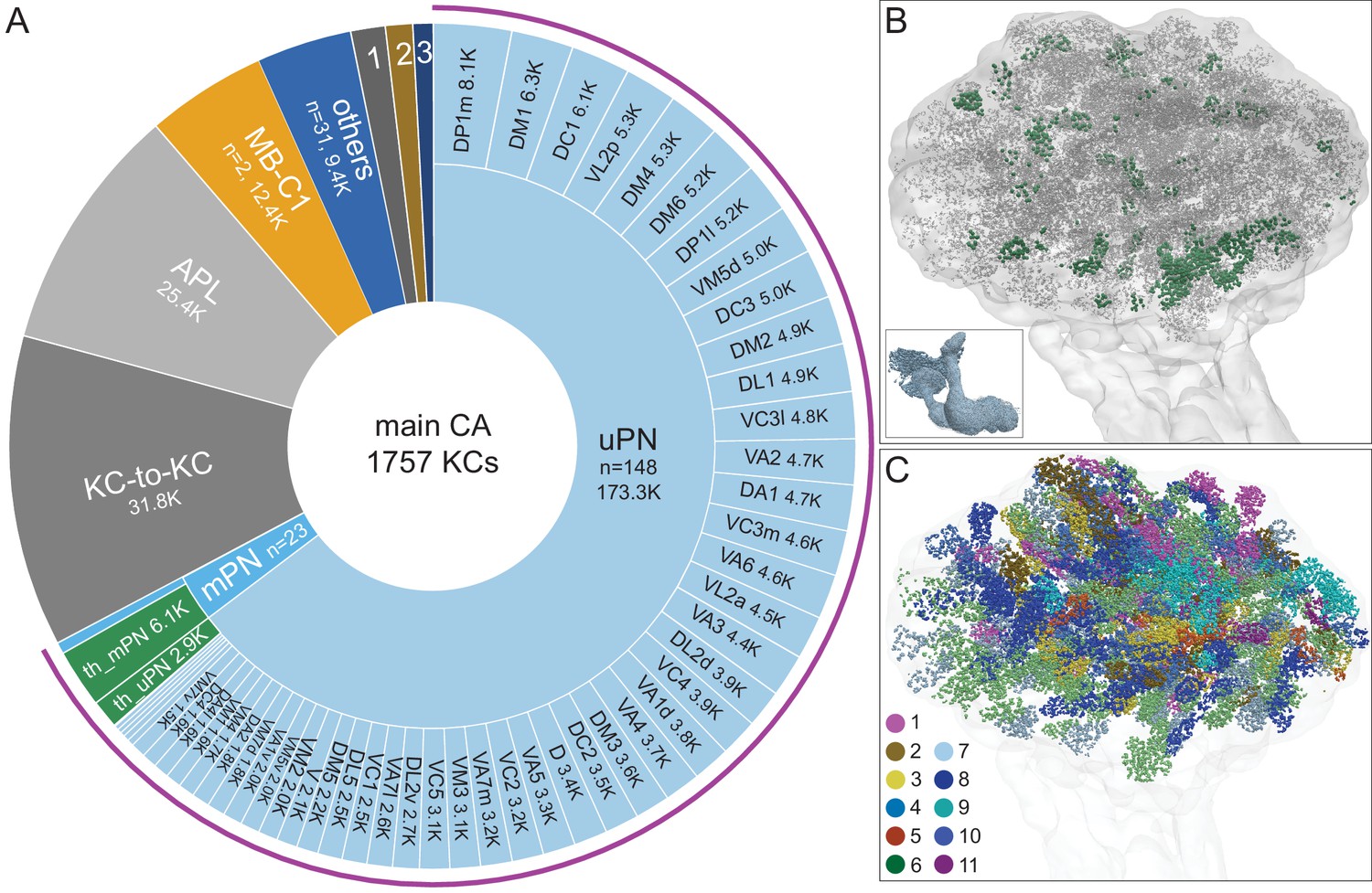
The dendrites of 1757 KCs of the α/β, α′/β′, and γ cell types define the CA. (A) The pie chart shows a breakdown of the inputs to these KCs. The largest source of input is from 129 uniglomerular olfactory projection neurons as judged by synapse number (uPNs; 63.6% of total input to the KCs); the number of synapses is indicated for each uPN cell type. Additional olfactory sensory input is provided by 23 multiglomerular projection neurons (mPNs). Information about temperature is provided by both 35 mPNs (th_mPN) and 19 uPNs (th_uPN). The next most prominent inputs are KC-to-KC synapses within the CA (11.9%), from APL (9.5%; see Figure 3—figure supplement 1A) and from MB-C1 (4.6%; see Figure 3—figure supplement 1H). Smaller sources of input are indicated by the numbered sectors: 1, a group of nine neurons previously described as ‘centrifugal’ neurons (Bates et al., 2020a) that innervate both CA and LH (1.3%). 2, MB-CP2 (1.0%); 3, PPL201 (see Figure 3—figure supplement 1G). The remaining 3.4% is provided by 31 other neurons (blue). (B) An image of the CA showing the locations of olfactory PN and thermo PN synapses onto KCs. The green dots representing thermo PN olfactory input synapses are of larger diameter to allow better visibility in the presence of the larger number of gray dots representing olfactory input synapses. Note the thermo PN inputs are located in the anterior and at the periphery of the CA, corresponding to the position of α′/β′ap1 and γt KC dendrites. The inset shows the orientation of the image. (C) Inputs from olfactory PNs are shown color-coded based on the type of olfactory information they are thought to convey (see Bates et al., 2020b): 1, fruity; 2, plant matter; 3, animal matter; 4, wasp pheromone; 5, insect alarm pheromone; 6, yeasty; 7, alcoholic fermentation; 8, decaying fruit; 9, pheromonal; 10, egg-laying related; 11, geosmin.
Figure 9—figure supplement 1

Distribution of the termini of olfactory PNs in the CA.
(A-A′′) MB images showing the orientation of the CA (blue) in panels B-E′′: (A) frontal view, (A′) top view, and (A′′) side view. (B-B′′) Four individual DL2d uniglomerular PNs (uPNs), each shown in a different color, innervate the CA, shown in faint gray. The axons of individual PNs split into two to three branches, each terminating in a large bouton that forms part of a highly stereotyped ‘claw-like’ connection with KCs (F; Figure 9—video 1). DL2d PNs terminate primarily in the anterior-lateral CA. (C-C′′) Synaptic connections, color-coded to correspond to the PNs in B-B′′, from DL2d PNs onto KCs. (D-D′′) DM1 and DC1 are shown; these uniglomerular PNs are unusual in that there is only a single cell of each type per brain hemisphere. Both DM1 and DC1 have widely distributed boutons, which occupy non-overlapping areas of the CA (Jeanne et al., 2018); DM1’s boutons are more dorsal and DC1’s more ventral. (E-E′′) Synaptic connections from the DM1 and DC1 PNs onto KCs, color-coded by PN type. (F) An example PN-to-KC synapse with a claw-like structure. DA1 lPN (1734350908; green) connects to KCγm (600356751; Figure 9—video 1; orange); note how the KC dendrite wraps around the PN bouton. Presynaptic sites of the PN and postsynaptic sites of the KC are shown in yellow and gray , respectively. (G–H) Distribution of the axons of DL2d, DM1 and DC1 in the LH and CA. (G) The four DL2d PNs innervate the middle of the LH. Note their axons terminate in the same area of the LH, but lack the large terminal boutons seen in the CA. (H) DM1 and DC1 axons remain segregated in the LH.
Figure 9—figure supplement 2
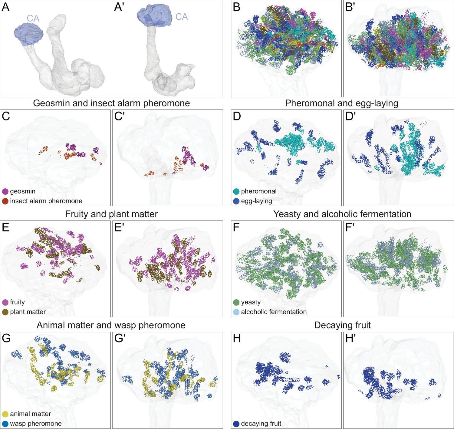
Spatial arrangement in the CA of synaptic input from different PN groups.
The synaptic terminals of PNs in the CA are shown. PNs that convey distinct types of olfactory information are shown separately as indicated. (A-A′) MB images indicating the orientation of the figures shown in remaining panels: (A) frontal view and (A′) top view. The CA is shaded blue. (B-B′). Synapses KCs receive from all the olfactory PN groups that are shown individually in panel C-H′. (C-C′) PNs that convey the presence of geosmin and insect alarm pheromone, both highly aversive odors, are clustered. (D-D′) PNs that convey pheromones and odors involved in egg-laying site selection occupy the center and periphery of the CA, respectively. (E-E′) PNs that convey fruity and plant matter information are distributed in the dorsal part of the CA. (F-F′) PNs that convey yeasty and alcoholic fermentation odors are distributed widely across the CA. (G-G′) PNs that convey wasp pheromone and animal matter information. (H, H′) PNs that convey decaying fruit information.
Figure 9—figure supplement 3
Gustatory input to a subset of KCs.
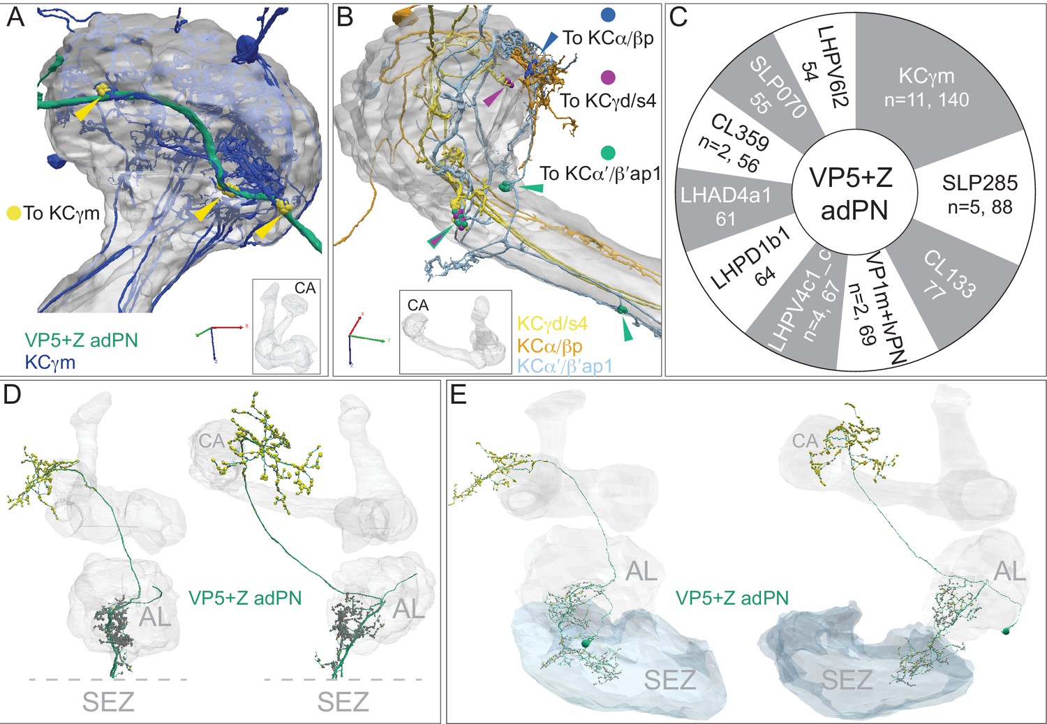
The PN, VP5+Z adPN, has been reported to receive sensory input with mixed modalities, with hygrosensory input from the VP5 glomerulus in the AL and gustatory input from the SEZ (Marin et al., 2020). We found that it connects to 16 KCs that extend a portion of their dendritic arbors outside the main CA. (A) Eleven γm KCs connect at three locations to the axon of VP5+Z adPN, just anterior to the main CA (indicated by yellow arrowheads), forming a total of 140 synapses. The same 11 γm KCs also have dendritic claws inside the CA (their dendrites are dark blue where they lie outside the CA and faint blue where they lie within the CA) where they receive input from many olfactory PN types; their synapses from VP5+Z adPN do not have a claw-like structure. VP5+Z adPN is the top PN input to these KCs. (B) Connections from VP5+Z adPN to other KC types are shown: three KCγd/s4 (purple, n = 30); two KCα/βp (blue, n = 13) and two KCα’/β’ap1 (green, n = 12). (C) Top 10 downstream targets of VP5+Z adPN by neuron type. Note that the 11 γm KCs are its top target. In addition to the neurons shown, two DNs are prominent downstream targets: DNp44 (542751938) with 52 synapses and DNg30 (571346836) with 33 synaspes. (D) VP5+Z adPN in the hemibrain (left: front view, right: side view) with presynaptic sites shown in yellow and postsynaptic sites in gray. Note the SEZ is not in the hemibrain volume and its putative position is indicated below the dashed lines, which mark the ventral extent of the hemibrain volume. (E) VP5+Z adPN traced in FAFB, with its complete dendrite in the SEZ where it receives strong input from gustatory receptor neurons (S. Engert and K. Scott, personal communication). The same two views as in panel D are shown; presynaptic (yellow) and postsynaptic (gray) sites are indicated.
Figure 9—video 1
Introduction to γ main KCs.
Figure 10 with 6 supplements
Ventral accessory calyx (vACA).
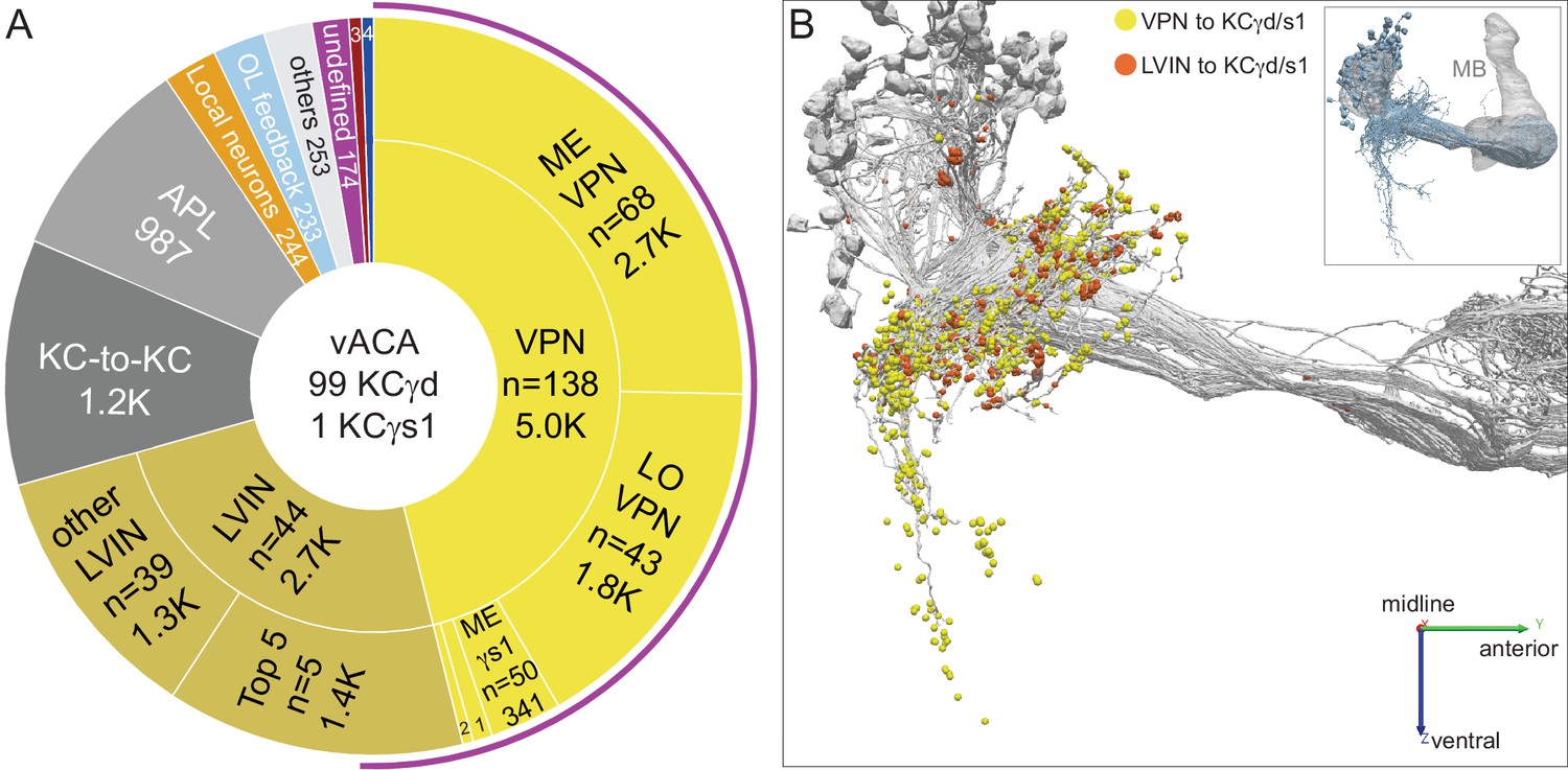
The dendrites of the 99 γd and one γs1 KCs define the vACA. (A) The pie chart shows a breakdown of the inputs to these KCs; the number of cell (n=) and the number of the total synapses contributed by the cells in that sector are shown without applying a threshold. The majority of inputs convey visual information, either directly from visual projection neurons (VPNs; 46.1%) or through intermediate local visual interneurons (LVIN; 24.6%) that themselves receive input from VPNs. The number of VPNs shown in the pie chart counts VPNs that make as few as one synapse. When a threshold is applied that requires a VPN to make at least five synapses to a single KC, then we find 49 VPNs, including 26 ME VPNs and 21 LO VPNs. The synapses from the VPNs and the LVINs onto the KCγd dendrites do not show the claw-like structure seen in the CA (Figure 10—video 1). A ranking of LVINs based on the amount of visual input conveyed is shown in Figure 10—figure supplement 2A. More than half of the indirect input is mediated by five LVINs (Top 5), which are shown in Figure 10—figure supplement 3B. VPNs can be subdivided based on the location of their dendrites in either the medulla (ME) or lobula (LO), as indicated in the outer circle. There are 68 VPNs that connect to the single KCγs1, with a total of 483 synapses: 50 from the ME, 34 of which are shared with other γd KCs, and 14 from the LO, eight of which are shared with other γd KCs (represented by the numbered sector 1). The next most prominent inputs to KCs in the vACA are synapses between the KCs themselves (10.8%), from APL (9.1%), from local interneurons that do not appear to convey significant visual information (2.3%), from interneurons that send feedback from the vACA to optic lobe neurons (OL feedback; 2.2%) and neurons that leave the volume with undefined identity (undefined; 1.6%). Other sources of input are indicated by the other numbered sectors: 2, other VPN input that we could not classify as from the ME or LO, due to incomplete morphology (0.9%); 3, three putative mPNs (0.6%) (5813063239, 1442819296, 5813040515); 4, three putative SEZ cells (0.5%). The remaining 2.3% is provided by 253 interneurons that are weakly connected to these KCs, with each providing one synapse to each of less than 4 KCs (others). The fraction of input to the vACA KCs conveying visual information is indicated by the outer purple arc; it reflects the direct input from the VPNs plus the fraction of the LVIN input that represents visual input. (B) Synaptic connections from visual projection neurons (VPN) and local visual interneurons (LVIN) onto γd and γs1 KCs (gray), color-coded. Note the different spatial distribution of synapses from VPNs and LVINs. VPNs make synapses onto KCγd dendrites in an area ventral to the CA, previously recognized as the vACA (Butcher et al., 2012), as well as in a diffuse ring surrounding the base of the CA; synapses from LVINs are restricted to the ring. Additional views are shown in Figure 10—figure supplement 4A, B.
Figure 10—figure supplement 1
Identification of VPNs.
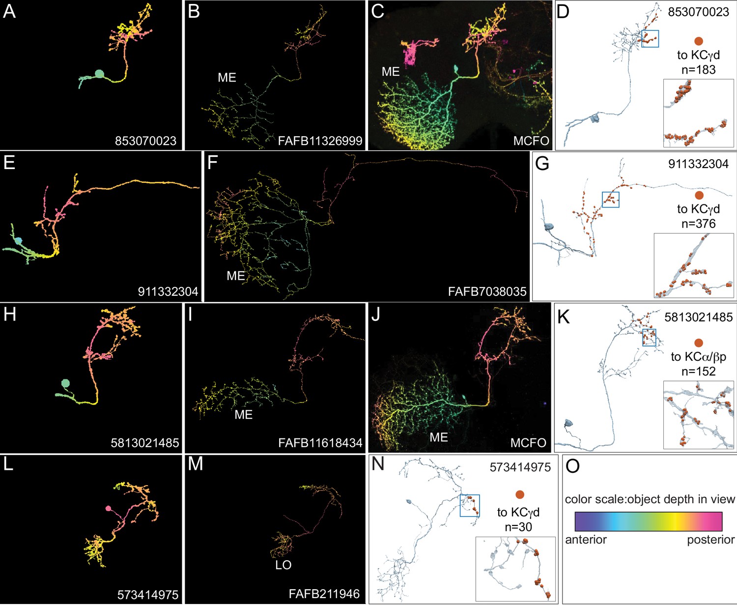
The arbors of the ME VPNs generally extend into portions of the optic lobes that are not contained in the hemibrain volume. In order to determine the locations in the optic lobes where their dendrites are located, we relied as much as possible on matching the portion of their neuronal arbors contained in the hemibrain with morphologies of complete neurons from two other datasets: neurons that we traced in FAFB (Zheng et al., 2018) or light microscopic images of single neurons derived using Multi-Color Flp-Out (Nern et al., 2015) of GAL4 lines. In other cases, we based our classification on the similarity of the morphology of the neuron to other VPNs and the position where its arbor left the hemibrain volume. This figure shows three examples of matching ME VPNs to their putative FAFB and MCFO counterparts (A–K) and one example showing an LO VPN that is totally contained within the hemibrain volume (L–N). The images shown in panels A-C, E,F, H-J and L,M are maximum intensity projections in which the color of the neuronal arbors reflects their anterior-posterior depth in the brain (see scale in panel O; Bailey and Clark, 1998; Ropinski et al., 2006; Otsuna et al., 2018). (A–C) An example of a ME VPN innervating the vACA from the hemibrain (A) and its likely equivalents in FAFB (B) and MCFO light data (C). (D) The reconstructed neuron from the hemibrain showing the positions on its axon of the 183 synapses that it makes onto a total of 20 γd KCs indicated by the orange dots; inset, enlarged view of the boxed area. (E–F) A second example of a vACA-innervating ME VPN from the hemibrain dataset (E) and its likely match in FAFB (F). (G) The reconstructed neuron from the hemibrain with the positions on its axon of the 376 synapses that it makes onto a total of 27 γd KCs and the single γs KC indicated by the orange dots; inset, enlarged view of the boxed area. (H–J) An example of a dACA-innervating ME VPN (H) and its likely matches in FAFB (I) and MCFO (J). (K) The reconstructed neuron from the hemibrain showing the positions on its axon of the 152 synapses it makes onto a total of 41 α/βp KCs; inset, enlarged view of the boxed area. (L–N) A vACA-innervating Lo VPN (L) and its likely matches in FAFB (M). Note how the entire arbor appears to be present in the hemibrain. (N) The reconstructed neuron from the hemibrain showing the positions on its axon of the 30 synapses that it makes onto a total of 2 γd KCs; inset, enlarged view of the boxed area. (O) Color-depth scale.
Figure 10—figure supplement 2

LVINs ranked by amount of visual information conveyed.
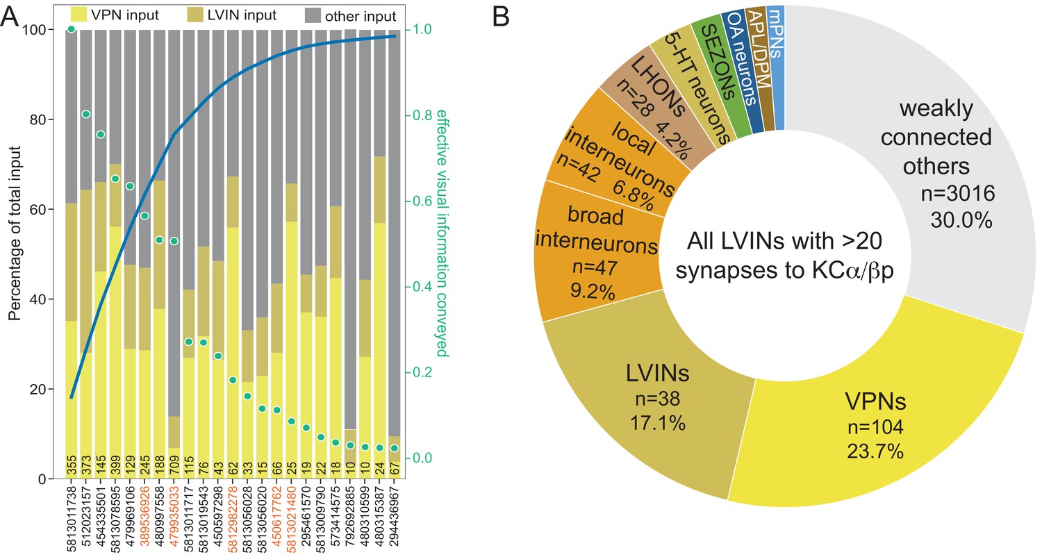
(A) Plot of interneurons carrying visual information to the γd and γs1 KCs ranked by the strength of their effective contribution of visual information. For a given interneuron, this quantity is computed by multiplying the number of synapses that interneuron makes onto γd and γs1 KCs by the fraction of its input synapses that come from visual projection neurons. The green dots show this effective visual information quantity. Values are normalized to the most strongly connected LVIN, which was assigned a value of 1.0 (green scale on the right side of the plot). The blue line shows the cumulative amount of effective visual information conveyed by LVINs; over 80% of the input is delivered by the top 10 LVINs. Links to these 10 LVINs in neuPrint are as follows: CL063, PLP095, PLP145, PLP120, CL258, SLP223 , CL200, and AVLP043. The color-coded bars indicate the percentage of that neuron’s input that comes from VPNs, other LVINs, and other neurons. The black number at the base of each bar shows the number of synapses made by that LVIN to KCs in the vACA. The LVINs whose ID numbers are shown in orange also provide input to the α/βp KCs in the dACA. Note that many of the lower ranked LVINs that receive high levels of VPN input do not make strong connections to KCs and are therefore presumably primarily performing some other role in integrating visual information. (B) Effective input delivered by the 15 LVINs that are the most strongly connected to the 99 γd and one γs1 KCs that are found in the vACA; each of these LVINs makes a total of 30 or more synapses to vACA KCs. Effective input is calculated by multiplying the indicated neuronal population’s synaptic input to each of the 15 LVINs times the fraction of the 99 γd and one γs1 KCs’ total input coming from that LVIN, and then summing across all 15 LVINs. Effective input is expressed as the percentage of the total input from these 15 LVINs to the 99 γd and one γs1 KCs that originated with the indicated neuronal population. To calculate the values presented, we considered the 408 neurons that collectively account for 70% of the total input synapses to these 15 LVINs and placed them into the categories shown in the pie chart; we did not attempt to classify the large number of diverse neurons (weakly connected others) that make up the other 30% of the input. VPNs, at 24.3%, provide the strongest category of effective input to vACA KCs mediated by LVINs. This visual input is in addition to direct input that VPNs make onto the dendrites of the KCs in the vACA; taking the direct and indirect pathways together, more than half the total input, and ~70% of the sensory input to the vACA is visual. We classified interneurons that did not receive visual input as local if their arbors were confined to the brain area around the vACA, as we observed for the LVINs, or broad, if they arborized in several brain areas. Although there is no direct input to γd or γs1 KCs from the SEZ, a group of 23 putative SEZONs contributes 3.6% of the LVINs effective input. Other inputs include OA-neurons (n = 5, 2.4%), LHONs (n = 21, 1.6%), 5-HT neurons (n = 4, 0.7%; numbered sector 1), and APL and DPM (0.6% combined; numbered sector 2).
Figure 10—figure supplement 3
Further description of LVINs upstream of vACA KCs.
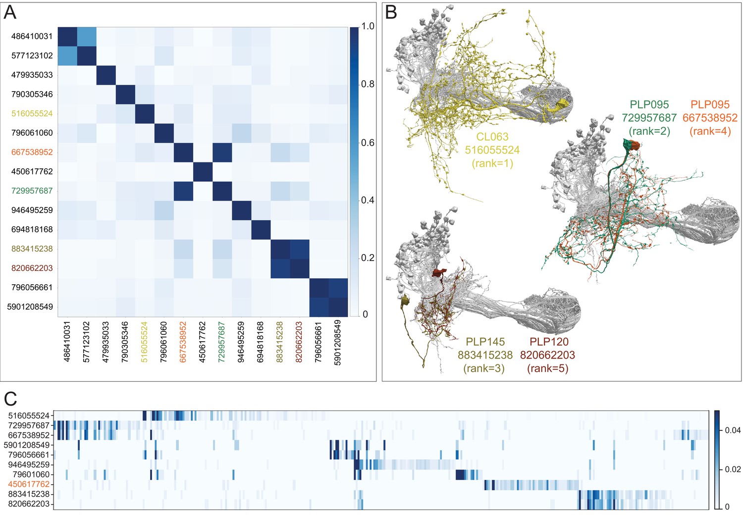
(A) A plot showing the similarity of the 15 LVINs most strongly connected to the vACA KCs, based on the cosine similarity of their inputs. The neuron IDs are color-coded to match the morphologies shown in (B). (B) The morphologies of the top five LVINs are shown; KCs are in gray. The orientation of the images is the same as in the inset shown in Figure 10B. (C) A plot showing the VPN inputs for each of the top 10 LVINs, using the ranking of effective visual input from Figure 10—figure supplement 2A. Each vertical blue bar represents a different VPN and the intensity of the color reflects the fraction of the corresponding LVIN’s total VPN input that is contributed by that VPN. The order of the VPNs and LVINs is determined using spectral clustering.
Figure 10—figure supplement 4

Additional views of the morphologies of VPN and LVIN inputs to the vACA.
(A–B) Additional views of the distribution of VPN and LVIN inputs onto γd and γs1 KCs (gray); synapses are color-coded as indicated. The insets show the orientation of the view shown. Note the spatial segregation of these two types of connections. VPNs onto KCγd dendrites in an area ventral to the CA, previously recognized as the vACA (Butcher et al., 2012), as well as in a diffuse ring surrounding the base of the CA; synapses from LVINs are restricted to the ring. An additional view is shown in Figure 10B. (C) The morphologies of the LVINs ranked sixth to tenth in conveying the highest visual input to the vACA are shown; KCs are in gray. The orientation of the images is the same as the inset shown in Figure 10B.
Figure 10—figure supplement 5
Distribution of VPN inputs onto an LVIN.
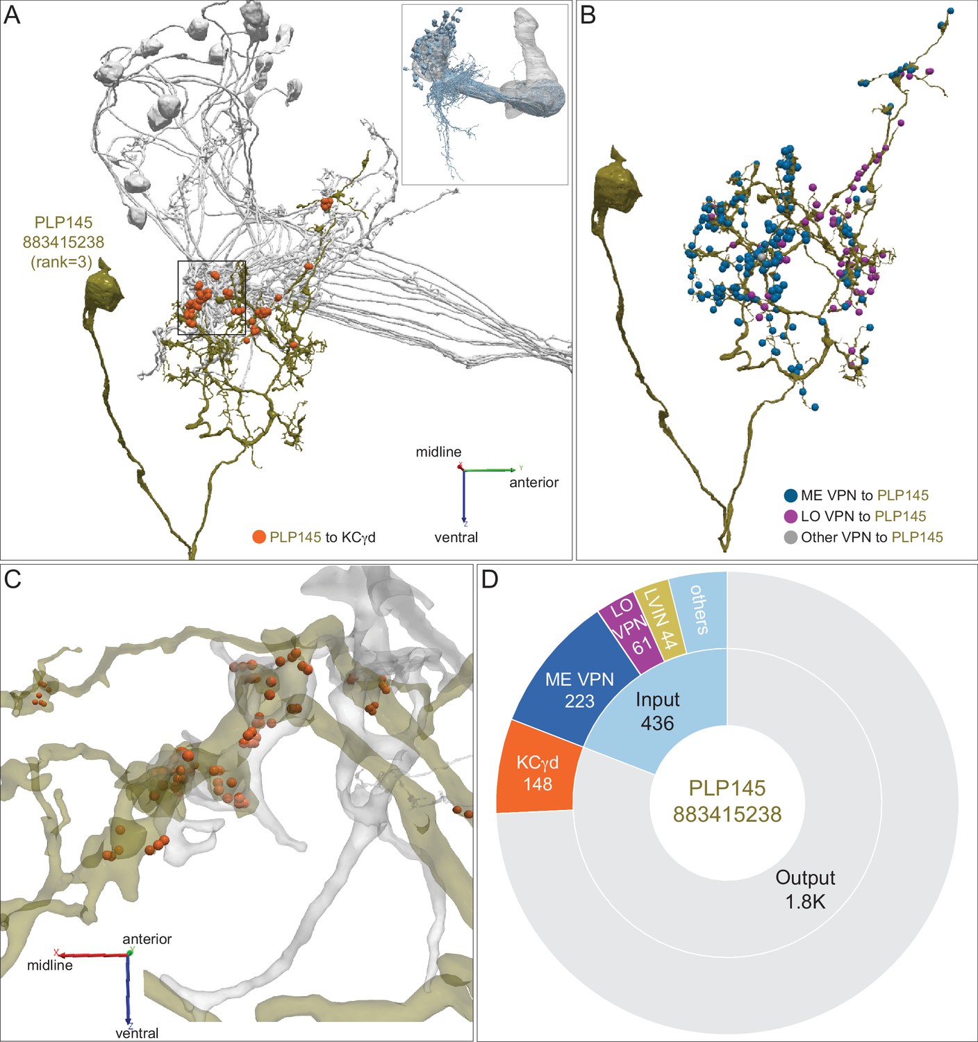
(A) The LVIN PLP145 (883415238; green) that conveys the third highest amount of visual input to the vACA is shown along with the positions where it makes synaptic output (orange dots) onto a subset of γd KCs (gray). The inset shows the orientation of the MB in this image. (B) PLP145 receives synaptic input from three classes of VPNs: ME, LO, others, shown color-coded. Some VPNs (others) could not be placed into the ME or LO groups based on their arbors in the hemibrain volume or that appear to have dendrites in both ME and LO. (C) Enlarged and rotated view of the boxed area in (A). Note that synaptic connections from PLP145 to γd KCs lack the claw-like structure typical of olfactory PN-to-KC connections in the CA. (D) Pie chart showing the portion of the total input to PLP145 (light blue) that comes from direct ME (dark blue) and LO VPNs (purple), other LVINs (yellow) and other neurons (blue); the portion of PLP145’s total output (gray) that goes to KCγd (orange) is also shown.
Figure 10—video 1
Introduction to γ dorsal KCs.
Figure 11 with 5 supplements
Dorsal accessory calyx (dACA).
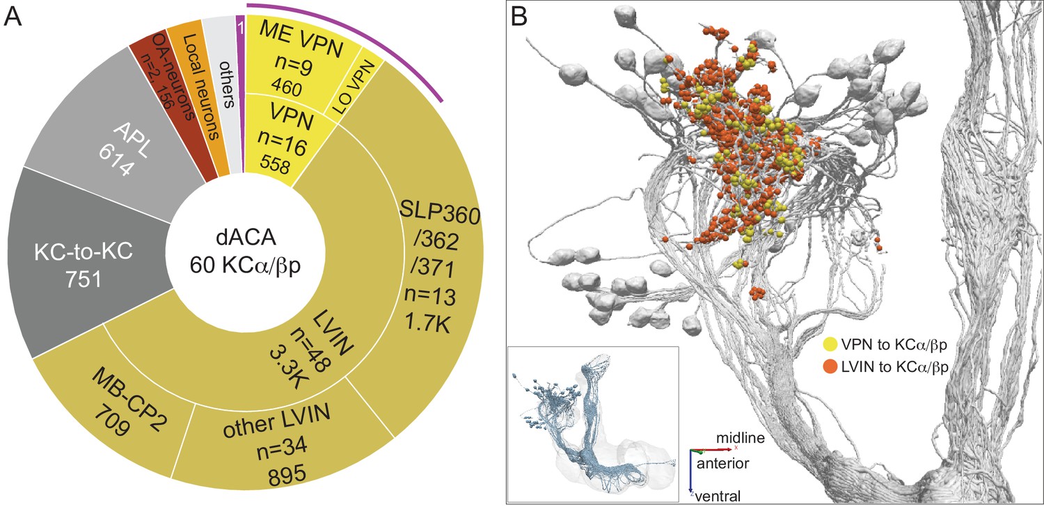
The dendrites of the 60 α/βp KCs define the dACA. The pie chart shows a breakdown of the inputs to these KCs. The majority convey visual information, either directly from visual projection neurons (VPN; 9.8%) or through intermediate local visual interneurons (LVIN; 57.8%) that receive input from VPNs (see Figure 11—figure supplement 1). VPNs can be subdivided based on the location of their dendrites in either ME or LO, as indicated in the outer circle. More than two-thirds of the indirect input is mediated by the LVIN cell types SLP360, SLP362, and SLP371, shown in Figure 11—figure supplement 2C; this SLP360/361/371 cluster of 13 neurons contributes about 30% of total input to the 60 α/βp KCs in the dACA. Neurons of similar morphology have also been observed to be presynaptic to KCα/βp in the dACA in a recent study (Li et al., 2020). Another LVIN, MB-CP2 (LHPV3c1) (479935033), provides 12.6% of the input to KCs in the dACA; however, only a small percentage of its inputs are visual (see Figure 11—figure supplement 1A and 2E). The total visual information presented to KCs by VPNs and LVINs is indicated by the purple arc around the outer layer; it reflects the direct input from the VPNs plus the fraction of the LVIN input that represents visual input. The next most prominent inputs are KC-to-KC synapses in the dACA (13.3%), from APL (10.9%), from two octopaminergic neurons (2.8%; OA-VPM3, see Figure 3—figure supplement 1D, and OA-VUMa2, see Figure 3—figure supplement 1F); and local interneurons (n = 23; 2.3%). Remaining input, ‘others’, are input from 102 different neurons that are all weakly connected; and numbered sector 1 are mPNs (0.7%). The dendrites of KCα/βp neurons in the dACA (Tanaka et al., 2008; Zhu et al., 2003) are reportedly activated by bitter or sweet tastants (Kirkhart and Scott, 2015). However, the KCα/βp are not required for taste conditioning, which instead appears to depend on γ KCs (Kirkhart and Scott, 2015) and we were unable to identify strong candidates for delivering gustatory sensory information to the dACA. The PN VP5+Z adPN (5813063239) connects to two α/βp KCs has dendrites in the SEZ (Figure 9—figure supplement 3). But this is the only gustatory PN we can associate with the dACA, and it primarily projects to KCγm neurons through which it might participate in conditioned taste aversion (Kirkhart and Scott, 2015). (B) Color-coded synaptic connections from visual projection neurons (VPN; yellow) and local visual interneurons (LVIN; orange) onto α/βp KCs (gray). Note that, unlike in the vACA, there are more connections from LVINs than VPNs in the dACA.
Figure 11—figure supplement 1
VPN and LVIN inputs to the dACA.
(A) Plot of interneurons carrying visual information to the α/βp KCs ranked by the strength of their effective contribution of visual information. For a given interneuron, this quantity is computed by multiplying the number of synapses that interneuron makes onto α/βp KCs by the fraction of its input synapses that come from visual projection neurons. The green dots show this effective visual information quantity. Values are normalized to the most strongly connected LVIN, which was assigned a value of 1.0 (green scale on the right side of the plot). The blue line shows the cumulative amount of effective visual information conveyed by LVINs; over 80% of the input is delivered by the top 10 LVINs. The color-coded bars indicate the percentage of that neuron’s input that comes from VPNs, LVINs, and other neurons. The black number at the base of each bar shows the number of synapses made by that LVIN to KCs in the dACA. The LVINs whose ID numbers are shown in orange also provide input to the γd KCs in the vACA. Links to these 10 LVINs in neuPrint are as follows: SLP371, SLP360, CL357, SLP362, and MB-CP (LHPV3c1). Note that many of lower ranked LVINs that receive high levels of VPN input do not make strong connections to KCs and are therefore presumably performing some other role in integrating visual information. (B) Multiple sensory pathways contribute to the LVINs that connect to α/βp KCs. Effective input delivered by local neurons that each of the 19 LVINs that make at least a total of 20 synapses to α/βp KCs are shown, all of which are LVINs except one OA-neuron (329566174) which makes weak connections to most KCα/βp (50 of 60 total α/βp KCs). We did not find other interneurons strongly connected to the vACA KCs that were not LVINs; that is, interneurons that did not also receive VPN input. Effective input is calculated by multiplying the indicated neuronal population’s synaptic input to each of the 19 LVINs times the fraction of the α/βp KCs’ total input coming from that LVIN, and then summing across all 19 LVINs. Effective input is expressed as the percentage of the total input from these 19 LVINs to α/βp KCs that originated with the indicated neuronal population. The number of individual cells in each population is also indicated. Seventy percent of the most strongly connected upstream neurons (total of 350) to the 19 LVINs have been classified. The strongest inputs are VPNs and LVINs contributing combined 40.8% effective input. Local (those confined to the neuropil that is adjacent to dACA) and broad (those that expand through multiple neuropils) interneurons contribute a total of 16.0% of the effective input. Other prominent inputs are LHONs, 5-HT neurons (n = 2, 2.9%), SEZONs (n = 7, 2.0%), OA-neurons (n = 3, 1.5%), APL and DMP (1.4%) and mPNs (n = 5, 1.2%).
Figure 11—figure supplement 2
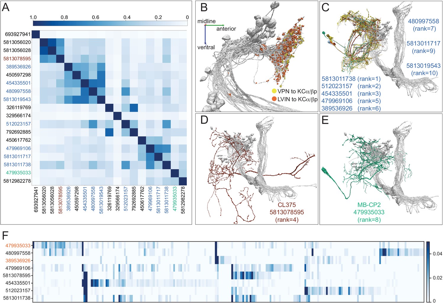
LVINs that conveys visual input onto α/βp KCs.
(A) A plot showing the cosine similarity of inputs to each of the 19 LVINs that most strongly connected (more than 20 synapses) to α/βp KCs. (B) An additional view of the distribution of VPN and LVIN inputs onto α/βp KCs. Note that LVIN input locations tend to be more posterior than those of VPNs. (C) Of the top 10 LVINs based on visual input delivered to α/βp KCs, eight are neurons with similar morphologies that fall into three cell types SLP360, SLP362 and SLP371, shown here. See Figure 11—figure supplement 3 for more morphological details of SLP371. (D) The LVIN conveying the fourth highest visual input to the dACA, CL375. (E) MB-CP2, the LVIN conveying the eighth highest visual input to the vACA; MB-CP2 (LHPV3c1) also provides 1% of input to KCs in the CA (see Figure 9). (F) A plot showing the similarity of VPN inputs for each of the top eight LVINs (using the ranking from panel A). Each vertical blue bar represents a different VPN and the intensity of the color reflects the percentage of the corresponding LVIN’s total VPN input that is contributed by that VPN. The order of the VPNs and LVINs was determined using spectral clustering.
Figure 11—figure supplement 3
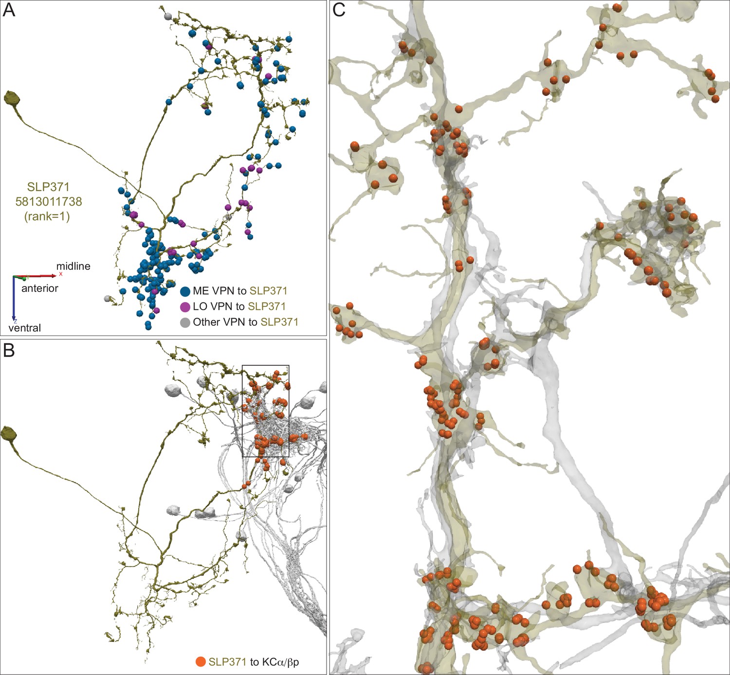
Detailed morphology of a dACA LVIN.
(A) One of the two SLP371 neurons (5813011738; green) is shown with the positions of its synaptic input from three color-coded classes of VPNs. (B) Synapses from this LVIN (green) onto the subset of α/βp KCs (gray) that it contacts are shown as orange dots. (C) Enlarged and rotated view of the box in (B). Note that connections from the LVIN to α/βp KCs lack the claw-like structure typical of the synapses between olfactory projection neurons and KCs in the CA.
Figure 11—figure supplement 4

Similarity of VPN inputs to individual LVINs that innervate the vACA or the dACA.
A heatmap showing the similarity of LVIN inputs from VPNs. It reveals the degree of diversity of the VPN inputs received by LVINs, as well as the existence of clusters of LVINs that receive similar inputs. Each square in the heat map represents a cosine similarity of the VPN inputs to a pair of LVINs. The ordering of the LVINs shown was determined by spectral clustering based on their inputs. Colors on the diagonals indicate whether the given LVIN is among the top 20 inputs to the vACA (green), to the dACA (pink), to both the vACA and dACA (orange), or neither (dark blue).
Figure 11—figure supplement 5
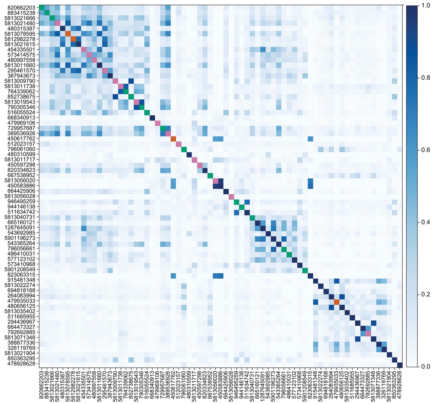
Similarity of non-visual inputs to individual LVINs.
A heatmap in the same format as Figure 11—figure supplement 4 but showing the similarity of LVIN inputs from non-visual (i.e. non-VPN, non-LVIN) neurons. LVINs are shown in the same order as in Figure 11—figure supplement 4. The fact that substantial structure is preserved between these plots indicates that clusters of LVINs with similar visual inputs also tend to receive similar inputs from neurons that do not (directly) relay visual information. Colors on the diagonals indicate whether the given LVIN is among the top 20 inputs to the vACA (green), to the dACA (pink), to both the vACA and dACA (orange), or neither (dark blue).
Figure 12 with 2 supplements
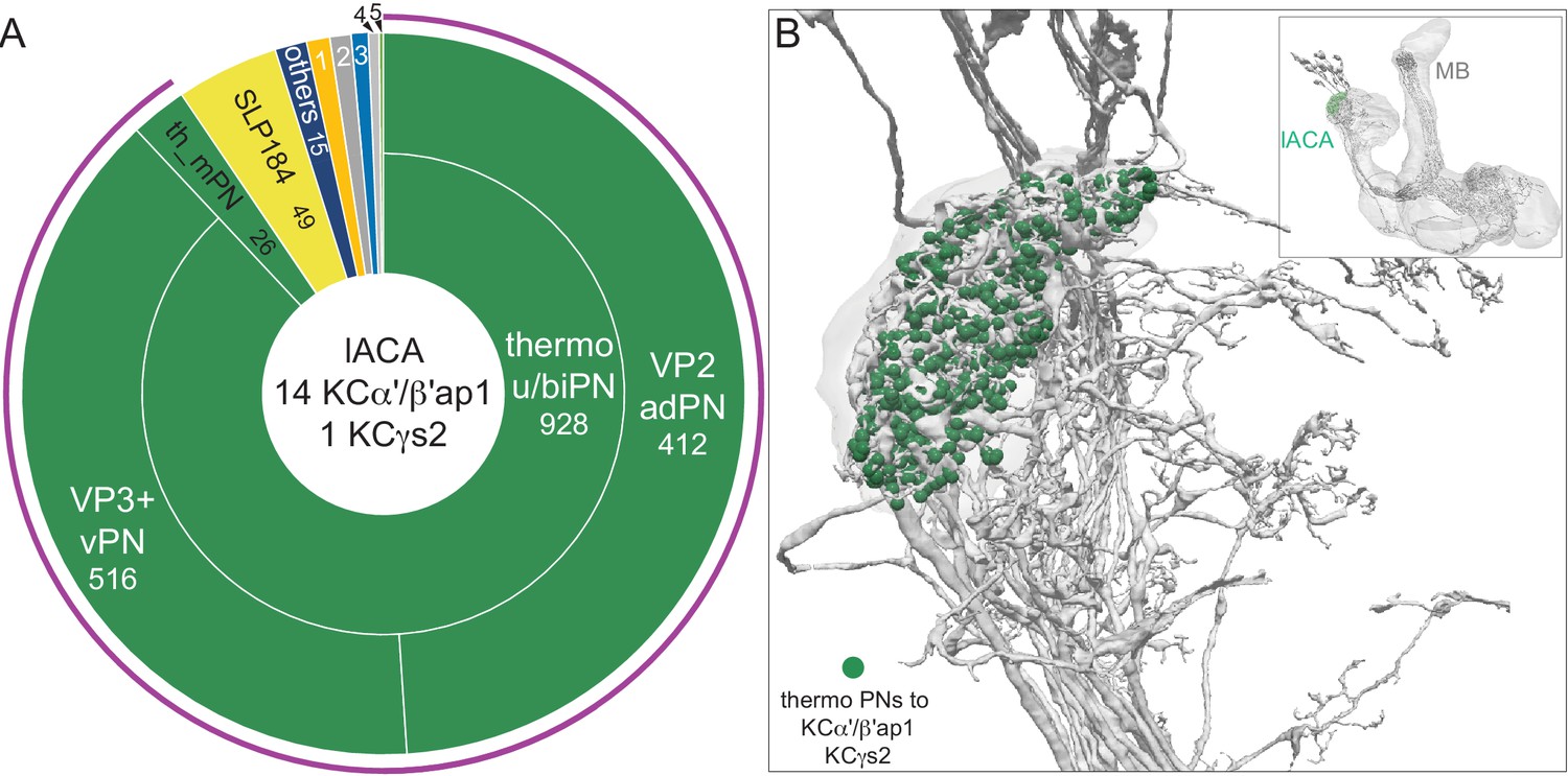
Lateral accessory calyx (lACA).
The lACA is defined by the limits of the presynaptic boutons of VP2 adPN (1975878958) and VP3+ vPN (663432544); there also appear to be glia separating the lACA from main CA. Fourteen α′/β′ap1 KCs and the γs2 KC innervate the lACA. (A). A pie chart showing inputs to the 15 lACA-innervating KCs. The majority of input to these KCs is from the two thermosensory uPNs, VP2 adPN and VP3+ vPN, that contribute 928 synapses, of which the single γs2 KC receives 268. Other prominent inputs are one local interneuron (SLP184) and two thermo/hygrosensory mPNs. Eight interneurons (other) contribute 15 synapses. Sources of input indicated by the other numbered sectors are as follows: 1, circadian clock-associated neurons (1.0%); 2, APL (0.9%); 3, MB-C1 (0.7%); 4, KC-to-KC connections and 5, other PNs (0.2%). The total temperature information presented to KCs by PNs is indicated by the purple arc around the outer layer. Note that KCs in lACA have dramatically less KC-to-KC and APL input than those in the dACA and the vACA. (B) Synaptic connections from thermo uPNs (green) to KCs (gray). The inset shows the orientation of the MB.
Figure 12—figure supplement 1
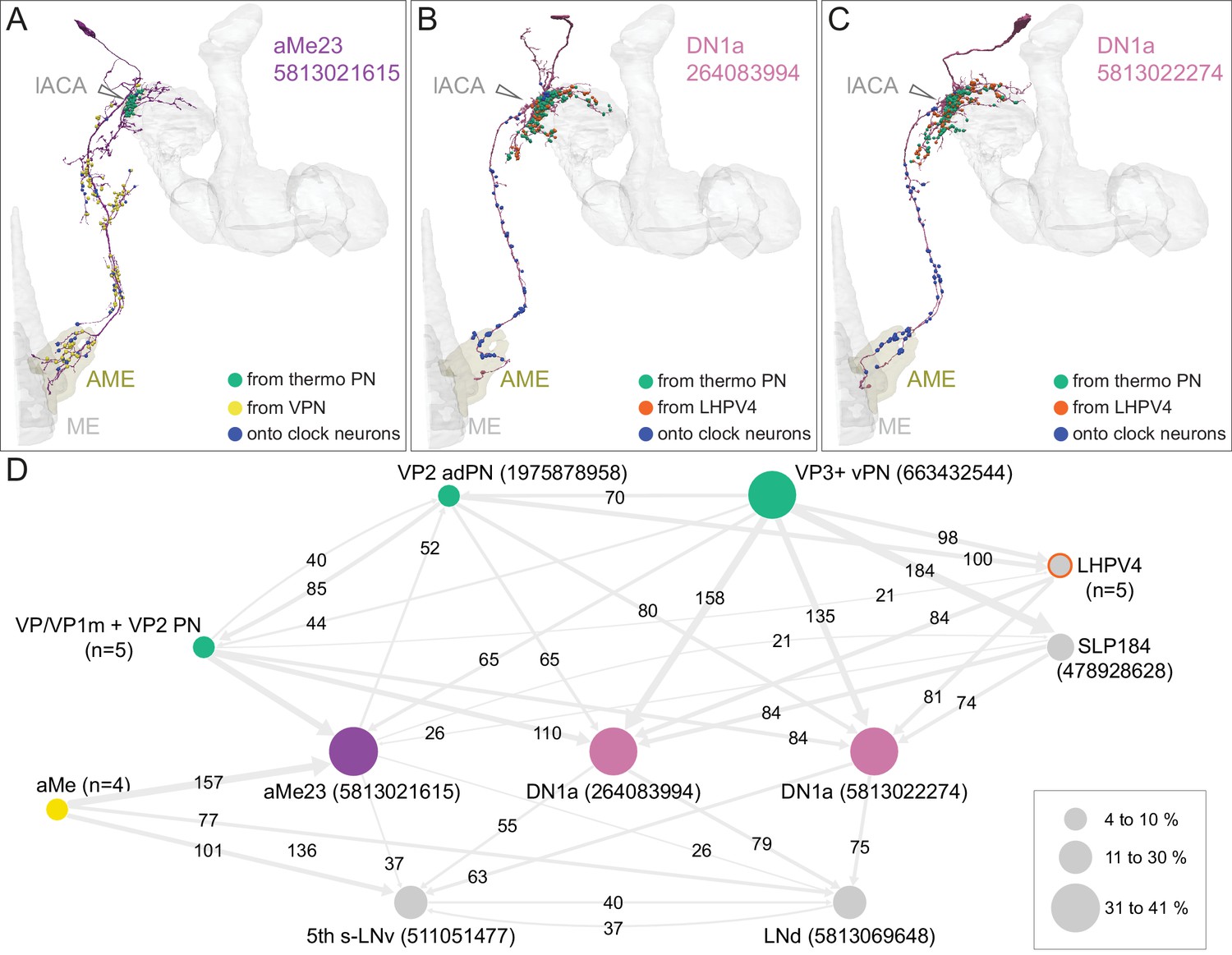
DN1a and DNa1-like (aMe23) neurons relay temperature cues from the lACA to the circadian clock.
(A) Morphology of a DNa1-like neuron (aMe23) with the positions where it receives thermosensory input in the lACA (green) and visual inputs (yellow) in the accessory medulla (AME) and the PLP. The positions of its synapses onto two clock neurons, the 5th s-LNv and one LNd, are shown in blue. (B–C) Morphologies of two DN1a neurons with inputs from thermosensory PNs and the LHPV4 interneurons, as well as outputs to the same two clock neurons 5th s-LNv and LNd, shown color-coded. (D) Simplified circuit diagram. The aMe23 and DN1a neurons show different patterns of input from visual projection neurons (aMe; yellow), thermosensory and hygrosensory projection neurons (VP/VP1m + VP2 PN, VP3+ vPN, VP2 adPN; green), and interneurons (LHPV4; gray with red outline) (Marin et al., 2020). Temperature entrainment of the circadian clock requires input from the aristae (Yadlapalli et al., 2018; Alpert et al., 2020), which house the VP3 and VP2 sensory neurons (Gallio et al., 2011); the connections we observed provide a potential anatomical substrate for arista-dependent temperature entrainment of the clock. DN1a (Helfrich-Förster, 2004; Shafer et al., 2006) and aMe23 neurons provide input to the circadian clock neurons 5th s-LNv and LNd. Connections of fewer than 20 synapses have been omitted. The sizes of the three green circles representing PN types indicate the percentage of those neurons’ total output (based on synapse number) going directly to other neurons in the diagram; the sizes of the circles representing all other neurons indicate what percent of that neuron’s total input comes directly from other neurons in the diagram.
Figure 12—figure supplement 2
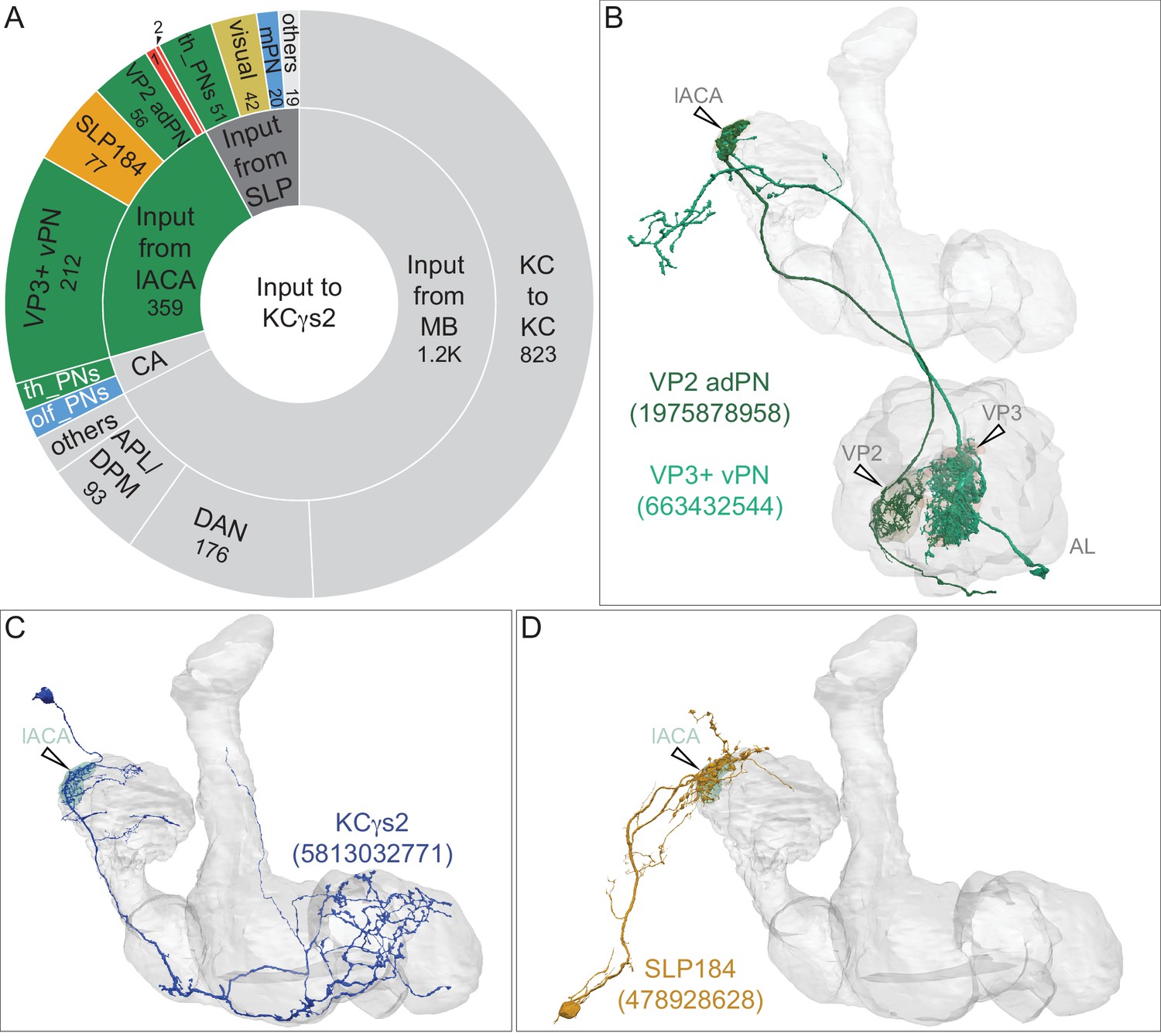
KCγs2 and its inputs.
(A) Distribution of inputs to KCγs2. KCγs2 receives the vast majority of its sensory input in the lACA from thermo/hygrosensory PNs, but also receives a small amount of visual and olfactory information. Note that the pie chart reflects all of KCγs2’s inputs, not just those that occur in the lACA. KCγs2 receives nearly half its input from putative KC-to-KC synapses in the γ lobe. The γs2 KC receives the majority of its sensory input in the lACA from two thermal PNs (VP3+ vPN and VP2 adPN); other lACA inputs include the interneuron SLP184 (4.5%) and neurons represented by the numbered sectors: 1, aMe23 (10, 0.7%) and 2, VP1m+VP2_lvPN2 (8, 0.5%). The γs2 KC also receives 132 synapses (7.7% of its input) from its arbor that lies in the SLP, outside main CA and lACA, indicated in the gray wedge, as well as a small amount of input from other thermal and olfactory PNs in the CA. (B) Morphologies of thermosensory PNs VP2 adPN and VP3+ vPN, which are the major inputs to the lACA, are shown. (C) Morphology of KCγs2. (D) Morphology of the interneuron SLP184.
Figure 13 with 2 supplements
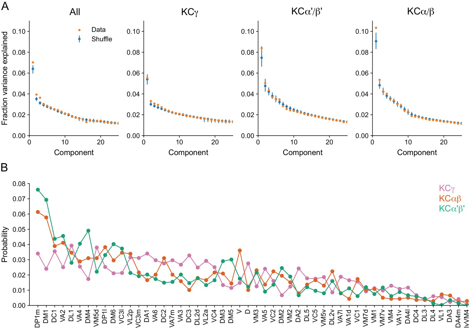
Comparison of KC input connectivity to random models.
(A) Fraction of variance explained by components identified via principal components analysis of the olfactory uPN-to-KC input connectivity matrix—a binary matrix containing ones and zeros for present or absent connections between KCs and their inputs, at a threshold of five synapses. Results are shown for the reconstructed data (orange) and for a collection of shuffled models (blue) in which each KC retains the same total number of connections but samples among all uPNs randomly, with a probability proportional to the total number of connections each uPN makes. Such models therefore retain the degree distribution across KCs, (that is, the probability distribution of the number of claws formed by individual KCs) and the average connection probability for each uPN, but no other structure. Bars indicate 95% confidence intervals for shuffled models. Deviations in the first few components indicate structure inconsistent with a random model. Left: All KCs; Right: Analysis restricted to the indicated KC subtypes (visual α/βp and γd KCs, as well as γs KCs, were excluded). (B) Probability of uPN-to-KC connections from each olfactory glomerulus, sorted by most to least well-connected. Probabilities are plotted separately for the KC subtypes shown in (A).
Figure 13—figure supplement 1
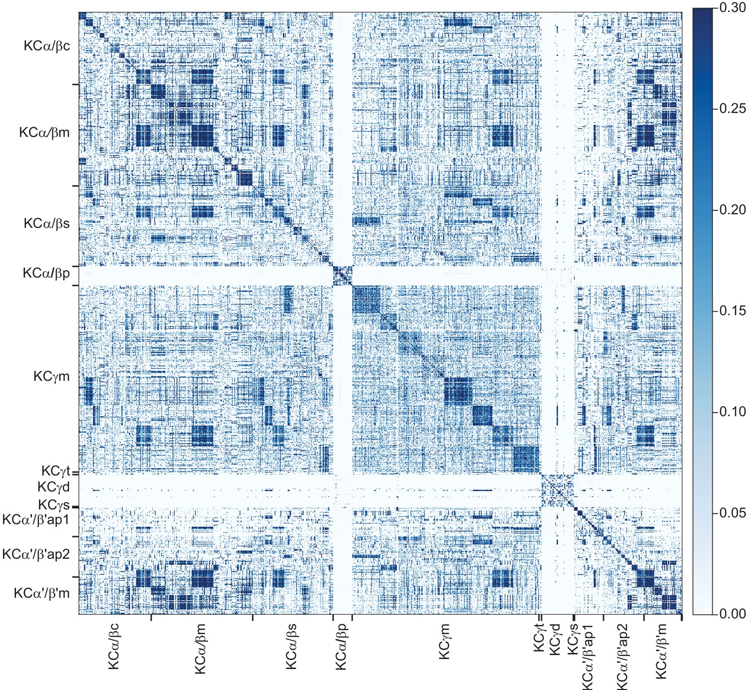
Clustering KCs based on the similarity of their inputs from PNs.
Cosine similarity of PN inputs to KCs. This metric measures the degree of overlap in the PN inputs, weighted by synapse count, to each pair of KCs. Each PN is treated individually, rather than being grouped by cell type. KCs are grouped by subtype, and then the ordering within each subtype is determined by spectral clustering. The optimal number of clusters within each type is determined using the silhouette score and capped at 10. The potential computational significance of groups of KCs responsible for distinct PN inputs is modeled in Figure 38.
Figure 13—figure supplement 2
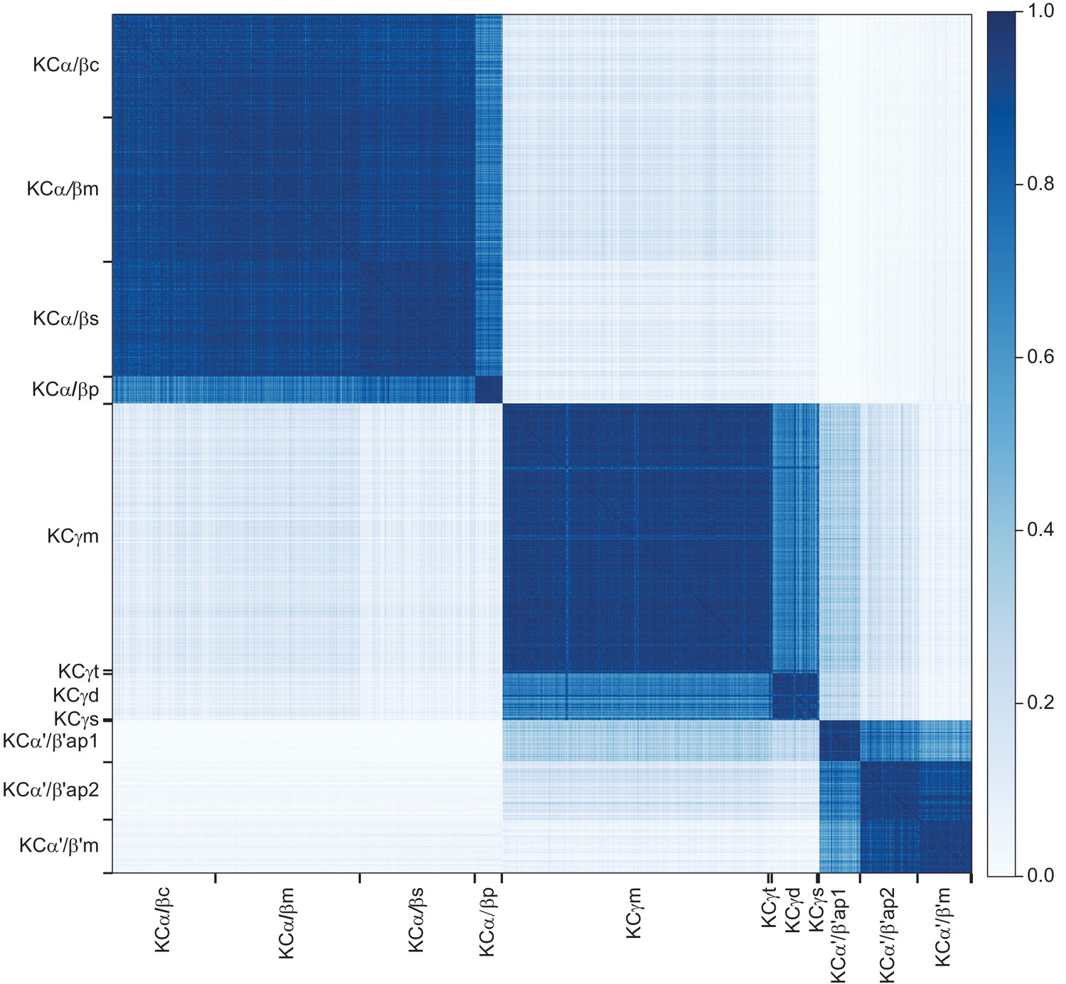
Similarity of KC outputs to MBONs.
Cosine similarity of KC outputs to MBONs. KCs are grouped by subtype, and then indexed in the same order as in Figure 13—figure supplement 1.
Figure 14
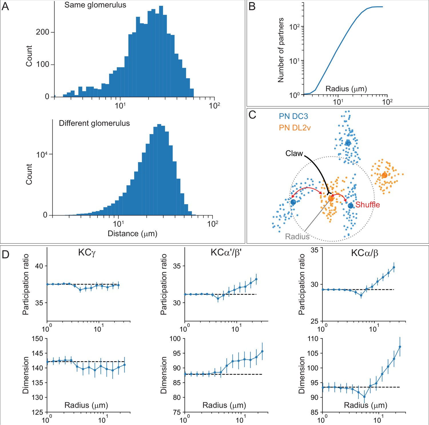
Effect of spatial organization on the KC representation.
(A) Histogram of pairwise distances between boutons formed by PNs from the same glomerulus (top) or different glomeruli (bottom). (B) Average number of nearby boutons within a given radius of each PN bouton. (C) Illustration of shuffling procedure used to randomize PN-to-KC connectivity within a given radius. Small dots: S ynapses formed by each PN onto KCs. Large dots: Centroid location of identified boutons. Claws are randomly reassigned (red arrows) to boutons whose centroids lie within the given radius, indicated by the dotted gray line. (D) Participation ratio (top) and dimension (bottom) of models constructed by shuffling connectivity within a specific radius. The dependence of these two quantities on the shuffle radius shows a modest effect of the spatial organization of the CA on the KC representation in the model.
Figure 15 with 3 supplements
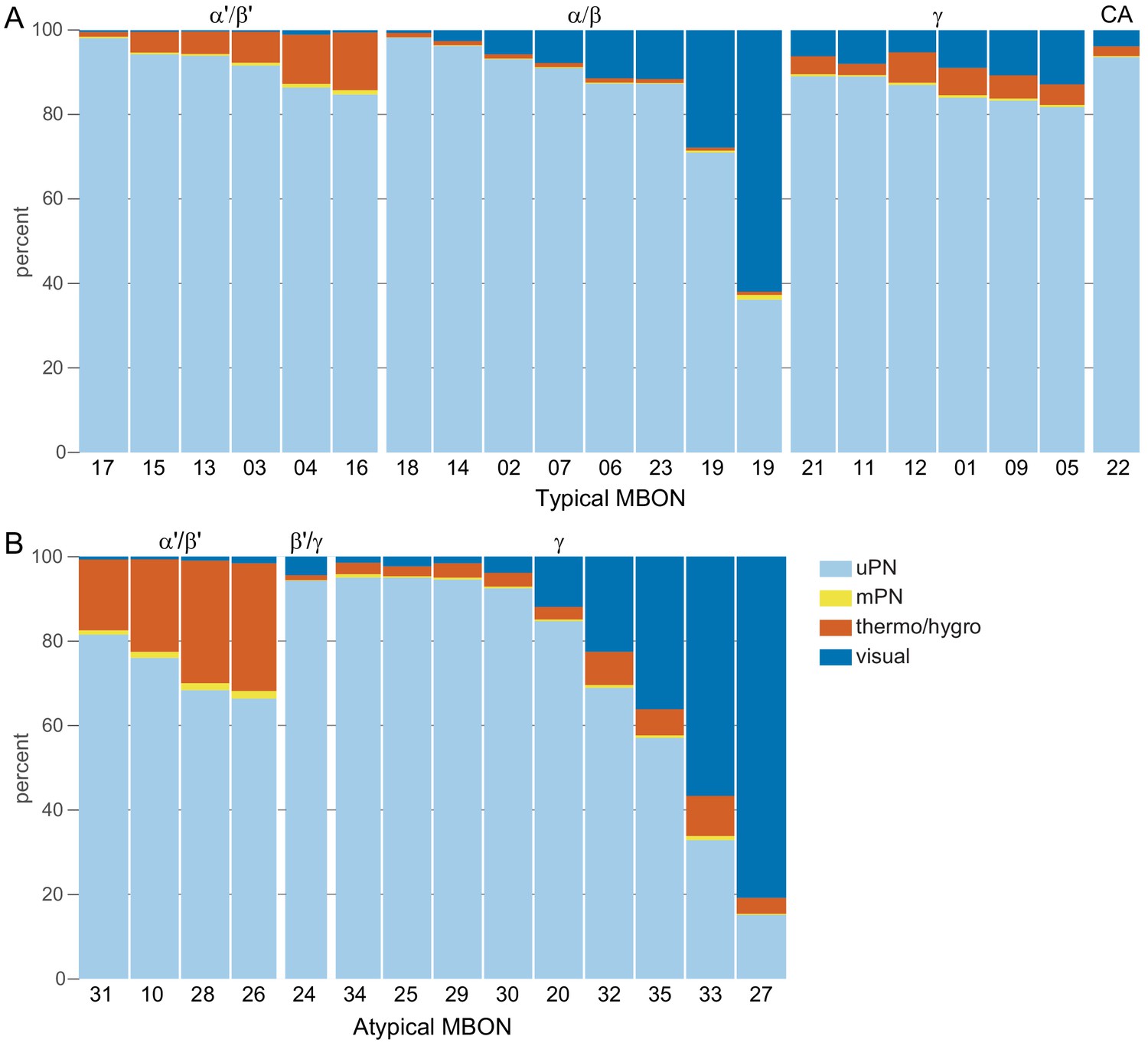
Structure in PN-KC-MBON connectivity.
(A) Effective PN-to-MBON connectivity. MBONs within the α′/β′ lobe receive input primarily from uniglomerular olfactory PNs (uPNs), but they also show a gradation of input from thermo-hygrosensory PNs. MBONs from the α/β lobes show a similar, although stronger, variation in the amount of input they receive from visual PNs. MBONs from the γ lobe are more uniformly innervated. For cases where the MBON cell type contains more than one cell, results from the individual cells have been averaged in this figure, with the exception of the two MBON19 (α2p3p)s; both MBON19s are specialized for visual input, but to different extents. (B) Effective PN to atypical MBON connectivity. The gradation in non-olfactory input is stronger than for typical MBONs. In particular, the majority of the input to MBON33 (γ2γ3) and MBON27 (γ5d) is visual. In this figure and its supplements, the MBONs have been grouped by the MB lobe they primarily innervate and then ordered, within these groups, according to their selectivity. MBON24 (β2γ5) receives input from both the β and γ lobes. Percentages indicate the amount of input to each MBON from a particular PN type divided by the total sensory input to that MBON.
Figure 15—figure supplement 1

PN connections to KC types and effective PN-to-MBON connectivity.
Detailed views of the PN inputs to KCs and MBONs. The uPN types are listed individually. Inputs from multiglomerular PNs (mPN), thermo/hygrosensory (thermo) and visual pathways have been pooled over all input neurons of each type. Percentages indicate the amount of effective input due to a particular PN type divided by the total sensory input to each target cell or population; the thermo-hygrosensory and visual results have been divided by the factors indicated in each column, to keep the color scale within reasonable bounds. (A) Inputs from uPNs, mPNs, thermo/hygrosensory and visual pathways to KCs of different subtypes. (B) Inputs from uPNs, mPNs, thermo/hygrosensory and visual pathways to each typical MBON. (C) The same plot as in (B), but for the atypical MBONs. Note that this plot reflects only input that atypical MBONs receive from KCs and ignores other input that they receive from their dendrites that extend outside the MB lobes. Approximately 80 and 55% of the inputs to MBON27 (γ5d) and MBON33 (γ2γ3), respectively, convey visual information (see Figure 15B). Note that input from VC5 and VL2p is highly represented by the same MBONs that receive strong input from thermo-hygrosensory PNs, supporting the idea that these glomeruli may also convey thermo-hygrosensory information (Hamada et al., 2008; Frank et al., 2015; Marin et al., 2020).
Figure 15—figure supplement 2
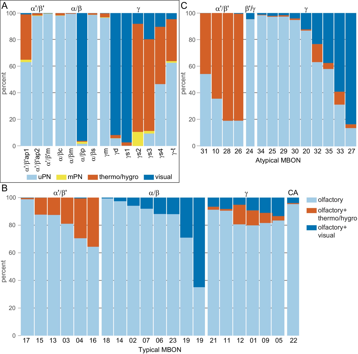
PN-to-KC and KC-to-MBON connectivity by sensory modality.
(A) Olfactory input from uniglomerular PNs is carried by most of the KC types (α′/β′m, α′/β′ap2, α/βc, α/βm, α/βs, γm), but thermo/hygrosensory and visual inputs are conveyed by specific KC subtypes. In particular α/βp, γd, and γs1 KCs carry substantial fractions of visual input, and α′/β′ap1, γs2-4, and γt KCs convey thermo-hygrosensory information. (B) Within the α′/β′, α/β, and γ lobes, the amount of non-olfactory input to different typical MBONs varies across MBON types due to differential KC innervation. Typical MBONs innervating the α′/β′ lobe receive variable amounts of thermo-hygrosensory input due to different levels of α′/β′ap1 innervation. Visual input varies across the α/β MBONs due to different amounts of α/βp KC input. The γ lobe, in contrast, has a more uniform distribution of different sensory modalities across its typical MBONs. (C) Same as (B), but for atypical MBONs. Percentages indicate the number of synapses of a given type divided by the total number of sensory input synapses to each KC type (panel A) or KC synapses to each MBON (panels B and C). Panels B and C reflect KC input to MBONs with the KCs divided into classes according to panel A. In contrast, Figure 15 show the full input-to-output effective connectivity.
Figure 15—figure supplement 3
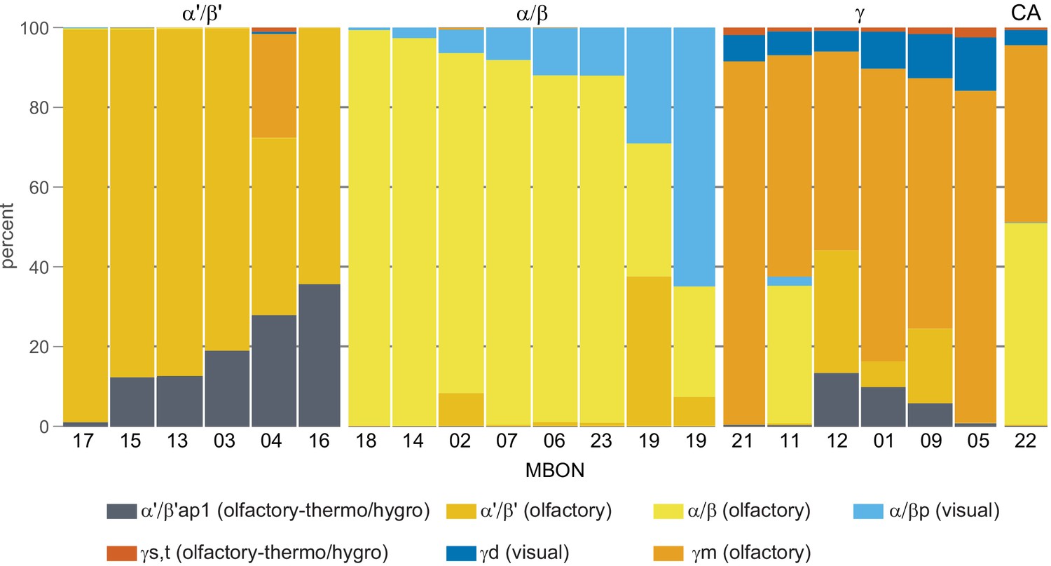
MBON connectivity by KC type.
Percentage of input to typical MBONs by KC type. Similar to Figure 15—figure supplement 2C, except that the KCs have been divided by lobes as well as by sensory modality. MBONs exhibit different biases toward KC types, which underlies the differences (as shown in Figure 15—figure supplement 2) in the proportion of effective input they receive from each sensory modality. We also observe a few instances of MBONs receiving substantial input from KCs in unexpected (relative to prior findings) lobes, including the large percentage of γ KC input to MBON04 (β′2mp_bilateral), and the large percentages of α′/β′ input to one of the two MBON19s (α2p3p). It is unknown if these unexpected connections are stereotyped.
Figure 16 with 4 supplements

MBON input and output similarity structure.
A comparison of MBON inputs and outputs through the lens of similarity structure. Left: cosine similarity of MBONs based on their effective PN inputs via KCs (computed as in Figure 15). Each cell of the heat map indicates the input similarity of the indicated pair of MBONs. A value of 0.5 indicates that the PN subpopulations conveying input to the two MBONs via KCs are half overlapping and half disjoint. Right: cosine similarity of MBONs based on their outputs to all neurons (unnamed neuronal fragments have been excluded). The resemblance between the left and right plots suggests that MBON outputs preserve some of the parallel structure in the PN-KC-MBON pathway. In each plot, the square in the diagonal is color-coded to indicate the MB lobe in which that MBON’s dendrites lie. The MBON names are color-coded to indicate their neurotransmitter, as indicated.
Figure 16—figure supplement 1
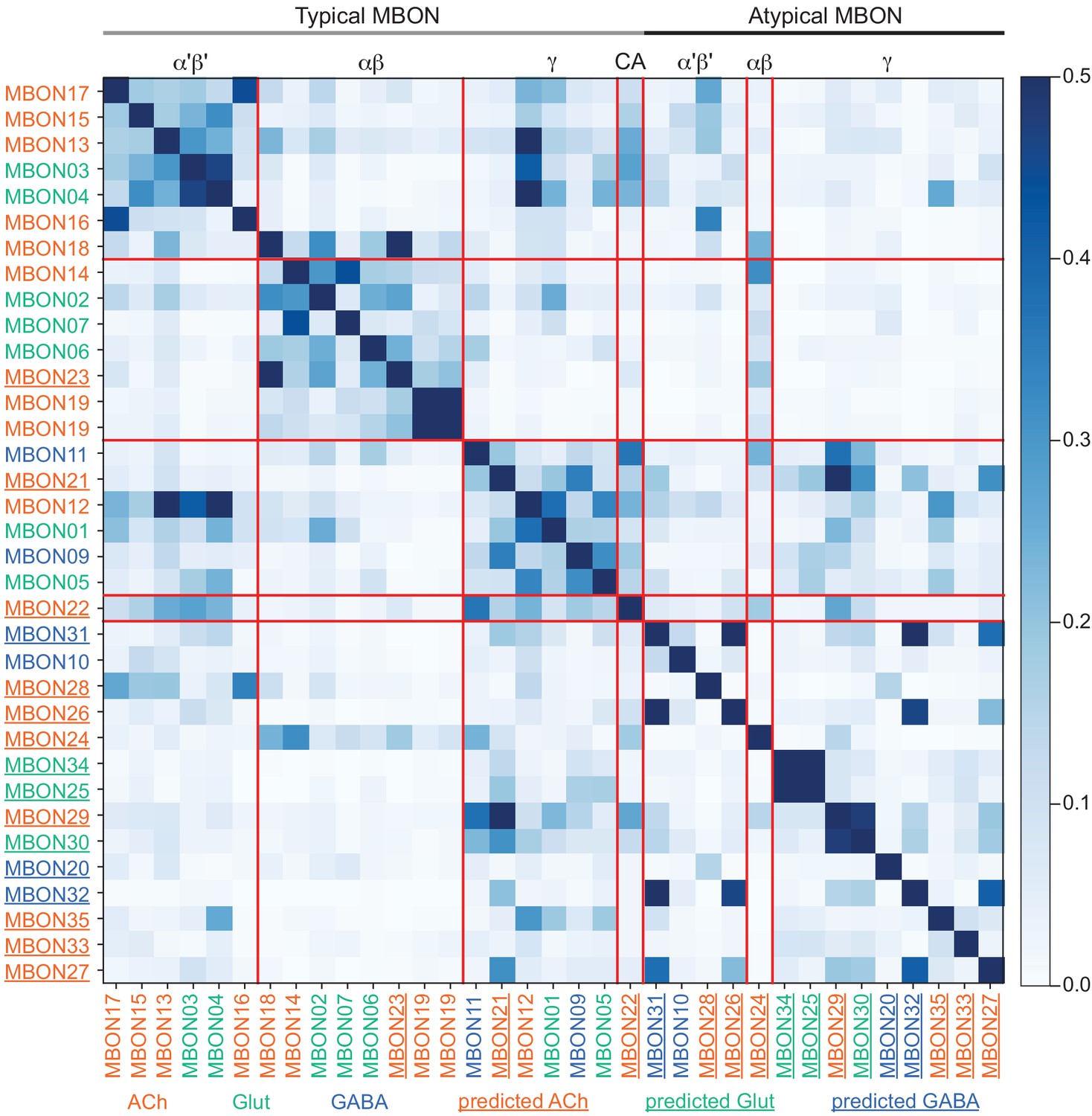
MBON output similarity by lobe.
Cosine similarity of MBONs based on the similarity of their outputs to all neurons (unnamed neuronal fragments have been excluded). Each cell of the heat map indicates the output similarity of the indicated pair of MBONs. This is the same data as plotted in Figure 16, except that the MBONs are organized by lobe, shown in the same order as in Figure 15. The preservation of lobe-wise sensory input structure in the MBONs suggests that MBONs may mediate multiple parallel pathways that transform sensory information into behavioral output. The MBON names are color-coded to indicate their neurotransmitter, as indicated.
Figure 16—figure supplement 2
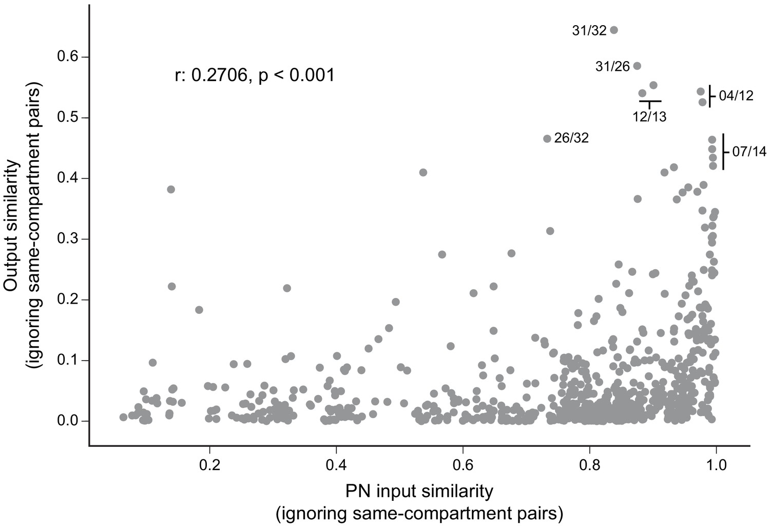
Correlation of MBON output and PN input similarity.
Scatter plot of MBON output similarity vs. similarity of their inputs from PNs, quantifying the relationship between the structure of MBON outputs and their sensory inputs. Each point represents a pair of MBONs from different compartments. Output similarity is computed using the cosine similarity of outputs, as in Figure 16. PN input similarity is computed using cosine similarity of effective PN inputs, as in Figure 16. The highest 10 points on the y-axis correspond to the following pairs (fewer than 10 listed due to multiple MBONs of the same type): MBON31 (α′1a) and MBON32 (γ2); MBON26 (β′2d) and MBON31 (α′1a); MBON12 (γ2α'1) and MBON13 (α′2); MBON04 (β′2mp_bilateral) and MBON12 (γ2α′1); MBON26 (β′2d) and MBON32 (γ2); MBON07 (α1) and MBON14 (α3).
Figure 16—figure supplement 3
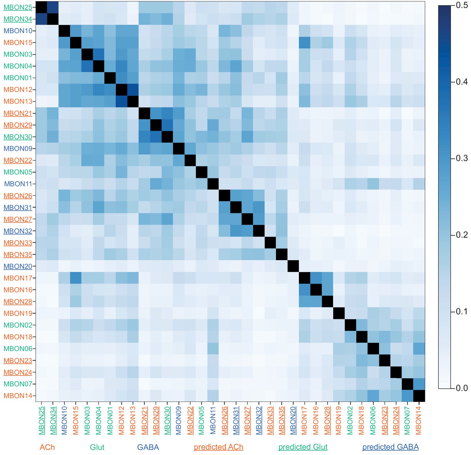
MBONs clustered by output similarity.
Cosine similarity between each MBON type and their target population. The ordering of MBONs was determined using average clustering. Unlike Figure 16 or Figure 16—figure supplement 1, the ordering of the MBONs in this figure does not take into account input structure or anatomical structure, allowing for unbiased grouping of MBONs based on their outputs. This reveals some clusters of MBONs with convergent outputs that span multiple lobes. Only named neurons were considered in the target population. MBON names are color-coded by neurotransmitter with predicted transmitters also underlined.
Figure 16—figure supplement 4
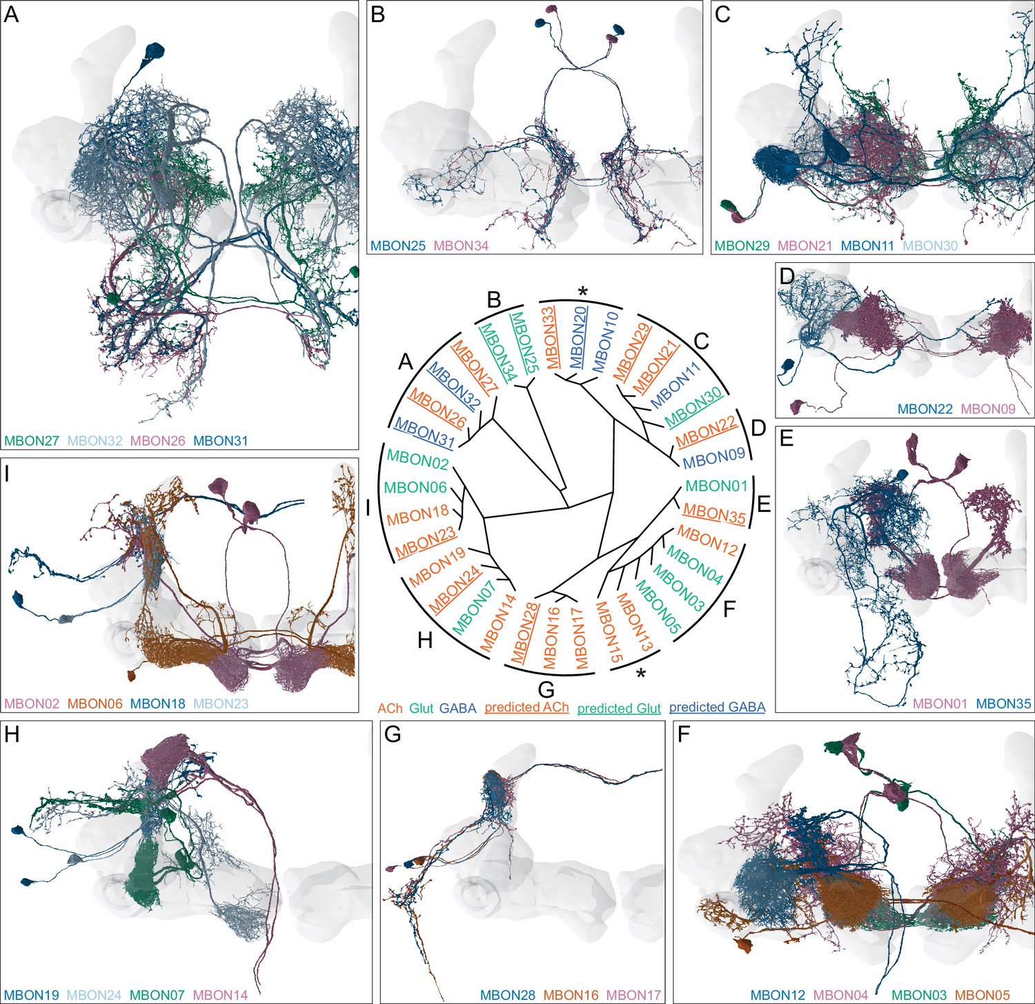
MBON morphologies grouped by output similarity.
Radial dendrogram shows that MBONs with similar downstream connectivity innervate different compartments. A dendrogram based on the MBON cosine similarity matrix (Figure 16—figure supplement 3) was extracted and the morphologies of the MBON in each group were plotted. Colored MBON names in each panel match the colors of the MBONs in the morphology images. MBONs can have similar downstream connectivity regardless of whether they innervate the same (MBONs 16, 17, and 28) or different (MBONs 23, 18, 06, and 02) compartments. The asterisk indicates MBONs (MBON10, 13, 15, 20, and 33) that could not be grouped with another partner; they are singletons where their downstream connectivity is different from all other MBONs.
Figure 17 with 1 supplement
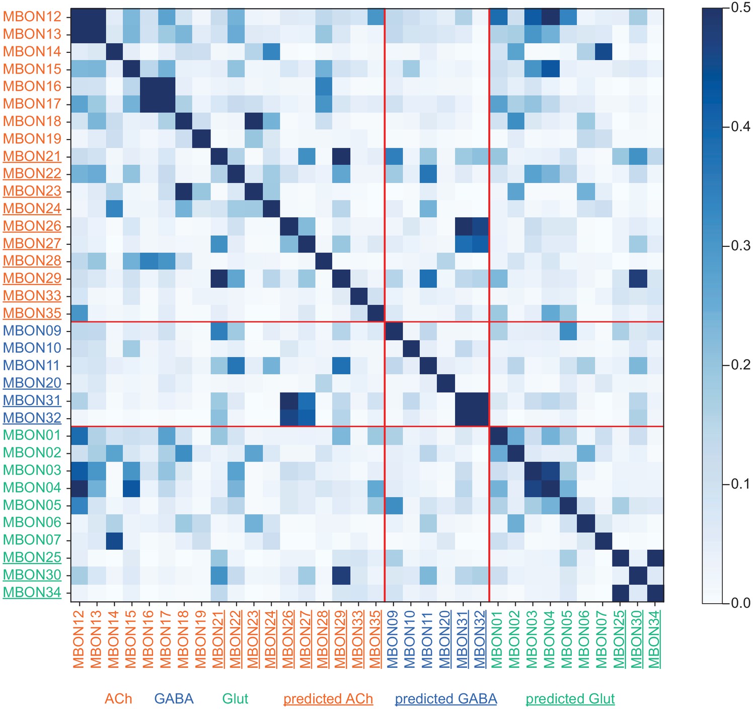
MBON output similarity by neurotransmitter.
Cosine similarity of MBON outputs to all named neurons. MBONs have been grouped by neurotransmitter and then presented in numerical order. There exist many instances of convergent outputs between cholinergic and glutamatergic neurons, suggesting a widespread ‘push-pull’ motif in MBON output convergence patterns. This phenomenon is emphasized in Figure 17—figure supplement 1 and notable examples are explored in further detail in Figure 20—figure supplement 1 and Figure 21—figure supplements 1,2. The MBON names are color-coded by neurotransmitter with predicted transmitters underlined.
Figure 17—figure supplement 1
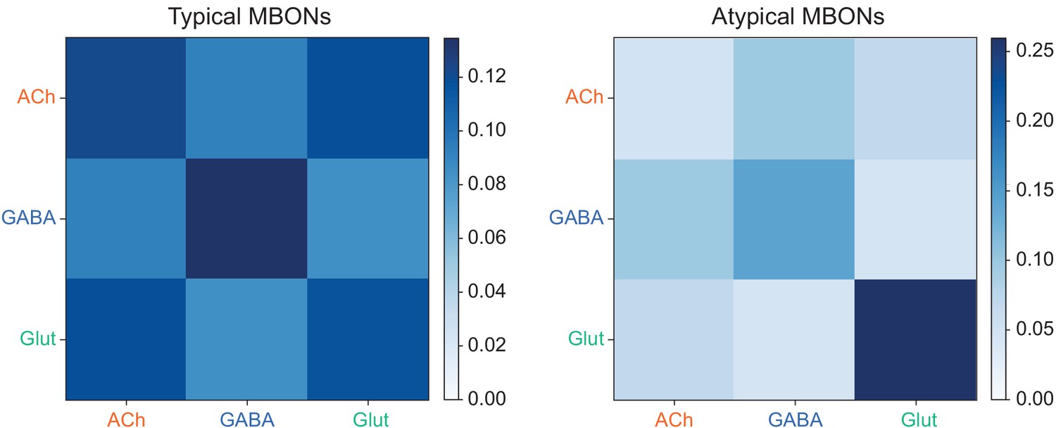
MBON output similarity pooled by neurotransmitter.
Average cosine similarity of pairs of MBONs computed by collapsing the blocks in Figure 17 after separating typical and atypical MBONs. Note that the heat-map scale is different in the two plots.
Figure 18 with 3 supplements
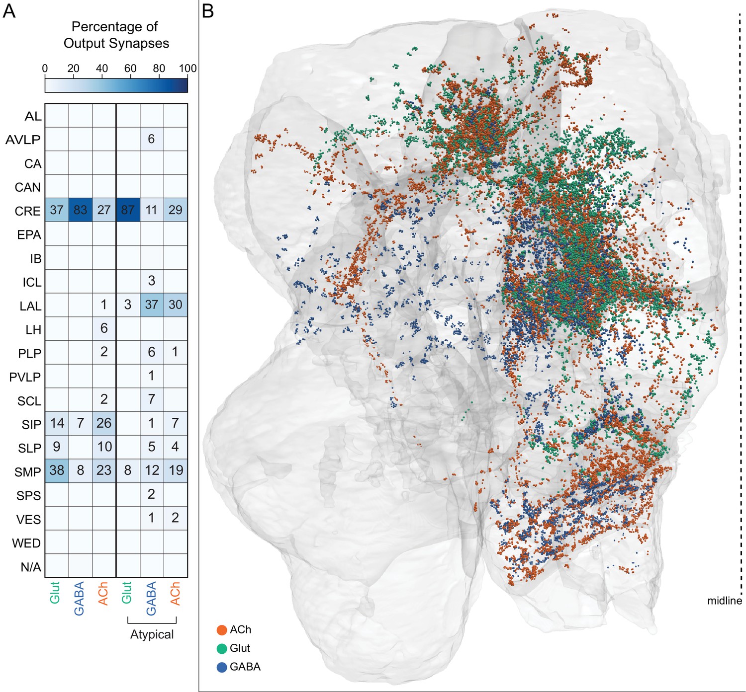
MBON output distribution by neurotransmitter.
(A) Table indicating the percentage of output synapses of each MBON neurotransmitter type, including predicted neurotransmitters, that reside in the given brain area; typical and atypical MBONs were analyzed separately. (B) Visualization of the spatial position of MBON output synapses throughout the hemibrain volume, color-coded by neurotransmitter type. Figure 18—figure supplement 1 shows the same data presented on separated brain areas. Figure 18—figure supplement 2 shows data for individual MBONs pooled by brain area. Figure 18—figure supplement 3 shows the same data as Figure 18, but with predicted neurotransmitters shown in gray.
Figure 18—figure supplement 1

MBON output distribution by neurotransmitter presented on separated brain areas.
Visualization of the spatial position of MBON output synapses within individual brain areas.
Figure 18—figure supplement 2
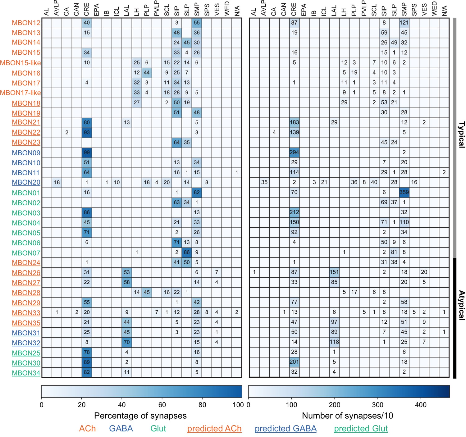
Distribution of individual MBON outputs by brain area.
(Left) The value of each cell indicates the percentage of the given MBON’s output synapses that reside in the given brain area. Blank cells indicate values of less than 1%. (Right) The value of each cell indicates the number of the given MBON’s output synapses that reside in the given brain region divided by 10 and rounded to an integer. Blank cells indicate brain regions that receive fewer than 10 synapses from the corresponding MBON.
Figure 18—figure supplement 3
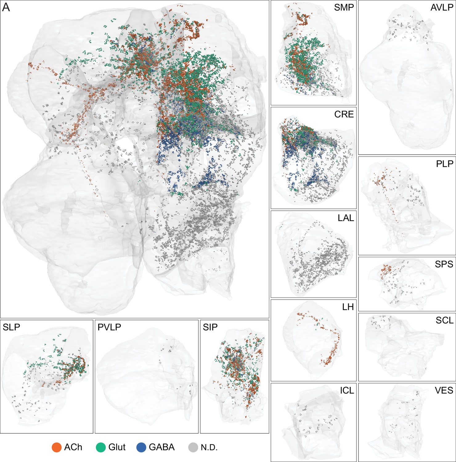
Same plot as in Figure 18 but with only synapses from neurons whose neurotransmitters had been confirmed by antibody staining ( Aso et al., 2014a) shown color-coded.
Other synapses shown in gray.
Figure 19 with 1 supplement
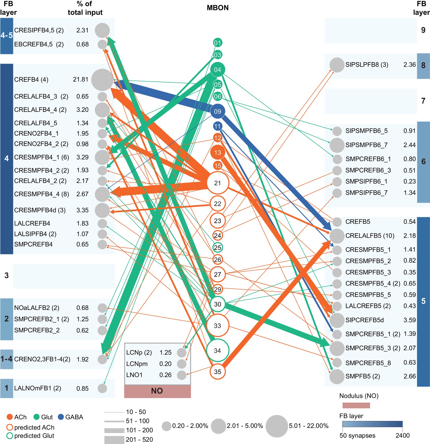
Direct connections from MBONs to the central complex (CX).
In this diagram, the central column shows those MBONs that make direct connections of 10 or more synapses onto the dendrites of CX neurons. Such direct connections predominantly occur on fan-shaped body (FB) neurons. Three cell types of nodulus (NO) cell types are also direct targets (see Figure 19—figure supplement 1A); some FB cell types in layers 1, 2, 3, and 4 that are downstream of MBONs also have arbors in the NO. No direct targets were identified in other CX neuropils such as the ellipsoid body (EB) or protocerebral bridge (PB). The number in the circle indicates the MBON cell type; that is, 01 stands for MBON01. The size of the circle indicates what percent of that MBON’s total output (based on synapse number) goes directly to FB neurons. The color of solid circles represents confirmed neurotransmitter types while the color of the outline of hollow circles represents predicted neurotransmitter types. Numbers have been pooled for cases where there are multiple MBONs of the same cell type. The outer columns show FB cell types, arranged by FB layer(s). The name of the cell type and, in parentheses, the number of cells of that type are indicated for those with multiple cells. The percentage of that cell type’s input that comes from MBONs is given and is reflected by the size of the circle representing the cell type. All FB neuron types receive less than 5% of their total input from MBONs except for one layer 4 FB neuron type, CREFB4 (FB4R), which receives nearly 20% of its inputs from two MBONs, MBON09, and MBON21 (see Figure 19—figure supplement 1B,C). Direct MBON connections to the FB are concentrated in FB layers 4 and 5. Links to each of these FB and NO cell types in neuPrint, listed from FB layer 1 to FB layer 9 and then for the nodulus, are as follows: LALNOmFB1 (FB1C), CRENO2,3FB1-4 (FB1H), NOaLALFB2 (FB2A), SMPCREFB2_1 (FB2C), SMPCREFB2_2 (FB2L), CRESMPFB4_1 (FB4A), CRENO2FB4_1 (FB4C), CRESMPFB4_2 (FB4D), CRELALFB4_2 (FB4F_b), CRELALFB4_3 (FB4G), CRELALFB4_4 (FB4H), LALCREFB4 (FB4I), CRELALFB4_5 (FB4J), LALSIPFB4 (FB4L), CRENO2FB4_2 (FB4M), SMPCREFB4 (FB4N), CRESMPFB4d (FB4O), CRESMPFB4_4 (FB4P_a and FB4P_b), CREFB4 (FB4R), CRESIPFB4,5 (FB4X), EBCREFB4,5 (FB4Y), LALCREFB5 (FB5A), SIPCREFB5d (FB5AB), SMPCREFB5_1 (FB5C), CRESMPFB5_1 (FB5D), CRESMPFB5_2 (FB5E), CRESMPFB5_3 (FB5H), SMPCREFB5_3 (FB5I), SMPFB5 (FB5J), CREFB5 (FB5K), CRESMPFB5_4 (FB5L), CRESMPFB5_5 (FB5M), CRELALFB5 (FB5V), SMPCREFB5_8 (FB5X), SMPSIPFB6_1 (FB6A), SMPCREFB6_1 (FB6P), SIPSMPFB6_5 (FB6Q), SMPSIPFB6_7 (FB6R), SIPSMPFB6_7 (FB6T), SMPCREFB6_3 (FB6V), SIPSLPFB8 (FB8F_a), LCNp (LCNOp ), LCNpm (LCNOpm), and LNO1 (LNO2).
Figure 19—figure supplement 1
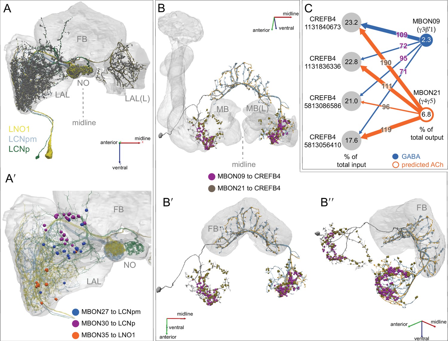
The morphology and connectivity of nodulus and CREFB4 neurons.
(A) Morphologies of the LCNp (LCNOp), LCNpm (LCNOpm), and LNO1 (LNO2) nodulus neurons that are downstream of MBONs. The FB, NO, and LAL are shown in gray. Presynaptic sites are shown as yellow dots and postsynaptic sites as gray dots. (A′) Higher magnification view, showing the locations of MBON inputs onto these neurons. (B) CREFB4 (FB4R) neurons are shown with each of the four neurons of this type displayed in a different color. The locations of the synapses CREFB4 (FB4R) cells receive from MBON09 (γ3β′1) and MBON21 are shown, color-coded. (B′-B′′) Alternative views of image shown in (B). (C) Diagram of synaptic connectivity. The numbers in the circles that represent the cells indicate, for CREFB4 (FB4R) cells, the percentage of their input that comes from these two MBONs and, for the MBONs, the percent of their output that goes to CREFB4 (FB4R). The numbers in the arrows are the number of input synapses. The neurotransmitters of the MBONs are indicated.
Figure 20 with 5 supplements
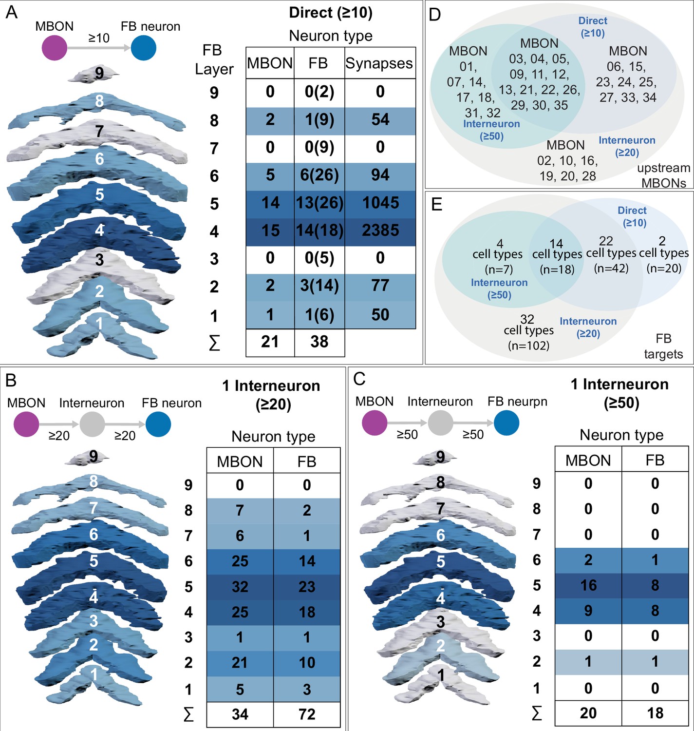
Summary of connections from MBONs to the FB.
Heat maps are shown that compare the strength of connection between MBONs and FB neurons in each FB layer. (A) Direct connections. The number of MBON cell types within each layer that make synapses onto the dendrites of FB neurons, the number of FB neuron types (also within the indicated layers) they connect to, and the total number of MBON to FB neuron synapses are shown for each FB layer. The total number of cell types listed in neuPrint for each FB layer is shown in parentheses. The last row of the table shows the number of different MBON cell types that make direct connections to the FB; some MBONs connect to more than one layer. (B,C) Connections using a single interneuron. The number of MBON cell types connecting to each layer and the number of FB neuron types they connect to are shown. Connections between the MBON and the interneuron as well as between the interneuron and the FB neuron are required to have 20 or more synapses (B) or 50 or more synapses (C). The last row of the table shows the number of different MBON cell types that make indirect connections to the FB at this threshold; some MBONs connect to more than one layer. (D) Venn diagram comparing MBON types that are connected to FB neurons directly (as in A); through one interneuron with threshold of 20 synapses (as in B); and through one interneuron with threshold of 50 synapses (as in C). (E) Venn diagram comparing FB cell types that are targeted by MBONs directly (as in A), through one interneuron with threshold of 20 synapses (as in B), and through one interneuron with threshold of 50 synapses (as in C). The number of cell types and the total number of neurons (n) are indicated.
Figure 20—figure supplement 1
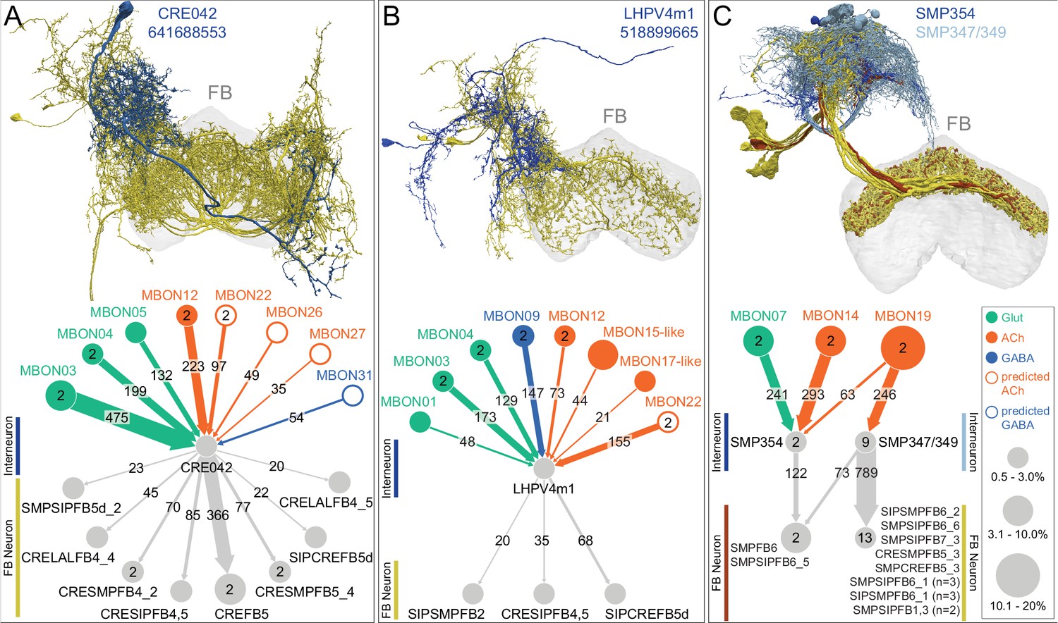
Examples of MBON to FB connectivity involving an interneuron.
(A–C) Examples of connectivity patterns observed for connections of MBONs to the FB through an interneuron. At the top of each panel the morphologies of the interneuron (blue) and FB neurons (yellow/brown) are shown. At the bottom of each panel a connectivity diagram is shown, with neurotransmitters color-coded and the size of the circles for MBONs representing the percentage of their outputs that goes to the shown interneurons. For FB neurons, the size of the circle represents the percentage of their inputs that comes from those interneurons. Note that interneurons in this pathway are often targets of multiple MBONs with neurotransmitters of opposite sign, a so-called ‘push-pull’ arrangement. (A) An interneuron, CRE042, that is strongly connected to MBONs of different valence inputs onto FB neurons of layers 4 and 5: CRESMPFB4_2 (FB4D), CRELALFB4_4 (FB4H), CRESIPFB4,5 (FB4X), SMPFB5 (FB5K), CRESMPFB5_4 (FB5L), CRELALFB4_5 (FB4J), SMPSIPFB5d_2 (FB5Y), and SIPCREFB5d (FB5AB) (see Figure 20—video 2). (B) An interneuron, LHPV4m1, that receives input from six MBON types and connects to three FB neurons of layers 2, 4 and 5: SIPSMPFB2 (FB2F_a), CRESIPFB4,5 (FB4X), and SIPCREFB5d (FB5AB). No other interneuron connecting to the FB gets input from more different MBONs (see Figure 29—video 3). (C) This interneuron can be divided into subtypes based on connectivity to α lobe MBONs: SMP347, SMP349, and SMP354, all of which are downstream targets of MBON19 (α2p3p), which conveys visual information (Figure 15A), but SMP354 consisting of two cells also gets strong input from MBON07 (α1) and MBON14 (α3) in a ‘push-pull’ arrangement. All these interneurons convey information mostly to: SMPSIPFB1,3 (FB1A), CRESMPFB5_3 (FB5H), SMPCREFB5_3 (FB5I), SMPSIPFB6_1 (FB6A), SIPSMPFB6_1 (FB6C_a, FB6C_b), SMPFB6 (FB6D), SIPSMPFB6_2 (FB6E), SMPSIPFB6_5 (FB6I), SMPSIPFB6_6 (FB6K), and SMPSIPFB7_3 (FB7F) (see Figure 20—video 4). Note these FB neurons contain 7 of the 9 cells in cluster 31 of Figure 34A.
Figure 20—video 1
MBONs providing direct input to the FB.
Figure 20—video 2
Multiple MBONs converge on an interneuron that provides input to the FB – example 1.
Figure 20—video 3
Multiple MBONs converge on an interneuron that provides input to the FB – example 2.
Figure 20—video 4
Multiple MBONs converge on an interneuron that provides input to the FB – example 3.
Figure 21 with 2 supplements
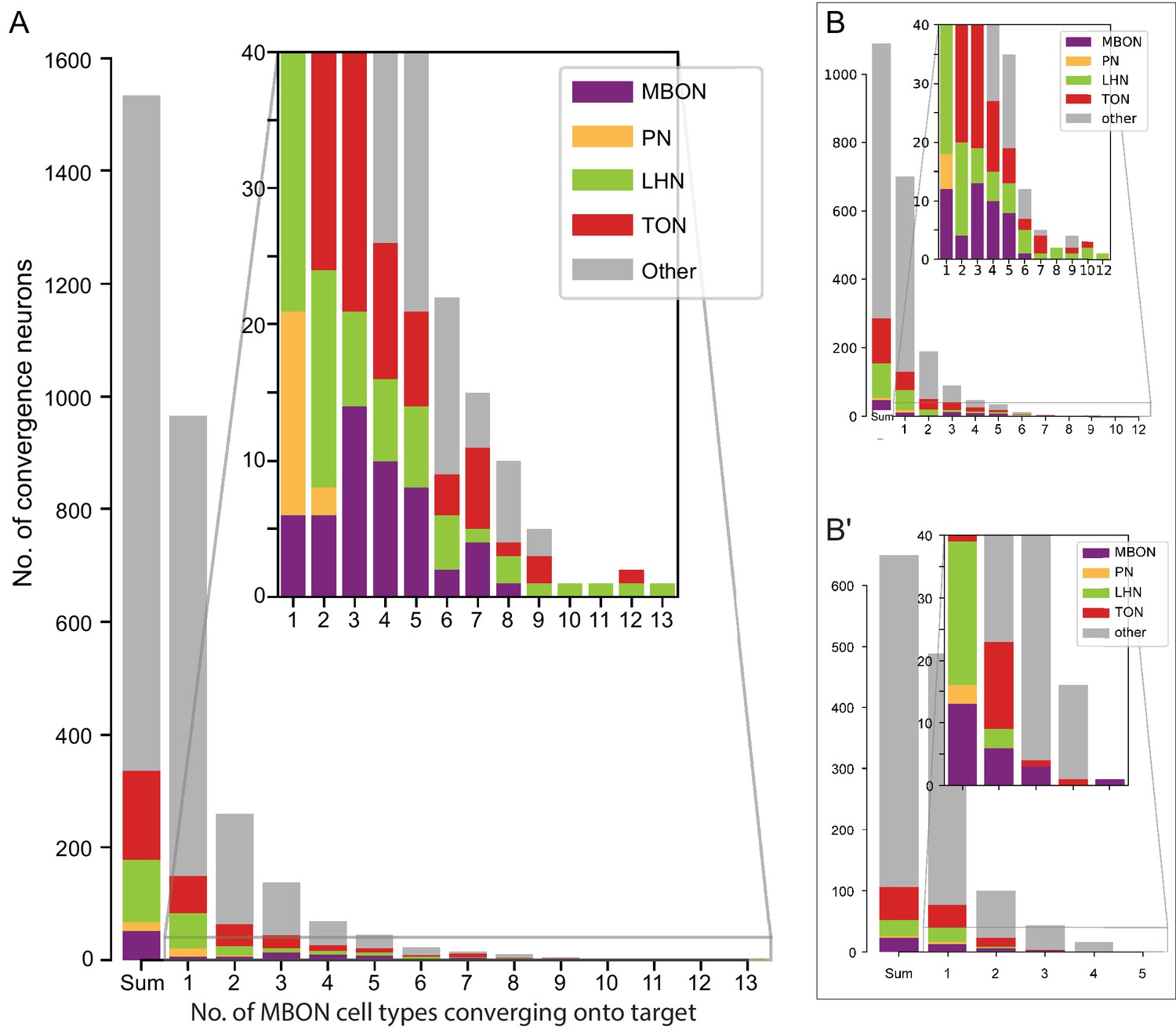
Downstream targets of MBONs often receive input from more than one MBON.
(A) About 1550 neurons are downstream (including axo-axonal connections) of one or more of the 34 MBON cell types when a threshold of 10 synapses is used. Among them, about 600 are downstream of at least 2 MBON cell types and are therefore capable of integrating information from multiple MBONs. The inset shows an expanded view of the indicated portion of the plot. These neurons include a range of well-characterized neuron types, including MBONs, olfactory projection neurons (PNs), lateral horn neurons (LHNs), and third-order olfactory neurons (TONs; downstream targets of PNs outside the LH, see Schlegel et al., 2020) as well as less characterized neurons (other). Among the neurons that receive input from 10 or more MBON types, LHNs are heavily over-represented. (B-B′) The distribution shown in (A) has been divided into two separate histograms, one showing neurons downstream of multiple typical MBONs, in which atypical MBONs have not been counted (B), and one showing neurons downstream of multiple atypical MBONs, in which typical MBONs have not been counted (B′). The insets show expanded views of the indicated portions of each plot. Atypical MBONs show less convergence than the typical MBONs and do not preferentially converge onto LHNs.
Figure 21—figure supplement 1
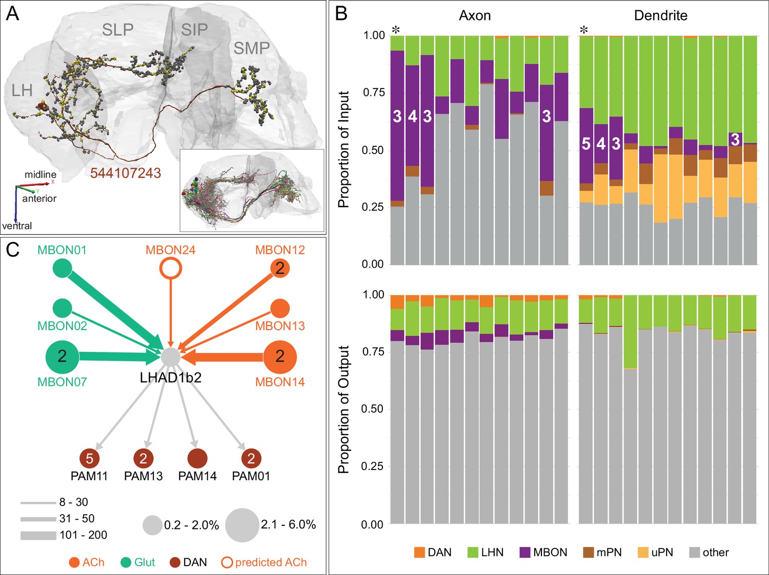
A LH neuron downstream of seven MBON types.
The previously reported LH output neuronal type (LHAD1b2; Dolan et al., 2019) acts as a site of integration of innate and learned information. (A) The morphology of a LHAD1b2_d neuron (544107243) is shown in maroon, with its presynaptic and postsynaptic sites represented by yellow and gray dots, respectively. The inset shows the morphologies of all twelve neurons of this cell type: LHAD1b2_a: 673426956 and 544107335; LHAD1b2_b: 5813022459, 573683438 and 483017681; LHAD1b2_c: 5813052205, 543321179, and 574040939; LHAD1b2_d: 544107243 and 730562988; LHAD1c1 : 729867599; and LHAD1c2 : 551298257. (B) Histograms of the proportion of inputs to (top) and outputs from (bottom) each of the twelve LHAD1 neurons from various classes of cells are shown, color-coded. These connections are divided into two groups based on the positions on the neurons’ arbors where they occur, labeled as Axon and Dendrite, based on the distribution of pre- and postsynaptic sites although all its arbors are mixed; the neuron order is the same in all histograms. The number of different MBON types innervating individual LHAD1 neurons varies; the number of MBON types providing input is indicated for those receiving input from three or more types. The neuron (544107243) shown in (A) and (C) is marked with an asterisk. (C) A connectivity diagram of the LHAD1b2_d neuron displayed in (A) is shown. This neuron receives input from seven MBON types and its downstream targets include four DAN cell types. The transmitters used by the MBONs are color-coded, the thickness of the arrows reflects synapse number, and the sizes of the circles that represent the MBONs reflects the percentage of their output directed to this LHAD1b2_d cell. The size of the circle representing LHAD1b2_d indicates the proportion of its total input that is derived from MBONs and the size of the circles representing the DANs indicate the fraction of their input provided by the LHAD1b2_d cell.
Figure 21—figure supplement 2
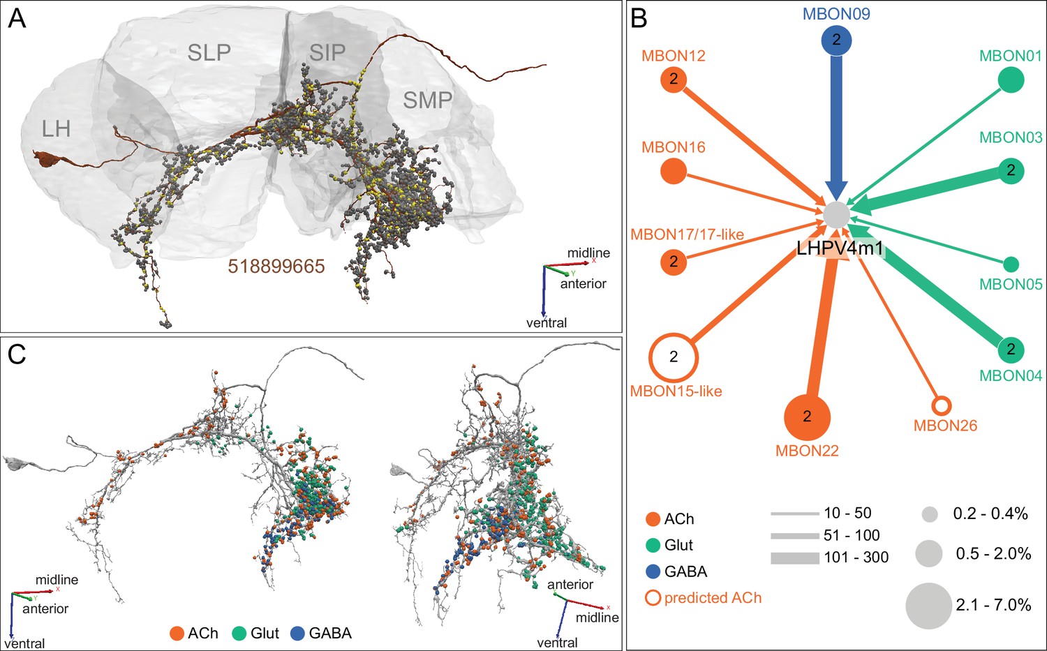
A neuron downstream of 11 MBON types.
This neuron LHPV4m1 (518899665) provides an extreme example of a neuron that integrates input from different MBON cell types. (A) The morphology of the neuron is shown in maroon, with its presynaptic and postsynaptic sites represented by yellow and gray dots, respectively. (B) Diagram showing the strengths of input from 11 different MBONs. The transmitters used by the MBONs are color-coded, the thickness of the arrows reflects synapse number, and the sizes of the circles that represent the MBONs reflect the percentage of their output directed to this neuron. (C) Distribution of sites of MBON input to the neuron, color-coded by MBON neurotransmitter type. Note that connections from MBONs with different neurotransmitters are segregated along the neuron’s different arbors; for example, cholinergic inputs are concentrated in its posterior branches.
Figure 22 with 4 supplements
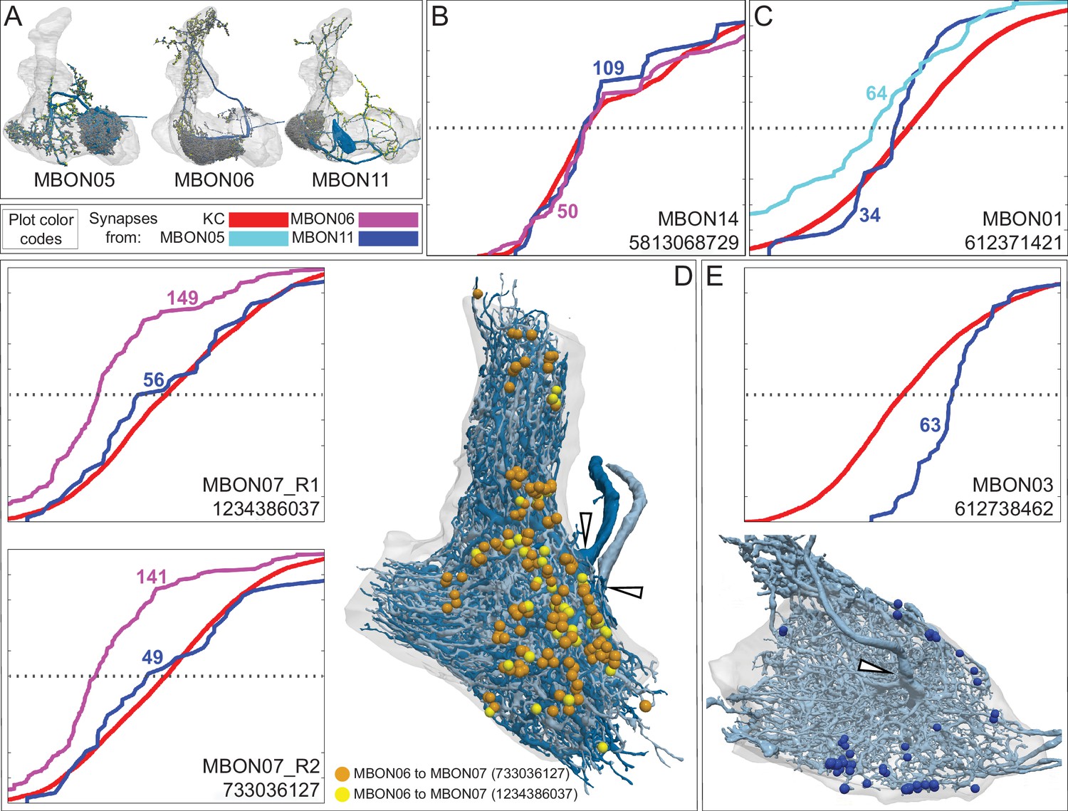
Spatial distribution of synapses from feedforward MBONs onto the dendrites of other MBONs.
(A) The three MBON types that make feedforward connections to other compartments within the MB lobes are shown. Neurons are shown in blue with presynaptic and postsynaptic sites shown as yellow and gray dots, respectively. (B–E) The cumulative fraction of synaptic connections from a feedforward MBON to its target is plotted as a function of the normalized distance from the root of the target MBON’s dendritic tree, on a linear scale from 0 to 1. The name of the target neuron is given in the lower right corner of the panel. The horizontal dotted line indicates the distance from the root of the target MBON’s dendritic tree at which half of the synapses from KCs to that MBON have occurred. The lines in these graphs are color-coded as indicated by key shown below panel A. The numbers indicate the total number of synapses between the neuron of the same color and the target MBON. (B) The synapses from MBON06 (β1>α) and MBON11 (γ1pedc>α/β) onto MBON14 in α3 have a similar spatial distribution as MBON14’s synapses from KCs, which tend to be uniformly distributed along MBON dendrites. (C) MBON01’s dendrites in γ5 receive synaptic connections from MBON11 closer to MBON01’s dendritic root than KC inputs, a bias even more pronounced in the distribution of synapses MBON01 (γ5β'2a) receives from MBON05 (γ4>γ1γ2). (D) The two MBON07 cells in the α1 compartment each receive synaptic input from MBON06 (β1>α) at sites close to the root of their dendrites (hollow arrowheads); in contrast, MBON11’s synapses onto the MBON07s have a similar distribution as the input the MBON07s receive from KCs. (E) MBON03 (β′2mp) receives synaptic input from MBON11 shifted further from its dendritic root (hollow arrowhead) than the input it receives from KCs.
Figure 22—figure supplement 1
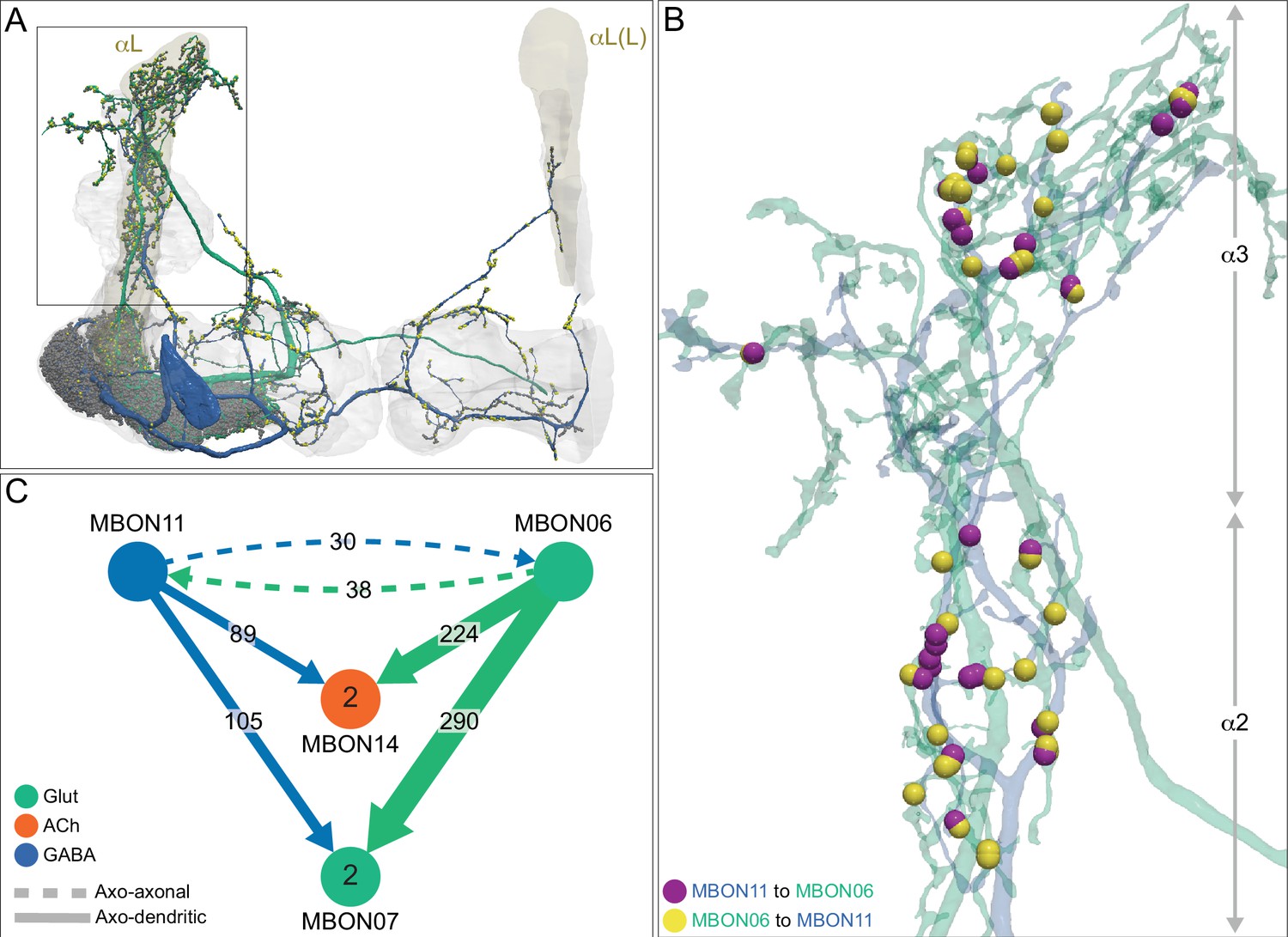
MBON06 and MBON11 make reciprocal axo-axonal connections in the α lobe.
(A) MBON06 (β1>α; green) and MBON11 (γ1pedc>α/β; blue) send axonal processes to the α2, α3 and, to a lesser extent, α1 compartments. (B) MBON06 and MBON11 make reciprocal axo-axonal connections, mostly in the α2 and α3 compartments. The positions of these synapses are shown, color-coded. (C) Diagram of a subset of connections involving MBON06 and MBON11, which both also make axo-dendritic connections onto MBON07 (α1) and MBON14 (α3) inside the MB lobes.
Figure 22—video 1
Feedforward MBON05.
Figure 22—video 2
Feedforward MBON06.
Figure 22—video 3
Feedforward MBON11.
Figure 23 with 3 supplements
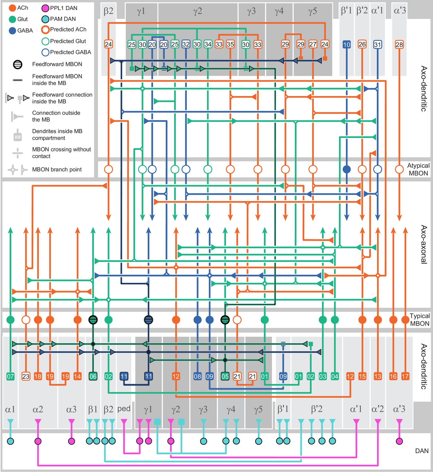
Diagram of the connections made between MBONs.
A diagram showing MBON-to-MBON connections. At the bottom, gray boxes representing each of the MB compartments and the core of the distal pedunculus (pedc). DAN inputs, with PPL1 and PAM DANs color-coded, are shown below the compartments (see Figure 6—figure supplement 1 for the names of these cell types). MBON dendrites are represented as squares that contain the identification number of the MBON cell type, color-coded by neurotransmitter; see Figure 7 for more information about these MBONs. At the top, gray boxes representing the subset of MB compartments that house the dendrites of atypical MBONs are shown; the identification numbers of the MBON cell types are given in the squares. These MBONs are described in more detail in Figure 8. Outputs from MBONs are shown outside the gray boxes, with the exception of three MBONs—MBON05 (γ4>γ1γ2), MBON06 (β1>α) and MBON11 (γ1pedc>α/β)—indicated by the heavier outline and striped circles representing their cell bodies, send axonal terminals (triangles) back into the MB lobes. These MBONs are described in more detail in Figure 22 and Figure 22—video 1, 2 and 3. Axo-dendritic and axo-axonal connections between MBONs are diagrammed separately, as indicated.
Figure 23—figure supplement 1
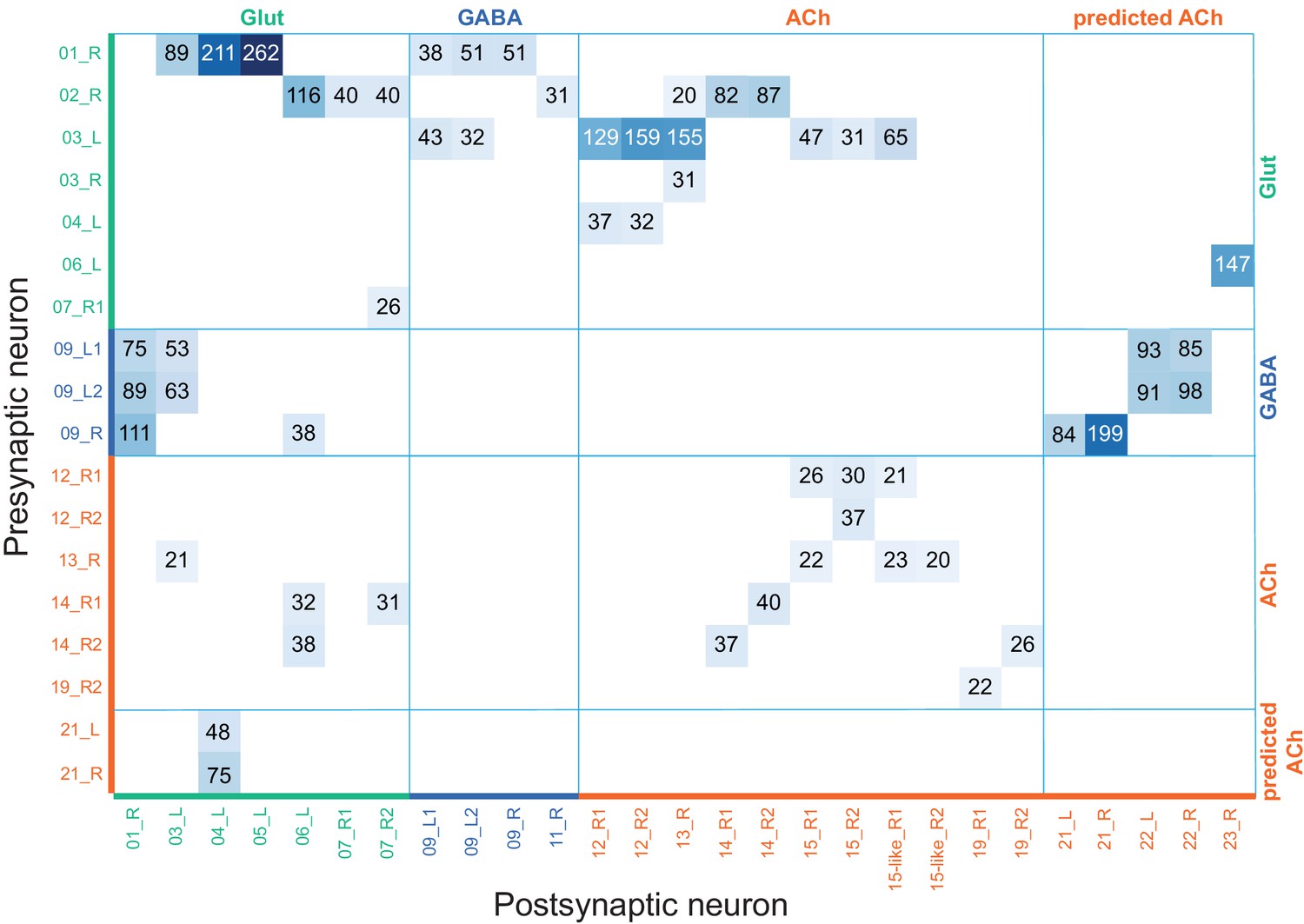
Axo-axonal connections among typical MBONs outside the MB presented as a connection matrix.
This matrix shows all axo-axonal connections between pairs of typical MBONs that involve 20 or more synapses. The MBONs on the vertical axis are presynaptic to those of the horizontal axis. MBON types are sorted by neurotransmitter. Blank rows or columns are not shown. Connections are seen more frequently and are stronger between glutamatergic MBONs onto cholinergic MBONs or other glutamatergic MBONs. Likewise, GABAergic MBONs frequently synapse onto the axons of glutamatergic MBONs and predicted cholinergic MBONs. In contrast, no axo-axonal synapses were seen between GABAergic MBONs or from cholinergic MBONs onto GABAergic MBONs. In several cases, axo-axonal synapses were highly localized and concentrated in a single axonal branch (see Figure 23—figure supplement 2).
Figure 23—figure supplement 2
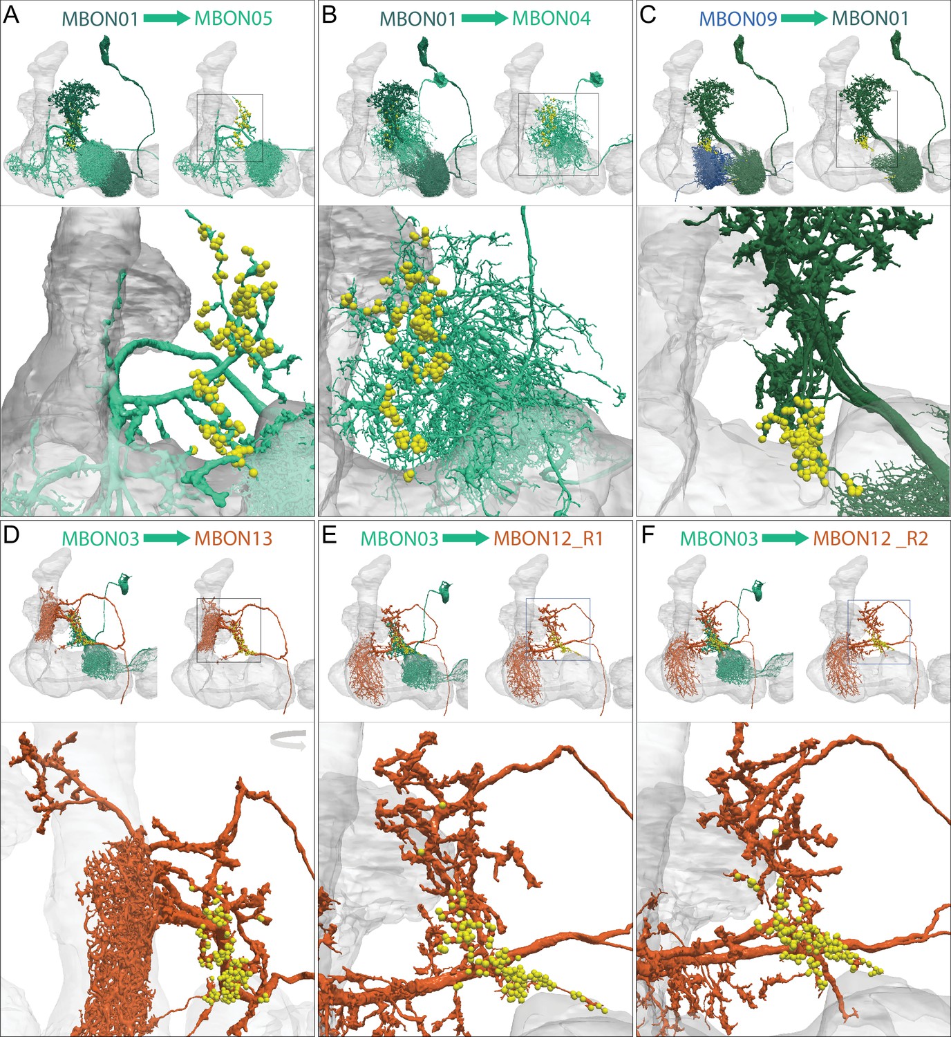
Axo-axonal synapses between MBONs can be highly localized.
(A–F) Each panel shows three images: a low magnification view (upper left) of two neurons that make axo-axonal connections, a low magnification view (upper right) of just the postsynaptic neuron, and a higher resolution view of the relevant portion of its axonal arbor (lower). Neurons are color-coded by neurotransmitter type. Synapses are depicted as yellow dots. (A–B) MBON01 (γ5β'2a; dark green) forms axo-axonal connections onto MBON04 (β′2mp_bilateral) and MBON05 (γ4>γ1γ2) with similar synapse counts, 211 and 262 respectively. (A) Synapses from MBON01 to MBON05 are widely distributed throughout MBON05’s axonal terminal. (B) Synapses from MBON01 to MBON04 are highly biased toward the lateral and anterior of MBON04’s axonal terminal. (C) MBON01 receives over 100 synapses from MBON09 (γ3β′1)_R onto its axon. Most of these connections are localized in a smaller branch that is ventral and isolated from its main axonal arbor. (D) Localized axo-axonal connections from MBON03 (β′2mp) to MBON13 (α′2). Note that the enlarged image has been rotated to improve visibility of the relevant arbor. (E–F) Localized axo-axonal connections between MBON03 and each of two MBON12 (γ2α′1) cells occur in the same location on the axonal arbors of MBON12-R1 (E) and MBON12-R2 (F).
Figure 23—figure supplement 3
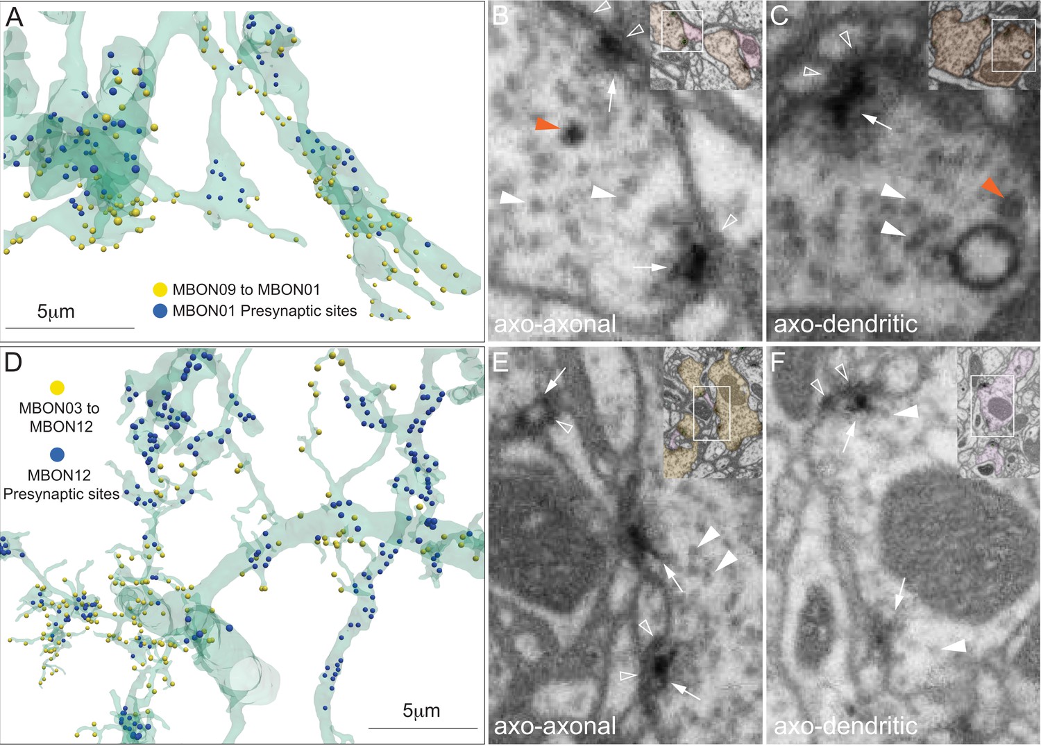
Morphology of axo-axonal synapses.
(A) A portion of the MBON01 (γ5β'2a) arbor from within the enlarged area shown in Figure 23—figure supplement 2C is shown in transparent green. The relative locations of axo-axonal synapses from MBON09 (γ3β′1) onto MBON01 (yellow dots) and MBON01’s output synapses to its downstream targets (blue dots) are indicated. (B) Electron micrograph from the hemibrain dataset showing two MBON09 to MBON01 axo-axonal synapses (white arrows). Two types of vesicles are indicated by the arrowhead (small clear vesicle, white arrowhead; larger dense core vesicle, orange arrowhead). Postsynaptic densities are indicated by the hollow white arrowheads. The inset in the upper right shows a lower magnification view; MBON09 is colored brown, MBON01 is pink and annotated presynaptic sites are marked by the small green circles. (C) An axo-dendritic synapse from MBON09 to one of its downstream targets is shown for comparison. The morphologies of MBON’s axo-axonal and axo-dendritic synapses are similar. (D) A portion of the MBON12 (γ2α′1) arbor from within the enlarged area shown in Figure 23—figure supplement 2F is shown in transparent green. The relative locations of axo-axonal synapses from MBON03 (β′2mp) onto MBON12 (yellow dots) and MBON12’s output synapses to its downstream targets (blue dots) are indicated. (E) Electron micrograph from the hemibrain dataset showing three MBON03 to MBON012 axo-axonal synapses (white arrows). Small clear vesicles are indicated by the white arrowheads. Postsynaptic densities are indicated by the hollow white arrowheads. The inset in the upper right shows a lower magnification view; MBON03 is shaded brown, MBON12 is pink. (F) An axo-dendritic synapse from MBON12 to one of its downstream targets is shown for comparison. The inset in the upper right shows a lower magnification view; MBON12 is shaded pink. The morphologies of MBON’s axo-axonal and axo-dendritic synapses are similar.
Figure 24 with 1 supplement
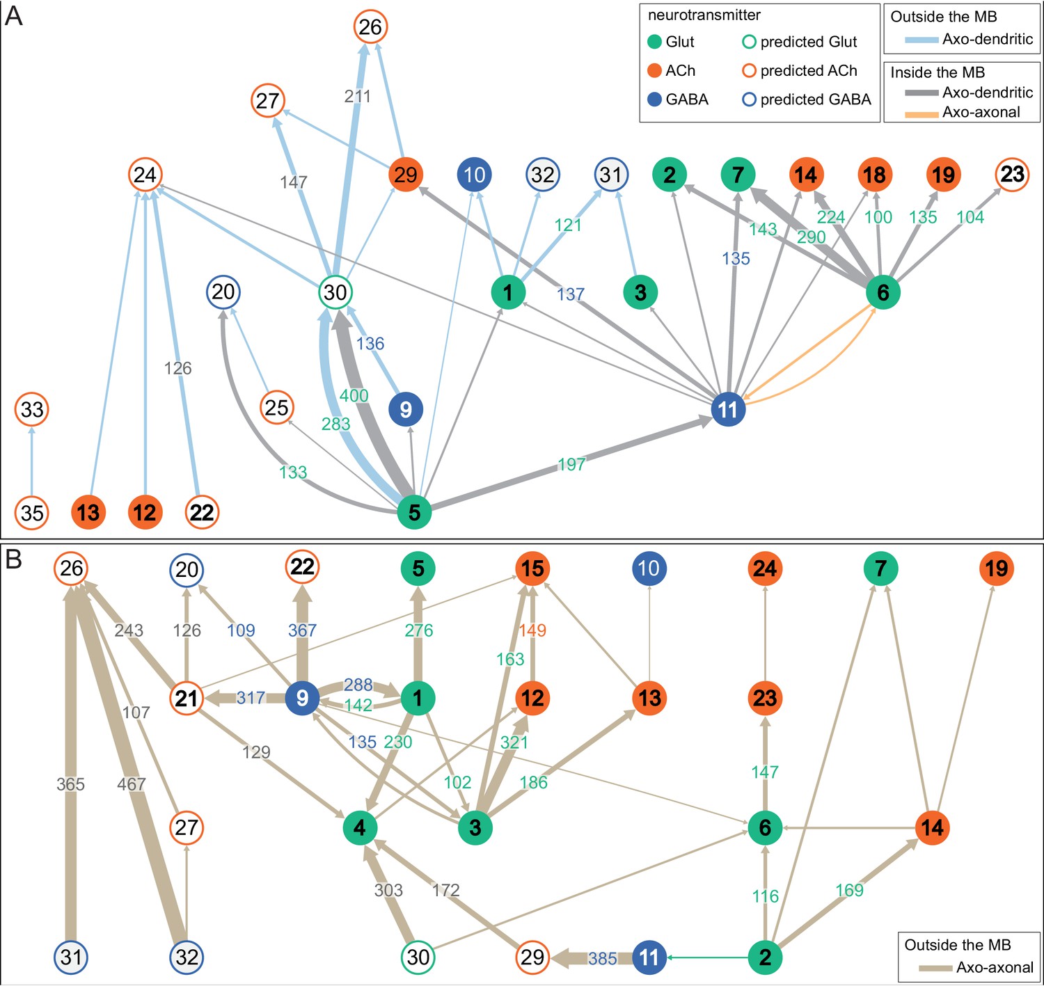
Connections between MBONs form a multi-layered feedforward network.
Connections between MBONs, including both typical and atypical MBONs are shown, using a threshold of 30 synapses. The color of the arrow, as indicated in the color key, represents the nature and location of the synaptic connection. The number of synapses made in any given connection is indicated by the number in the arrow and the arrow thickness is proportional to that number. Numbers have been pooled for cases where there are two MBONs of the same cell type but only connections that occur in the right hemisphere are shown. The numbers within the circles indicate the MBON cell type; for example 1 represents MBON01. Typical MBONs are numbered with bold numerals. Circles are color-coded according to their neurotransmitter. (A) Axo-dendritic connections outside the MB lobes, axo-dendritic connections inside the MB lobes provided by feedforward MBONs (MBON05, MBON06, and MBON11), and the reciprocal axo-axonal connections between MBON6 and MBON11 within the MB lobes. (B) Axo-axonal synapses outside the MB lobes. Note that some MBONs, such as MBON24, form both axo-dendritic and axo-axonal connections outside the MB. Additional details of MBON05’s innervation of MBON30 are provided in Figure 24—figure supplement 1A.
Figure 24—figure supplement 1
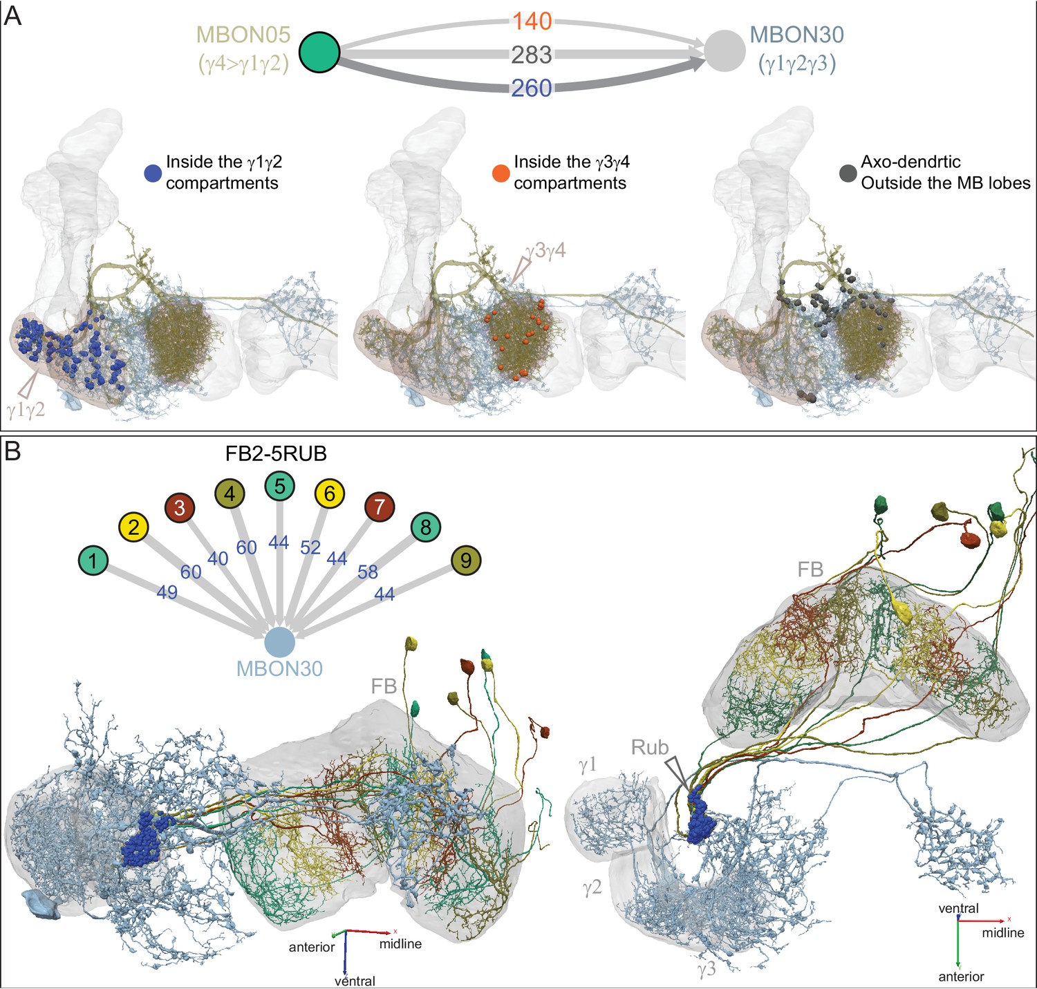
MBON30 displays an unusual pattern of innervation from other MBONs and FB neurons.
(A) MBON30 receives strong input from MBON05, a feedforward glutamatergic MBON, through three distinct axo-dendritic paths: inside the γ1 and γ2 compartments (260 synapses); inside the γ3 and γ4 compartments (140 synapses); and outside the MB lobes (283 synapses). The locations of synapses used in each of these three connections are shown. Note that in the connectivity diagram in Figure 24, the arrow represents all 400 synapses that occur in either the γ1 and γ2 compartments (260) or in the γ3 and γ4 compartments (140). (B) MBON30 receives strong input from the FB mediated by the FB2-5RUB cell type which has nine columnar cells. The connection occurs inside the RUB. MBON30 is the only MBON that has input from an FB cell type among its top 10 inputs.
Figure 25 with 2 supplements
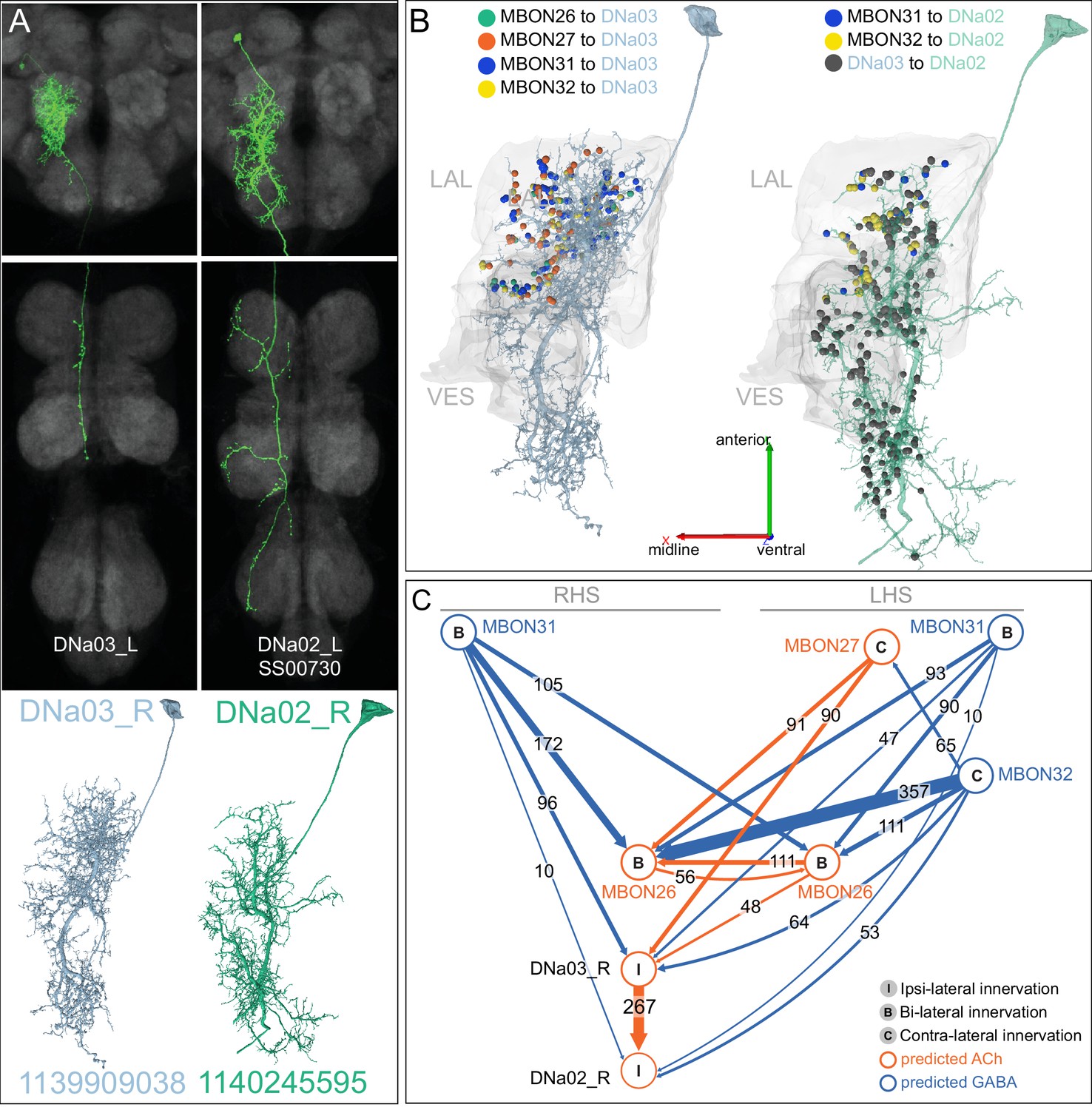
A descending pathway from atypical MBONs to the ventral nerve cord (VNC).
Four LAL-innervating atypical MBONs form strong connections to descending neurons (DN). (A) A comparison between LM (Namiki et al., 2018) and EM morphologies of DNa02 and DNa03. Note that the LM images show the cells in the left hemisphere while the EM images are from the right hemisphere and that the axons of the DNs extend outside the hemibrain volume. (B) Synaptic connections from MBON26, MBON27, MBON31 and MBON32 to DNa03 (left) and from MBON31, MBON32, and DNa03 to DNa02 (right) are shown, color-coded. Note the connections from MBONs are restricted to the LAL while DNa03 makes synapses onto DNa02 throughout its arbor in the LAL and the VES. (C) Diagram of connectivity between MBONs, DNa03 and DNa02. Note that MBON27 and MBON32 have contralateral axons (Figure 8—figure supplements 6 and 11, Figure 8—video 6 and 11) and thus innervate the contralateral DNa02 and DNa03 while MBON26 and MBON31 have bilateral output (Figure 8—figure supplements 5 and 10, Figure 8—video 5 and 10). Thus the connectivity diagram shows the inputs onto the DNa02 and DNa03 of the right hemisphere (RHS), while many of the neurons providing input have their cell bodies in the left hemisphere (LHS). MBONs 26, 31, and 32 show similarity in their PN inputs and overall outputs (see Figure 16—figure supplement 2). Other inputs to DNa02 and DNa03 are summarized in Figure 25—figure supplement 1. Predicted neurotransmitters are indicated. In addition to the diagrammed connections, these MBONs connect to the DNa02 and DNa03 using paths that include interneurons (see Figure 42). DNa02 has been implicated in steering control (Rayshubskiy et al., 2020) and the outputs of these MBONs are likely to play a role in guiding approach and avoidance (see Figure 42).
Figure 25—figure supplement 1
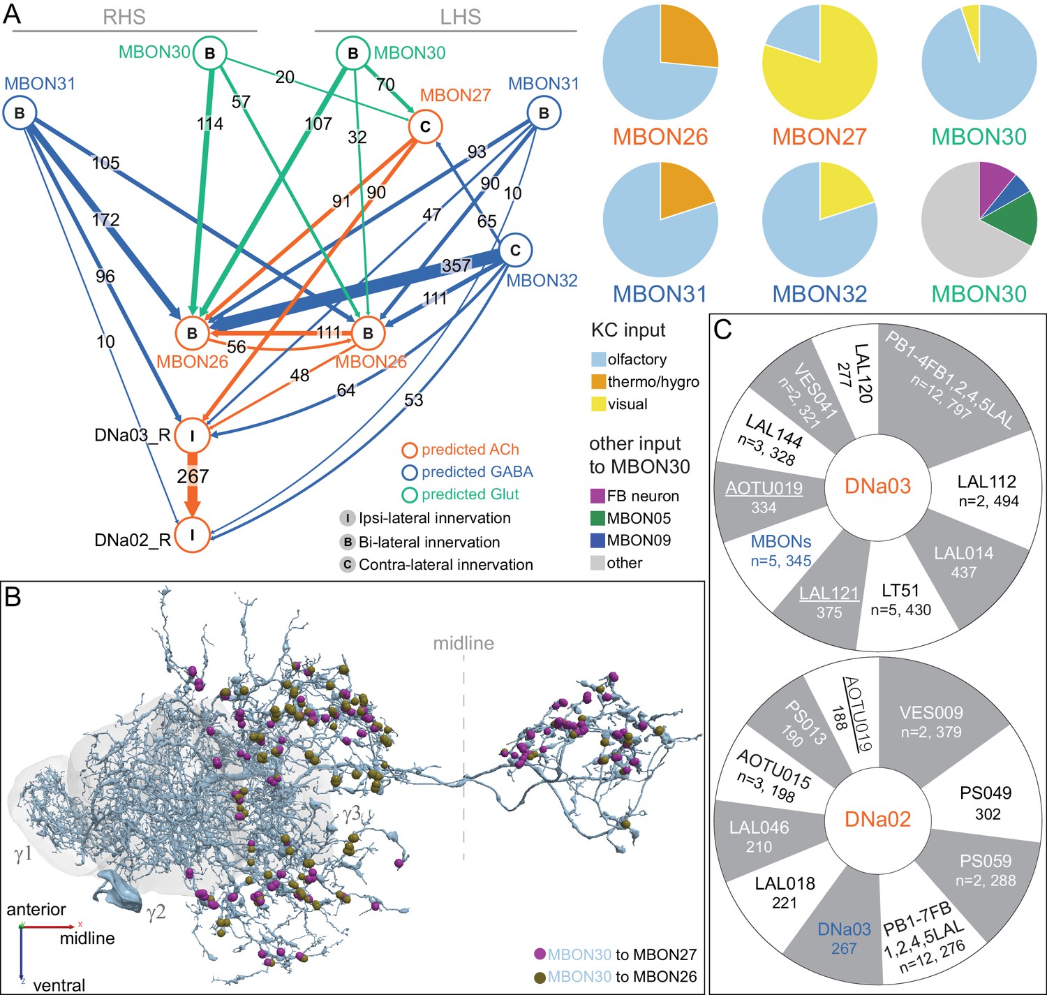
Top inputs to DNa02 and DNa03.
(A) Left: Expanded connectivity diagram now including MBON30. MBON30 provides strong input to MBON26 and MBON27 (Figure 24) and conveys information from the FB (Figure 24—figure supplement 1B; Figure 8—video 9). Right: Pie charts describing inputs to MBON26, MBON27, MBON30, MBON31 and MBON32. The first five pie charts show the modalities of sensory information conveyed to these MBONs by KCs (data taken from Figure 15—figure supplement 2). Note MBON26 and MBON31 receive substantial thermo/hygrosensory input and MBON 27 and MBON32 receive substantial visual input. As shown in the sixth pie chart, MBON30 receives strong input from MBON05 and MBON09, as well as from a single FB columnar neuron cell type (FB2-5RUB); these three cell types provide 36% of MBON30’s input, when input from KCs, DANs, APL, and DPM is excluded. (B) The presynaptic sites on MBON30 that connect to MBON26 and MBON27 are shown, color-coded. (C) Sunburst charts showing the 10 cell types providing the largest amount of input, based on synapse number, to DNa03 (top) and DNa02 (bottom). The number of synapses and the number of cells in the cell type if more than one (n=) are shown. Predicted neurotransmitter types are indicated.
Figure 25—figure supplement 2
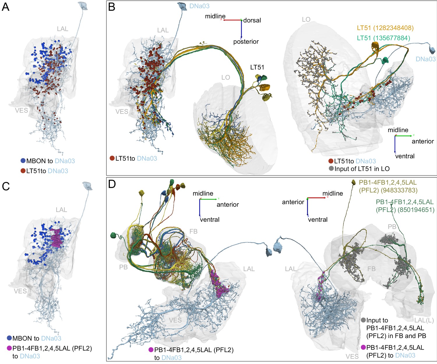
Central complex and LO inputs to DNa03.
(A) DNa03 receives strong visual input from lobula tangential (LT) neurons, LT51 (also see Figure 25—figure supplement 1C). The five LT51 neurons make 430 synapses onto DNa03, shown as reddish brown dots. These connections are located at the core of the DNa03 dendrite while the MBONs synapse onto DNa03 around the periphery (shown as blue dots). The five LT51s that synapse onto DNa03 represent only a subset of the twelve LT51 identified in the right optic lobe and the two of these cells account for 362 of the 430 synapses from LT51 cells to DNa03. Interestingly, these five connected LT51 cells have their dendrites in the same half of the lobula, corresponding to the frontal part of the visual field. (B) Left: a dorsal view of LT51 connecting to DNa03. Right: two LT51 neurons connecting to DNa03 are shown with their postsynaptic sites in the LO indicated by the gray dots and presynaptic connections to DNa03 as reddish brown dots. (C) The strongest input cell type to DNa03 is a cell type with dendrites in the PB and the FB, PB1-4FB1,2,4,5LAL(PFL2), with 12 such cells making a total of ~800 synapses (also see Figure 25—figure supplement 1C). These synaptic connections are highly concentrated on a small dendritic area of DNa03, shown in purple with MBON input on the periphery (blue). (D) Left: Side view of the connections between the PFL2 neurons and DNa03. Right: Two of the PFL2 neurons are shown with their output to DNa03 (purple) and their input sites in FB and PB (gray). Note that PFL2 neurons are highly polarized.
Figure 26 with 3 supplements

Feedback from MBONs to DANs.
Input from MBONs onto DANs occurs in three distinct circuit motifs which are diagrammed. MBON connections to DANs from the same compartment are depicted as a yellow arrow, while MBON connections to DANs from a different compartment are depicted as a purple arrow. DANs downstream of these MBONs are depicted as dashed yellow arrows. (A) In the simplest case, the MBON and DAN form a reciprocal loop where the MBON innervates DAN(s) that send their axons back to the same compartment where the MBON’s dendrites arborize. Below the diagram of this circuit motif, each of the instances we observed with this arrangement is presented; inputs onto PAM and PPL1 DANs are presented separately. The color of the MBON name indicates its neurotransmitter, as indicated. (B) In this case, MBON(s) synapse onto DAN(s) that send their axons to MB compartment(s) different from the compartment where the MBON’s dendrites reside, providing a mechanism for cross-compartment communication. It is common for the DAN population of a compartment to receive input from several MBONs. (C) This motif combines the previous two motifs, with DANs receiving input from both MBON(s) of same and different compartments. (D) The table summarizes DAN populations that participate in the three different feedback motifs.
Figure 26—figure supplement 1
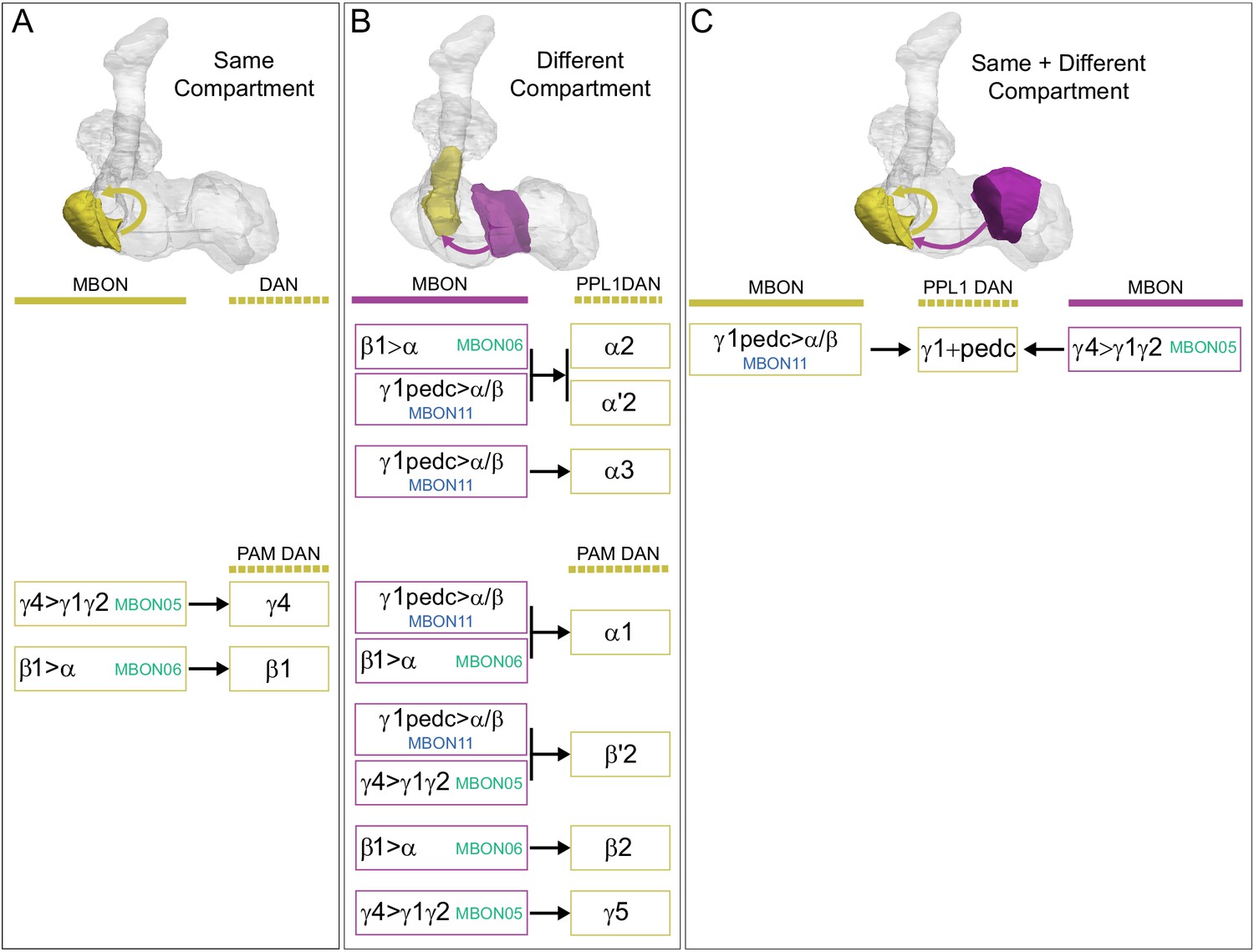
Axo-axonal connections from MBON05, MBON06 and MBON11 onto DANs inside MB lobes.
These three MBONs send axonal processes to other MB compartments (Aso et al., 2014a) where they make synapses onto other MBONs (see Figure 22 and Figure 22—figure supplement 1). As summarized here, they also make axo-axonal synapses onto DANs in the same compartments where they contact other MBONs. In some other compartments, they make a smaller number of synapses onto DANs. For example, MBON06 (β1>α) and MBON11 (γ1pedc>α/β) make a total of 279 synapses onto the axons of two PPL1 and six PAM DANs in the α lobe and 53 synapses onto six PAMs in the β′2, β2, and β1 compartments. Similary, MBON05 (γ4>γ1γ2) makes a total of 156 synapses onto one PPL1 and five PAM DANs in the γ1 and γ2 compartments and a total of 10 synapes onto two PAM DANs in other compartments. Presynapses of MBON11 in the β′2 compartment were also observed in the FAFB EM volume by Felsenberg et al., 2018. It is worth noting that these connections represent a much smaller fraction of the total inputs that DANs receive within the MB lobes when compared with percentage of inputs provided by the MBON feedback that goes to DAN dendrites shown in Figure 26. (A) MBON05 and MBON06 feedforward to the axons of PAMs from the same compartments. (B) Feedforward connections from MBON06 and MBON11 to PPL1 and PAM DANs in other compartments. The connections in the β′2, β2, and γ5 compartments are weaker than those in the α-lobe. (C) The PPL101 (γ1-pedc) DAN receives feedback from both MBON11 (same compartment) and MBON05 (other compartment).
Figure 26—figure supplement 2
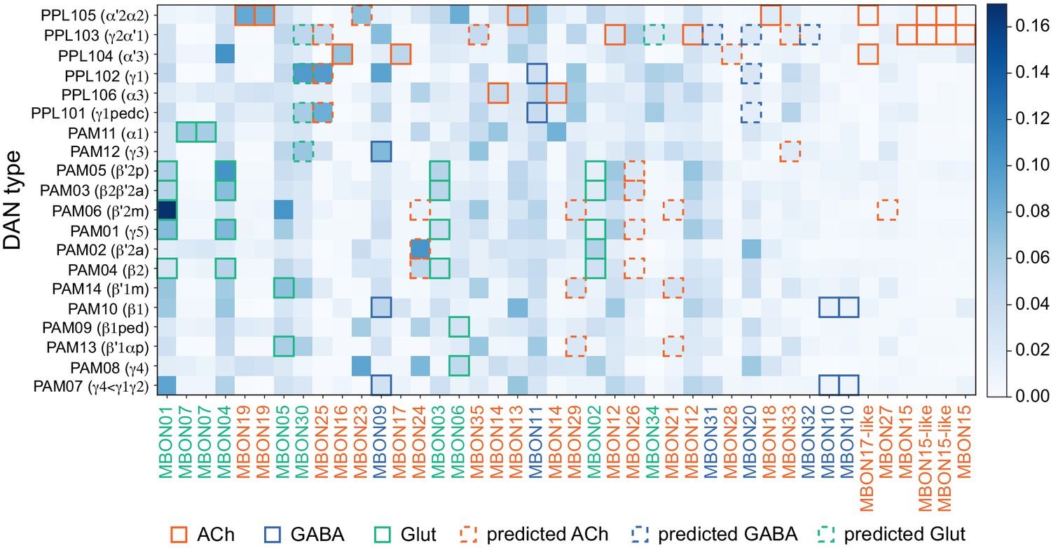
MBON-to-DAN feedback mediated by an interneuron.
MBONs also make indirect connections to DANs in which the MBON connects to an interneuron which then connects to a DAN. This matrix shows the effective connection strength of such MBON-to-DAN feedback loops and is meant to complement the data presented in Figure 26, which describes direct connections between MBONs and DANs. Effective connection strength is a measure that takes into account both the strength of the MBON’s connection to the interneuron and that of the interneuron to the DAN. Effective connection strength is computed by multiplying the matrix of DAN inputs with the matrix of MBON outputs (both matrices are normalized so that the inputs to each neuron sum to 1). This connection strength is averaged across all DANs of the indicated type. Highlighted boxes indicate interactions between MBONs and DANs that share a compartment, and the box color indicates the neurotransmitter or predicted neurotransmitter of the MBON. MBONs are ordered by their proportion of self-feedback, as defined and shown in Figure 26—figure supplement 3.
Figure 26—figure supplement 3
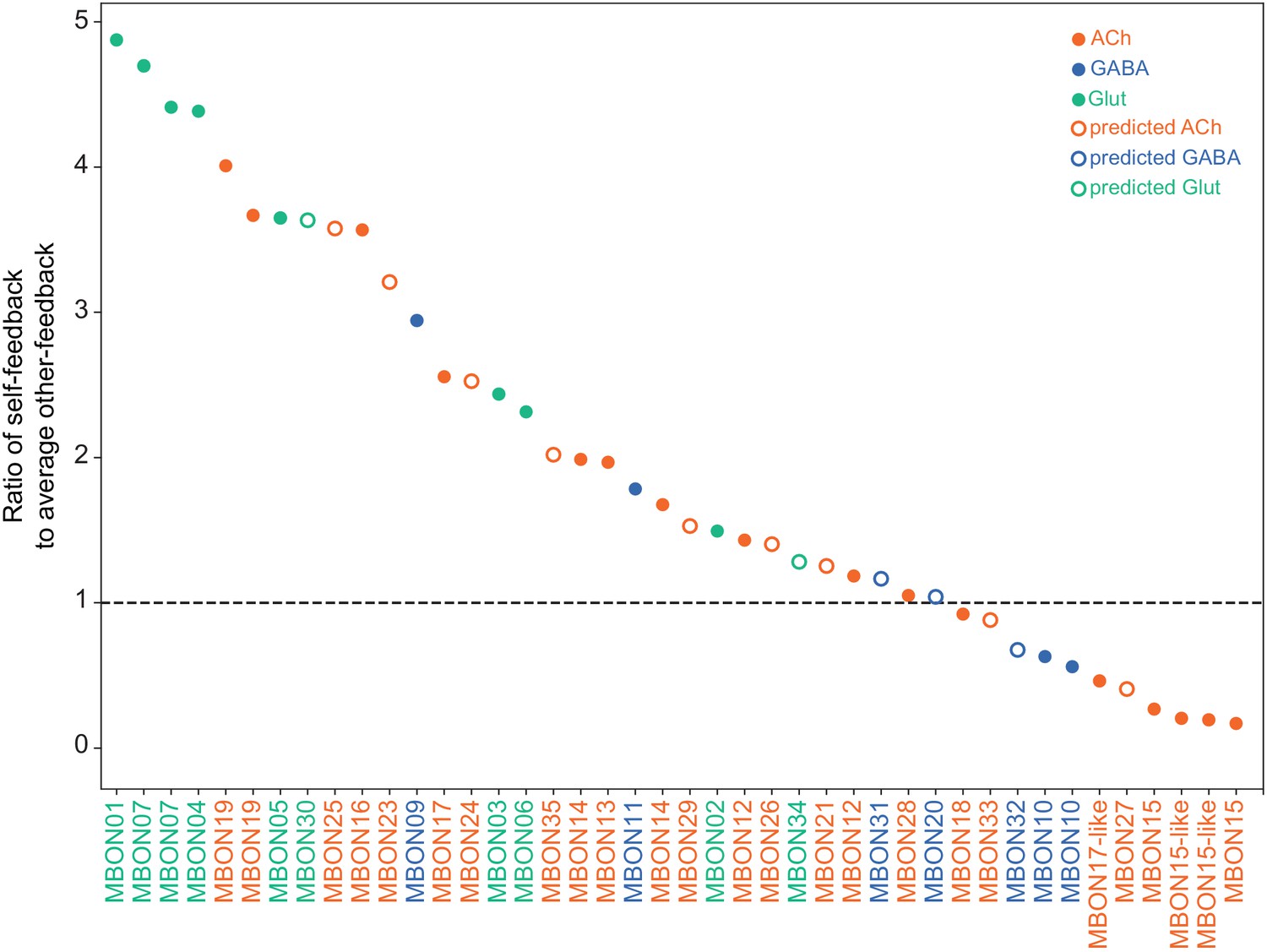
Distribution of DAN feedback mediated by an interneuron.
This plot shows the ratio of feedback to the same compartment (self-feedback) to feedback to other compartments (other-feedback) for each MBON type. Circles are color-coded to indicate the MBON neurotransmitter. The plot reveals a robust pattern of glutamatergic MBONs indirectly modulating their associated DANs. The plot is meant to complement the data presented in Figure 26, which describes direct connections between MBONs and DANs. The strength of indirect self-feedback is defined as the average effective connection strength mediated by one interneuron between a given MBON and the DANs that innervate the same compartment. The strength of average other-feedback is defined as the average effective connection strength between the MBON and all other DANs, again mediated by one interneuron. The value plotted on the y-axis is the ratio of these two quantities. That is, MBONs with higher ratios have a larger fraction of the interneuron-mediated feedback they initiate directed back to their own compartment, rather than to other compartments.
Figure 27 with 4 supplements
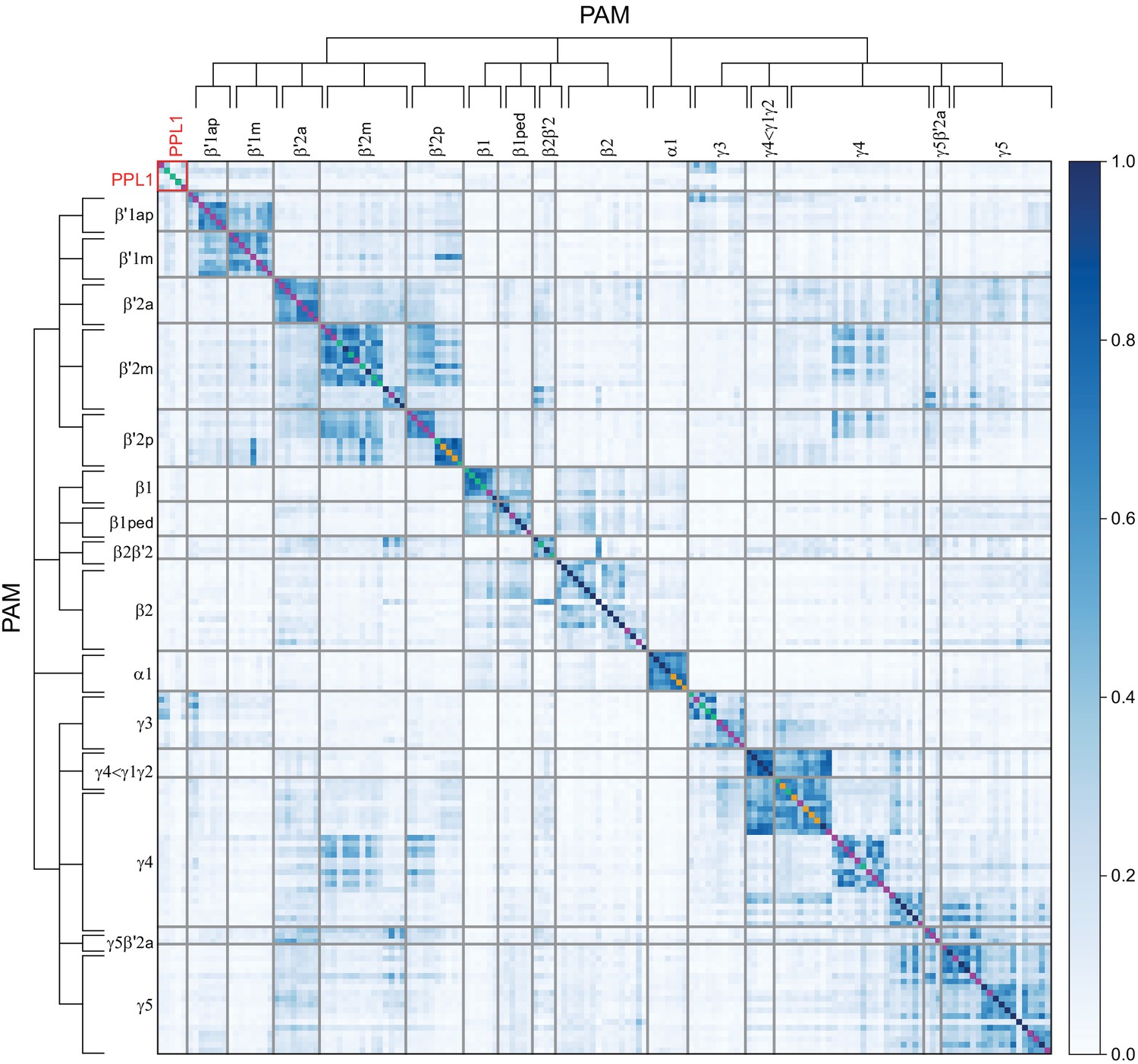
Similarity of input to individual DANs.
Heatmap representing the similarity of inputs received by DANs. Each square represents the cosine similarity of inputs received by each PAM or PPL1 DAN. In order to focus on inputs received outside the lobes of the MB, inputs from KCs, other DANs, APL, and DPM neurons have been excluded. DANs are grouped by type, and the ordering within each type is determined by spectral clustering. Colors on the diagonal indicate whether the given DAN receives feedback from MBONs in the same compartment (yellow), MBONs from different compartments (purple), both (green), or neither (dark blue) as defined in Figure 26. Figure 27—figure supplement 1 shows an expanded view of the PPL1 DAN portion of the heatmap. Figure 27—figure supplement 2 shows the average input similarity between DAN cell types computed after pooling the data for all cells of a given DAN cell type.
Figure 27—figure supplement 1
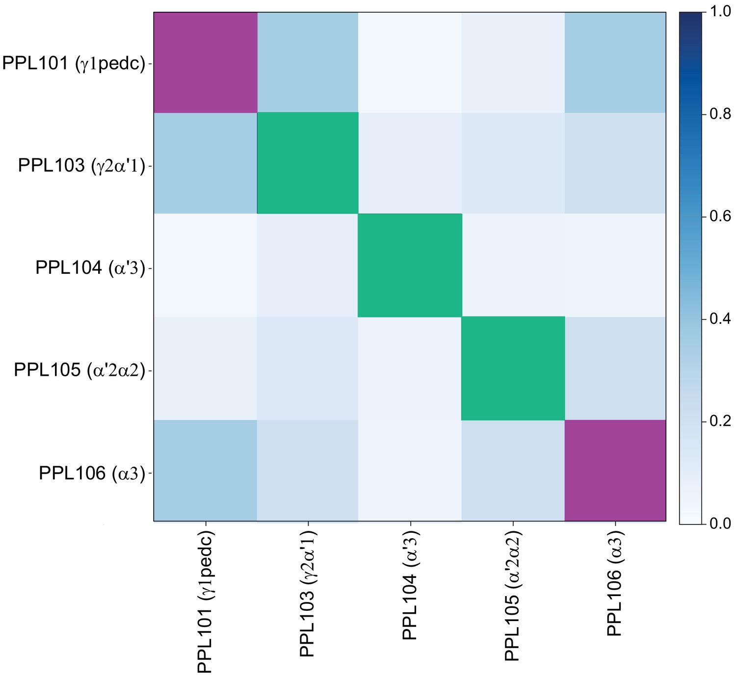
Similarity of inputs to PPL1 DANs.
Expanded view of Figure 27 for PPL1 DANs (red square in Figure 27). Note that each PPL1 DAN receives direct feedback from MBONs. Colors on the diagonal indicate whether the given DAN receives feedback from MBONs in a different compartment (purple) or from both the same and different compartments (green).
Figure 27—figure supplement 2
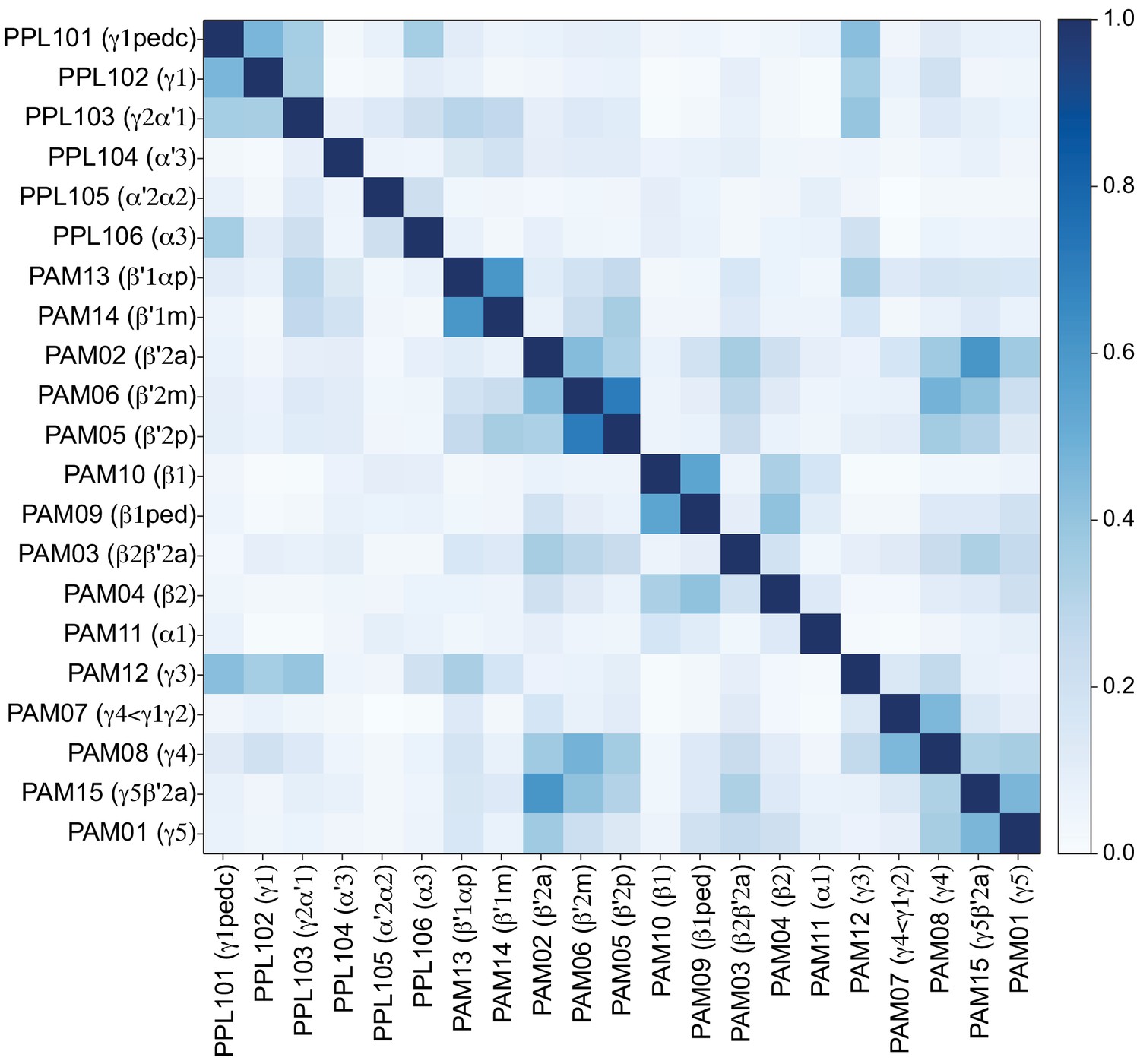
Similarity of inputs to DAN cell types.
Average input similarity between DAN cell types computed after pooling the data for all cells of a given type, as compared to Figure 27 where each individual DAN is plotted separately.
Figure 27—figure supplement 3
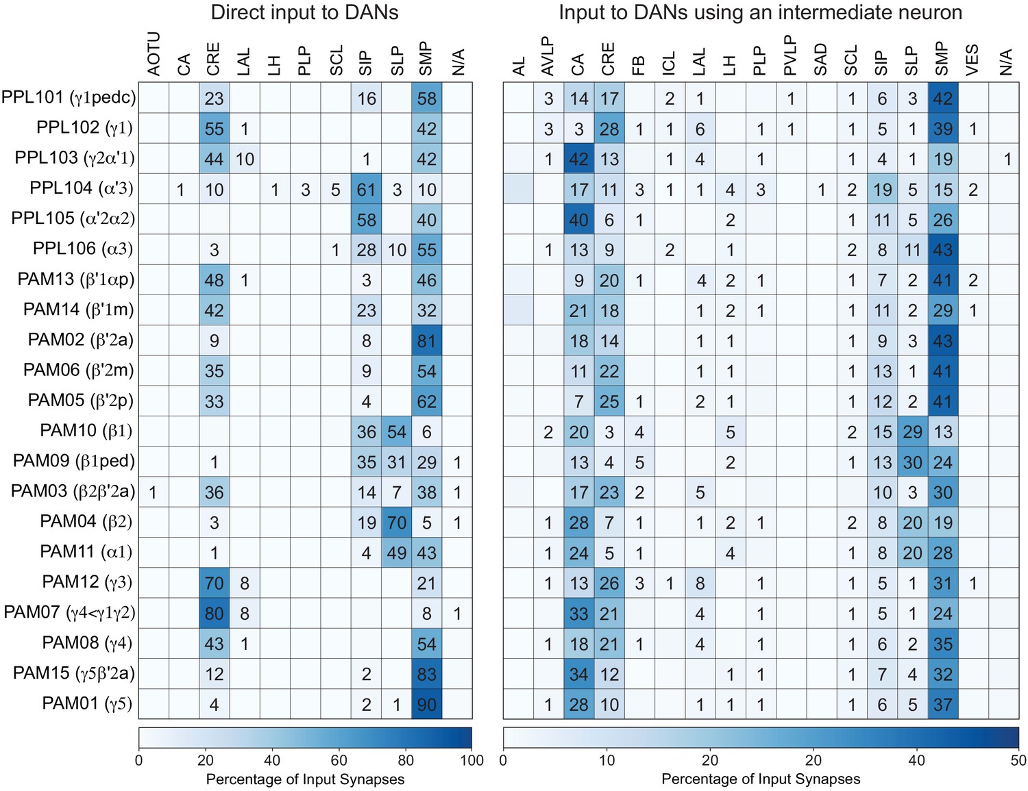
DAN input distribution by brain region.
(Left) The value in each box indicates the percentage of the given DAN type’s input synapses that lie in the given brain region. Blank boxes indicate values of less than 1%. (Right) Distribution of brain regions providing input to DAN types using an intermediate interneuron. The value in each box indicates the effective input to the given DAN from the given brain region, mediated by one interneuron. Effective input is a measure that takes into account both the strength of the connection of each of the neurons that provide input to the DAN and the connection strength of other neurons to each of those input interneurons in each brain region. Effective input is computed by matrix-multiplying the inputs to the DANs and the inputs to those DAN-presynaptic neurons (normalizing both matrices so that inputs to all neurons sum to 1). Blank boxes indicate values of less than 1%. The two distributions are generally similar, but there are some clear differences. For example, direct input from CA is minimal but very prominent in input mediated by an interneuron; for example, the γ2α'1 PPL103 DAN receives over 40% of its indirect input from the CA.
Figure 27—figure supplement 4
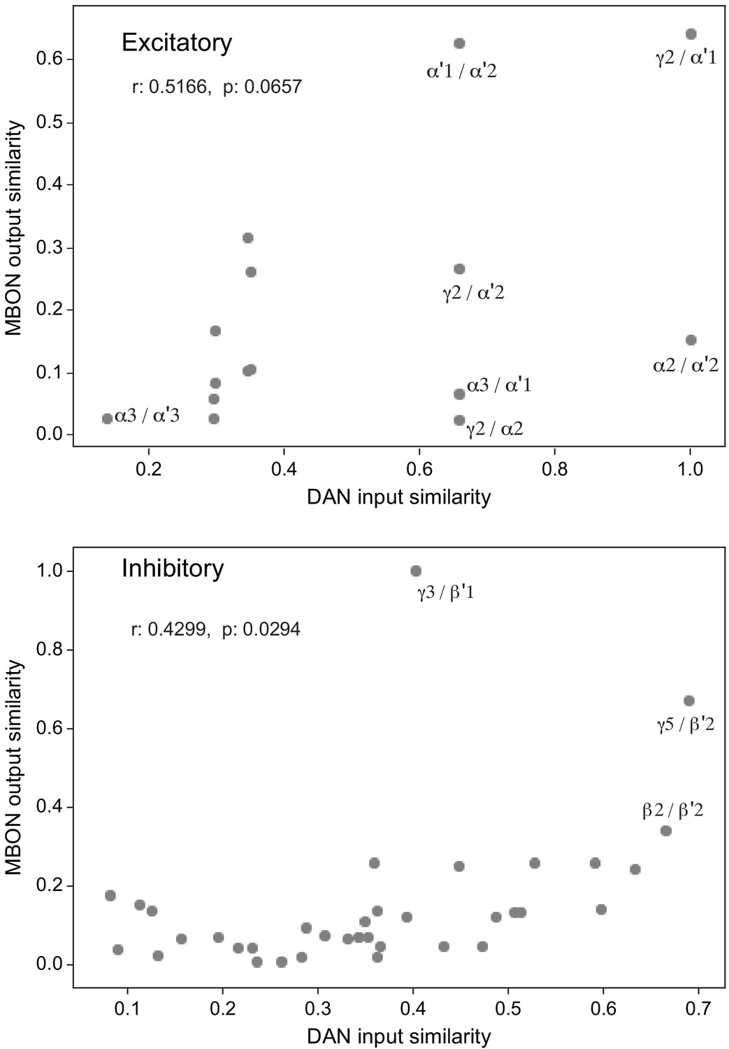
Comparing DAN inputs and MBON outputs reveals credit assignment by DANs.
Scatter plot of DAN input similarity (data from Figure 27) and MBON output similarity (data from Figure 16, collapsed by compartment). Each point represents a pair of compartments; notable pairs are labeled in the figure. DAN input similarity is defined as the cosine similarity of the inputs to the DANs of two compartments. MBON output similarly measures the cosine similarity of the outputs from the MBONs in those compartments. The relationship between the two similarity measures indicates that compartments whose MBONs project to similar downstream targets have DANs that receive similar inputs. This structure suggests a form of ‘credit assignment’ in which compartments whose MBONs control similar behaviors also receive similar reinforcement signals. Results are shown for compartments whose MBONs express excitatory (top, ACh) or putatively inhibitory (bottom, GABA, and Glu) neurotransmitters.
Figure 28 with 1 supplement
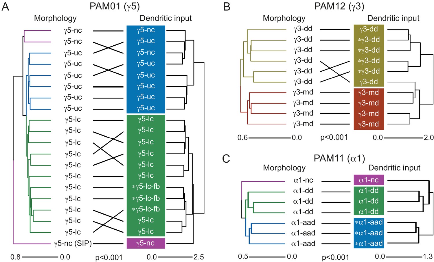
Morphologically defined DAN subtypes receive similar input.
Tanglegrams show that DAN subtyping based on hierarchical morphological clustering matches that generated by hierarchical clustering by input connectivity (compare this figure to DAN input similarity shown in Figure 27). We show data here for three compartments; we found that clustering by morphology or input connectivity gave similar results in all PAM DAN compartments (not shown). A complete list of PAM subtypes is given in Supplementary file 1. (A–C) Tanglegrams for right hemisphere PAM01 (γ5), PAM12 (γ3), and PAM11 (α1) DANs. The left hand dendrograms represent hierarchical clustering by morphology and colors mark neurons clustered together (morphologies shown in Figure 28—figure supplement 1 and Figure 30). Right hand dendrograms represent hierarchical clustering by dendritic input connectivity. Colored boxes mark DAN subtype clusters defined by input similarity (compare to Figure 27). Asterisks denote neurons that receive MBON feedback from the same compartment, as discussed in Figures 26,27. (A) PAM01 DANs cluster into subtypes. Two morphological types are categorized by their contralateral commissure tract: upper commissure (uc) and lower commissure (lc) (Figure 28—figure supplement 1A and B). Three neurons within the lower commissure subtype receive MBON01 (γ5β'2a) feedback (asterisk) and have distinct connectivity and axon morphology features (Figure 28—figure supplement 1D). Two neurons within the first morphological subtype are non-canonical (nc) with significantly different dendritic or axonal branching patterns (Figure 28—figure supplement 1C). Subtypes are consistent with those described in Otto et al., 2020. Connectivity clustering produces three subtypes by grouping the two non-canonical neurons with the uc subtype. Connectivity and morphology clustering are not significantly independent (Mantel test: r = 0.764, p < 10 − 7 , n = 107). (B) PAM12 DANs cluster into two subtypes mostly defined by their dendritic field anatomy: dorsal dendrite (dd), and medial dendrite (md) (Figure 28—figure supplement 1E–F). Clustering by input connectivity also produces two subtypes. Connectivity and morphology clustering are not statistically independent (Mantel test: r = 0.838, p = 2.76 × 10− 7 , n = 3.6 × 10⁶). (C) PAM11 DANs cluster into three morphological subtypes. Two are distinguishable by their dendritic anatomy: dorsal dendrite (dd) and those with an additional anterior dendrite (aad). The third subtype is a single non-canonical α1 DAN, which has a restricted axonal field (Figure 28—figure supplement 1G–I). Morphological clustering perfectly matches input clustering, and neither is statistically independent (Mantel test: r = 0.779, p = 3.97 × 10− 4 , n = 5 × 10⁴).
Figure 28—figure supplement 1
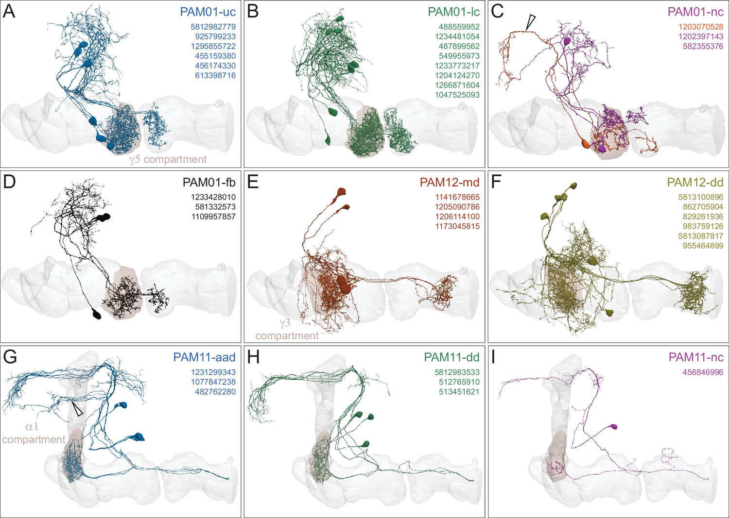
Anatomy of PAM01, PAM12, and PAM11 DAN subtypes.
Morphologies of DAN subtypes discussed in Figure 28. Innervated MB lobes are shown in gray and the relevant compartment in brown. (A) Six PAM01-uc DANs (blue) project across the upper commissure (uc). (B) Eight PAM01-lc DANs (green) project across the lower commissure (lc). The dendritic field of PAM01-lc also extends slightly more anterior and ventral compared to PAM01-uc DANs (A). (C) Three non-canonical (nc) PAM01-nc DANs (magenta and orange) shown together. A single PAM01-nc DAN (orange, crossing the lc) has an additional dendritic branch in the SLP (indicated by hollow arrowhead) and two other PAM01-nc DANs (1202397143, 582355376, crossing the uc) have axons confined to the dorsal or lateral portion of the γ5 compartment. Note that PAM01-nc (582355376) has been classified as PAM08 in the hemibrain v1.1 release. (D) Three PAM01-fb DANs receive direct feedback (fb) from MBON01 (γ5β'2a) and their presynaptic fields are confined to the ventral portion of the γ5 compartment, in contrast to other PAM01 DANs. They also project through the lower commissure. Subtypes match those in Otto et al., 2020. (E–F) PAM12 DANs divide into (E) four medial dendrite (md) PAM12-md DANs (maroon) and (F) six dorsal dendrite (dd) PAM01-dd DANs (ochre) (also see Figure 32). (G–I) The three morphological groups of PAM11 DANs. These DANs are also shown in Figure 29—video 1. (G) Three PAM11-aad DANs (blue) have an additional anterior dendrite (aad) anterior to the α lobe (arrowhead). (H) Three dorsal dendrite (dd) PAM11-dd DANs (green). (I) One non-canonical (nc) PAM11-nc DAN (magenta), which unlike the other PAM11 DANs, has an axonal field confined to the middle of the α1 compartment.
Figure 29 with 4 supplements
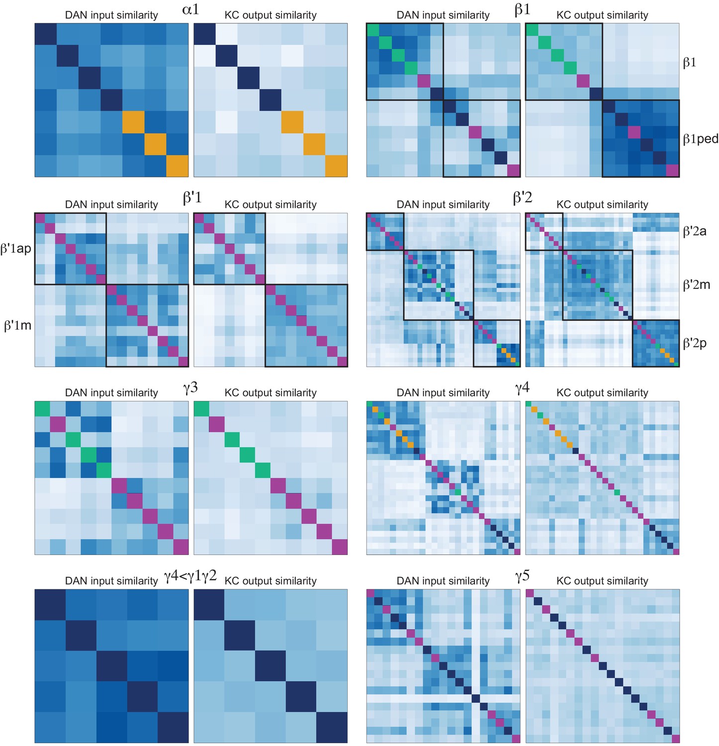
Relationship between DAN dendritic inputs and DAN axonal outputs to KCs.
These plots explore whether DANs of the same cell type that have distinct inputs also connect to distinct populations of KCs within a compartment. Analysis of eight compartments is shown. Within each example, the left heatmap represents the similarity of input to DANs (identical to the corresponding block in Figure 27). The right heatmap represents the cosine similarity of the output synapses made by DANs onto KCs. The clustering observed in the right panels most likely results from individual PAM neurons only arborizing in a portion of their compartment (see neuronal morphologies Figure 28—figure supplement 1 and Figure 30). Such clustering may permit specific reinforcement signals to be conveyed to subsets of KCs within a compartment. See detailed discussion of DAN-KC connectivity in Figure 30 and Figure 30—figure supplements 1 and 2. The potential computational significance of this phenomenon is explored in the Discussion (see Figure 38). Additional anatomical information about DAN cell types PAM11 (a1), PAM09 (b1-ped), PAM12 (g3) and PAM07 (g4<g1g2) is presented in Figure 29—video 1, Figure 29—video 2, Figure 29—video 3, Figure 29—video 4, respectively.
Figure 29—video 1
PAM11 (α1) dopaminergic neurons.
Figure 29—video 2
PAM09 (β1-ped) dopaminergic neurons.
Figure 29—video 3
PAM12 (γ3) dopaminergic neurons.
Figure 29—video 4
PAM07 (γ4<γ1γ2) dopaminergic neurons.
Figure 30 with 3 supplements
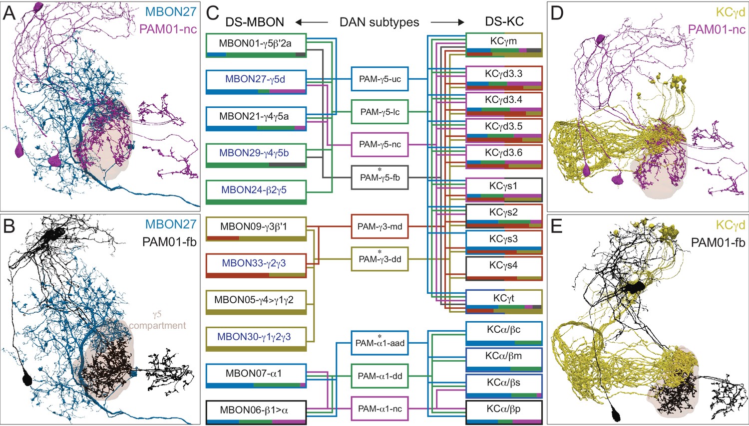
Different subtypes of the PAM01, PAM12, and PAM11 DANs synapse onto specific subpopulations of KCs and MBONs within their compartment.
KCs are subtyped as shown in Figure 4—figure supplements 1, 2 and 4. The axons from certain subtypes of DAN occupy different regions of, and together tile, a MB compartment. This permits for specific connectivity to KCs and MBONs within the compartment. A zonal subcompartment arrangement is a feature of many MB compartments and is illustrated here by the distinct morphologies of two subtypes of the γ5 compartment DANs (A, B, D, E). Implications for connectivity of this type of restricted DAN arborization are summarized for the γ5, γ3, and α1 compartments in panel C. Figure 30—figure supplements 2 and 3 show connectivity matrices for additional compartments in the right hemisphere. (A) The axons from PAM01-nc (magenta) overlap with dendrites of MBON27 (γ5d; dark blue). Note that the axons of the two PAM01-nc DANs (magenta) are confined to the dorsal and lateral region of the γ5 compartment (see also Figure 28—figure supplement 1C). (B) PAM01-fb (black) axons do not overlap with the dendrites of MBON27 (dark blue). (C) Schematic of the innervation of subtypes of γ5, γ3, and α1 DANs within the compartment showing their connection to MBONs (left) and KCs (right). Boxes for DAN subtypes and connectivity edges are colored according to subtype identity. Boxes around MBON types are colored by their strongest DAN subtype input. The boxes around KC names are colored to reflect their strongest DAN subtype input in each compartment (the two halves for KCγ types reflect their projections through the γ3 and γ5 compartments). Horizontal bars along the lower edge of the MBON and KC boxes are histograms, with bar colors corresponding to DAN subtypes, representing the proportion of each DAN subtype providing input to the respective MBON or KC subtype. For the KCγ types, the upper bar represents inputs in γ5 and the lower bar in γ3. Typical MBON names in black and atypical MBONs are in blue. Asterisks denote DAN subtypes receiving MBON feedback (compare with Figures 26–28). Only cases where a DAN provides at least 0.1% of the MBON’s synaptic input or at least 1% of a KC type’s input from DANs are shown. KC cell types are biased in their representation of different sensory modalities (Figure 15—figure supplement 2). Note that the synapses onto the feedforward MBON06 (β1>α) are likely axo-axonal. (D) The axons from PAM01-nc (magenta) also overlap with the axonal processes of KCγd (yellow). (E) Axons from PAM01-fb (black) do not overlap with the axonal processes of KCγd (yellow).
Figure 30—figure supplement 1
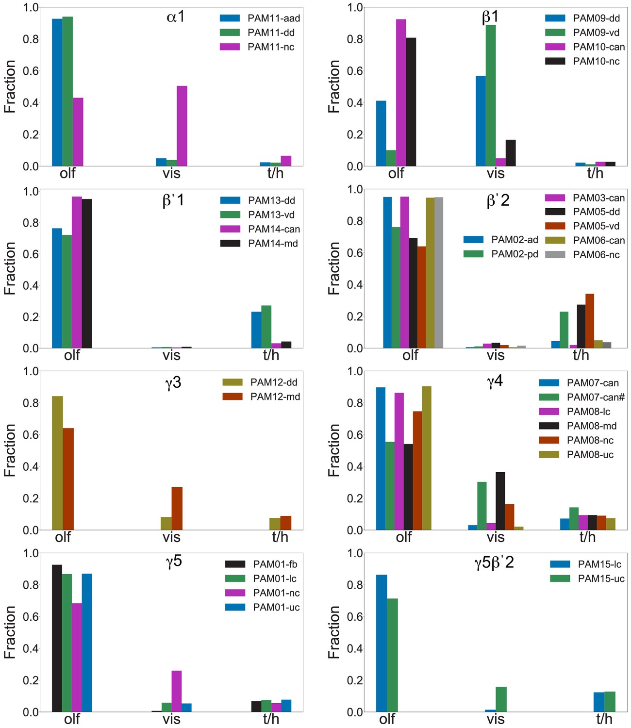
DAN subtypes within a compartment can be biased toward KC types representing different sensory modalities.
These plots reveal that in many cases, selective innervation of KC subclasses by particular DAN subtypes within a compartment is organized according to the sensory modality represented by those KCs. Sensory modalities of KCs are assigned according to their PN inputs (derived from the same data as Figure 15—figure supplement 2A). In the indicated compartments, the DANs of a given type are divided into subtypes following criteria from Figure 28. For the PAM07-can (γ4<γ1γ2) subtype, one outlier, indicated by the # sign, which was not apparent with clustering either by morphology or input connectivity, was identified by spectral clustering of DAN-KC connectivity (Figure 29). The y-axis values indicate the fraction of each of the indicated DAN cluster’s output it provides to KCs representing three different sensory modalities. The contributions of each KC to this value are weighted by the number of input synapses they receive from DANs of the given type. Olf - olfactory, vis - visual, and t/h - thermo/hygrosensory.
Figure 30—figure supplement 2
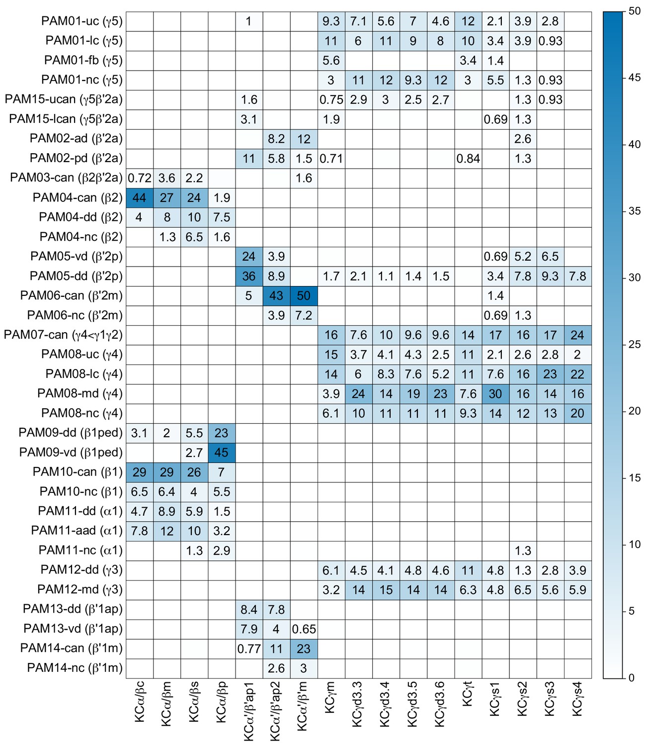
Within a compartment PAM DAN subtypes synapse onto specific KC subtypes as defined by the clustering shown in Figure 4—figure supplements 1, 2 and 4.
DAN to KC connectivity matrix underlying Figure 30. DAN subtypes, defined by morphological and upstream connectivity clustering (see Figure 28), synapse onto specific types of KCs within a compartment. Each cell of the matrix shows the percentage of inputs provided by a particular DAN subtype, normalized by all DAN inputs to that KC type. DAN subtypes that have axons confined to portions of the same compartment often differ in their KC connectivity. Only connections constituting greater than 0.5% of the KC’s total DAN input in the compartment are shown.
Figure 30—figure supplement 3
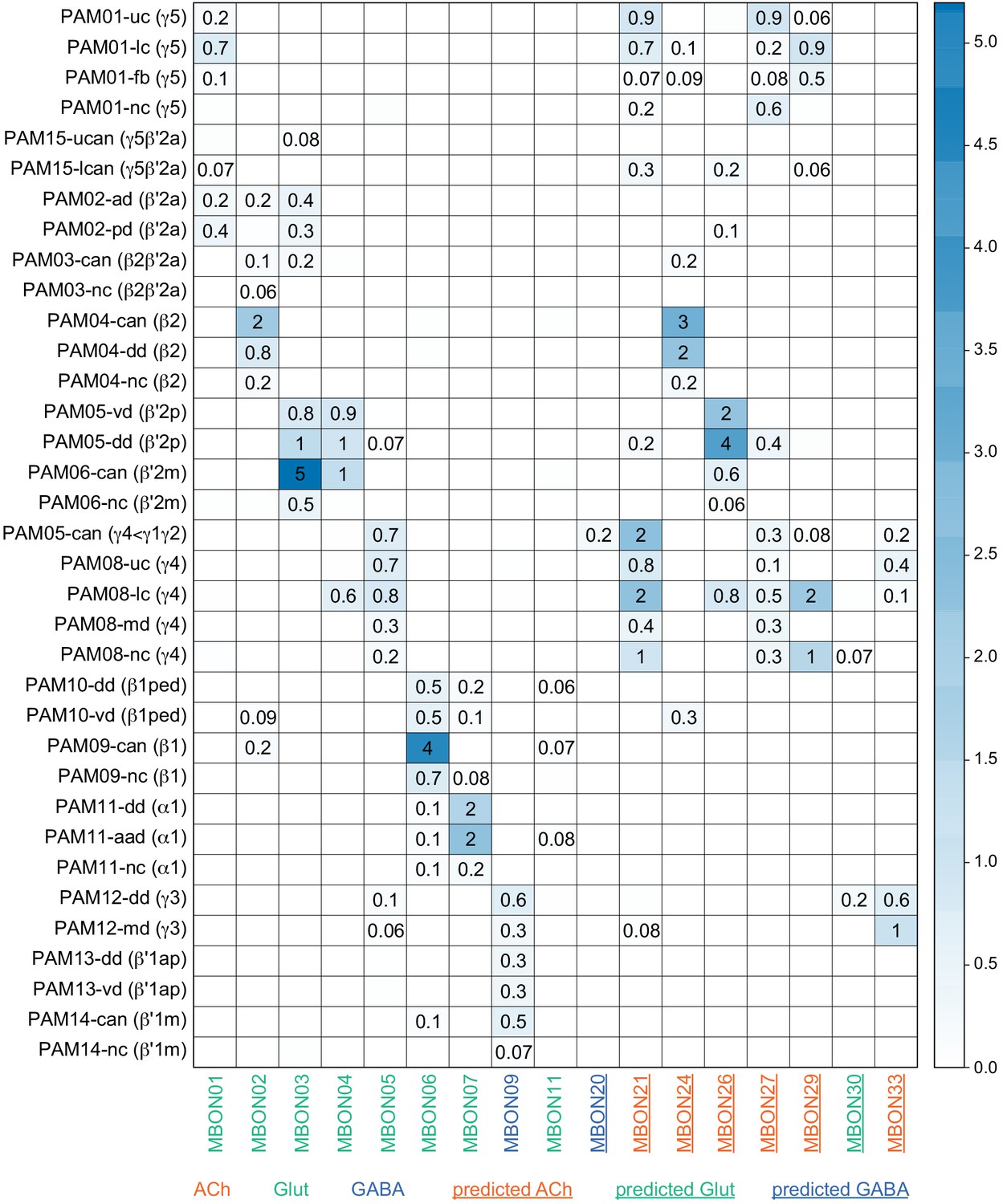
PAM DAN subtypes synapse selectively onto particular MBONs within a compartment.
DAN to MBON connectivity matrix underlying Figure 30. DAN subtypes as defined by morphological and upstream connectivity clustering (from Figure 28) connect to specific MBONs within the respective compartment. Each cell of the matrix shows the percentage of input provided by the indicated DAN subtype, normalized by the MBON’s synaptic input. DAN subtypes that have axons confined to a specific portion of the same compartment often differ in their connectivity to MBONs. Only connections constituting greater than 0.1% of the synaptic input to each MBON are shown.
Figure 31
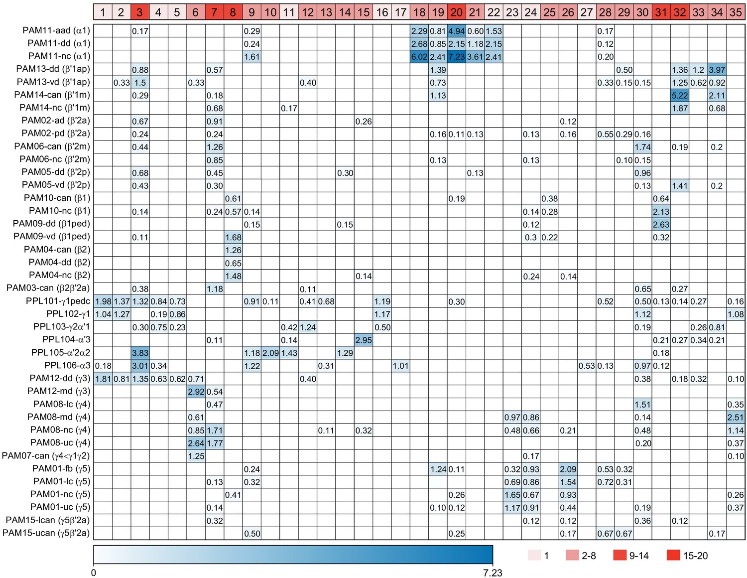
Shared input neurons reveal expected and unexpected across-compartment groupings of DAN subtypes.
Matrix representing the connectivity to DAN subtypes provided by the top 50 strongest input neurons to each DAN subtype in the right hemisphere (n = 901 neurons, excluding MBONs and MB intrinsic neurons). These inputs are either unique individual neurons (clusters of one) or clusters of multiple neurons grouped according to their morphology. A selection of 35 input clusters are shown, numbered in boxes whose shading reflects the number of neurons that contribute to that cluster (input clusters are listed in Supplementary file 2). Each cell represents the proportion of the total inputs to the dendrites of the DANs of the respective subtype (y-axis) provided by the input neuron cluster (x-axis). Selected input clusters and innervation patterns are further explored in Figures 32–37. Some DAN subtypes receive inputs from neurons projecting from heavily studied neuropils like the SEZ, the FB, and the LH; for example, clusters 10, 18, 19, 20, 21, 22, 23, 24, 25, 26, 27, 28, 31 (Figures 33–35). Many clusters selectively connect to groups of DAN subtypes of the PAM or PPL1 type specifically; for example, clusters 7, 8, 11, 12, 13, 14, 15, 29, 32 (Figure 36) and clusters 22, 23, 24, 26, 27 (Figure 35). Some input neuron clusters connect DAN subtypes with opposite/mixed valence; for example, clusters 3, 9, 30, 33, 35 (Figure 37) and cluster 28 (Figure 35; also see Otto et al., 2020). Input neuron clusters can also stand out by the DAN subtypes that they avoid; for example, clusters 3 and 30 (Figure 37). The matrix was thresholded to show inputs over 0.1% of total input to DAN dendrites and the threshold for strong connectivity was defined as 0.5%. The neuropil of the SEZ is not included in the hemibrain database. Therefore, more complete anatomy of DAN input neurons from this region were retrieved from FAFB (Zheng et al., 2018 ; see Figure 35).
Figure 32 with 1 supplement
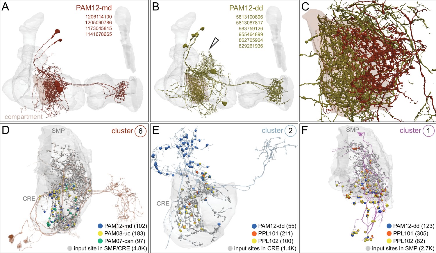
Morphologically distinct subtypes of PAM12-DANs share inputs with either PPL1 or PAM DANs.
(A) The four PAM12-md DANs (maroon) innervate the γ3 compartment (brown) of the MB (gray ). (B) The PAM12-dd subtype (green) has additional dorsal dendritic branches (hollow arrowhead) not found in PAM12-md. A seventh PAM12-dd that lacked its ipsilateral axon was excluded from the analysis. (C) The axonal fields of PAM12-md and PAM12-dd DAN subtypes tile the γ3 compartment (brown), suggesting they modulate different downstream neuronal connections (see Figure 30 and Figure 39 for further analyses and discussion). (D–F) Strong inputs (see Figure 31) to PAM12-md also specifically synapse onto positive-valence PAM DANs, whereas PAM12-dd shares inputs with negative-valence PPL1 DANs; synapse numbers are given in parentheses. Circled number in the upper right of each panel refers to the input cluster number in Figure 31. (D) Cluster 6 collectively provides the strongest dendritic input to PAM12-md DANs (blue dots) and is also the strongest input to two DAN subtypes innervating γ4, PAM08-uc DANs (yellow dots) and canonical (can) PAM07-can (green dots). In addition, cluster 6 connects to other PAM08-DANs, but excludes the lower commissure (lc) subtype. (E) A single, morphologically distinct neuron (cluster 2) connects to the positive valence PAM12-dd (blue dots) and the negative-valence PPL101 (γ1pedc) (orange dots) and PPL102 (γ1; yellow dots). (F) This single (cluster 1) neuron provides the strongest dendritic input to positive-valence PAM12-dd (blue dots) and the negative-valence PPL101 (γ1pedc; orange dots) and also synapses onto PPL102 (γ1; yellow dots) DANs. Connections contributing less than 1% of a neuron’s total dendritic input have been excluded. See Figure 32—figure supplement 1 for further morphological details.
Figure 32—figure supplement 1
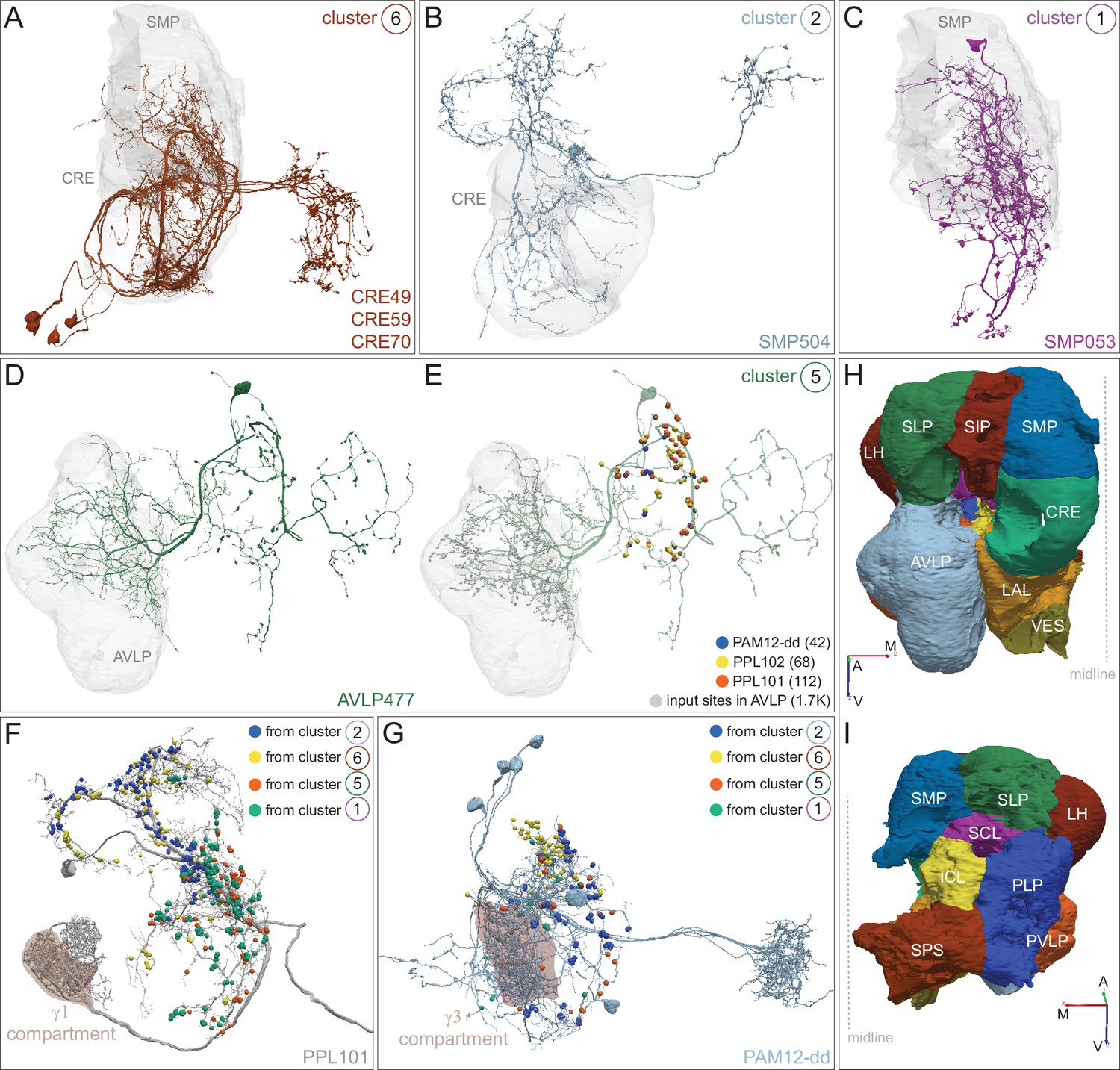
Strong inputs to PAM12-dd and PPL101 localize to different dendritic arbors.
More detailed representations of connectivity between input clusters 6, 2, 1, and 5 (Figure 31) and PPL101 and PAM12-dd DANs. Neuropils in which DAN input neurons receive most of their inputs are shown in gray. (A–C) Neurons in cluster 6 (cell types CRE049, CRE059, CRE070), cluster 2 (cell type SMP504) and cluster 1 (cell type SMP053), shown in Figure 32D–F are shown here without their output synapses marked to allow better visibility of their morphologies. (D and E) Cluster 5 (cell type AVLP477) shown without synapses (D) and with synapses marked (E) also synapses onto PAM12-dd (blue dots), PPL101 (γ1pedc; orange dots) and PPL102 (γ1; yellow dots) DANs; synapse numbers are given in parentheses. (F) Detail of inputs to PPL101, whose outputs are in the γ1 compartment (brown) and the core of the pedunculus. Inputs from valence-specific clusters 2, 6, 5, and 1 (synaptic input color-coded as indicated) localize to specific branches of PPL101. (G) Detail of inputs to PAM12-dd, whose outputs are in the γ3 compartment (brown) and which receives input from clusters 2, 6, 5, and 1 (synapses color-coded as indicated). While clusters 5 and 2 inputs are evenly distributed, cluster 6 and 1 localize to the dorsal portion of the PAM12-dd’s dendrites. (H and I) Two views of the input neuropils discussed in Figures 32–36; see Figure 2—figure supplement 1 for a key to abbreviations. Connections contributing less than 0.5% of a neuron’s total dendritic input have been excluded.
Figure 33 with 1 supplement
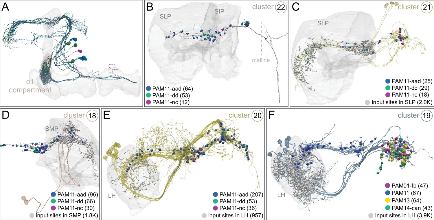
Examples of local neurons, SEZONs, and LHONs that target PAM11 DANs.
(A) All PAM11 DAN subtypes are shown, color-coded as in Figure 28 and Figure 28—figure supplement 1; the MB lobes are shown in gray and the α1 compartment is shaded brown. (B–F) Examples of neurons from clusters in Figure 30 that provide strong input to PAM11 DANs or to PAM11 and other positive-valence PAM DANs are shown; cluster identity is indicated by the circled number in the upper right of each panel. Neuropils where DAN input clusters receive their inputs are shown in gray (except for SEZONs whose dendrites are not in the hemibrain volume) and position of output synapses to PAM11 subtypes are shown color-coded; synapse numbers are given in parentheses. Figure 33—figure supplement 1 shows more information about the neurons constituting these clusters. (B) The single neuron in cluster 22, a SEZON, makes synapses to all three subtypes of PAM11 DANs; PAM11 DANs are the only DAN targets of cluster 22. The same applies to its contralateral partner (see Figure 35—figure supplement 1A). (C) The local interneurons that make up cluster 21 receive inputs in the SLP and connect to all three PAM11 subtypes, but not to other DANs. (D) The local interneurons that make up cluster 18 (299626157, 361700223) receive inputs in the SMP and connect to PAM11 DANs, but not to other DANs. (E) LHON cluster 20 connects to all three PAM11 subtypes and weakly to PAM01 and other positive-valence PAM DANs. (F) The LHONs cluster 19 connect to all three PAM11 subtypes and also to PAM13 (β′1ap), PAM14 (β′1m) and PAM01-fb (γ5) DANs (compare to Frechter et al., 2019, Dolan et al., 2019 , and Otto et al., 2020). The connections to the PAM11 and the other PAM DANs are located on different primary branches of the cluster 19 neurons. Connections contributing less than 0.5% of a neuron’s total dendritic input have been excluded.
Figure 33—figure supplement 1
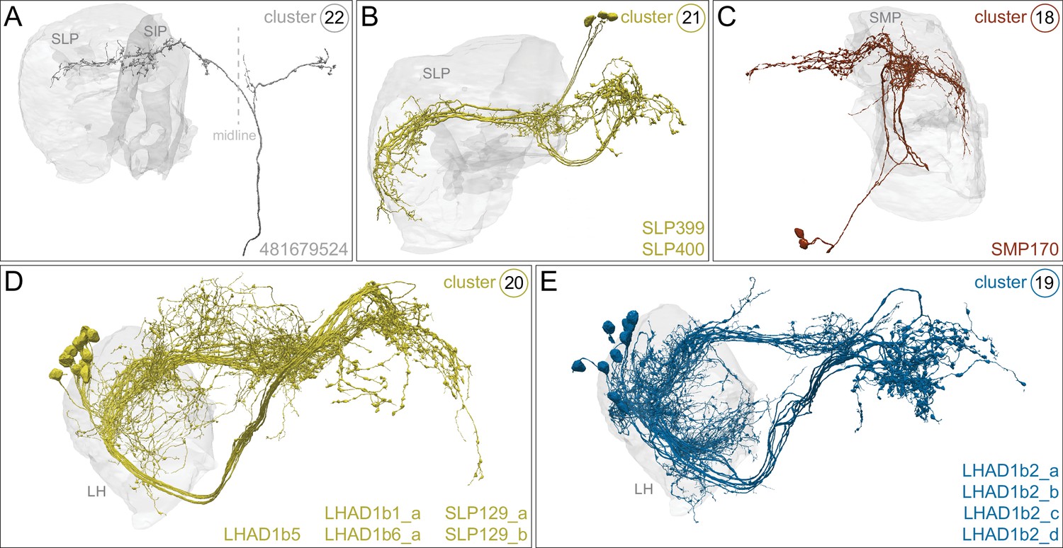
More information on the cell types shown in Figure 33.
Figure 34
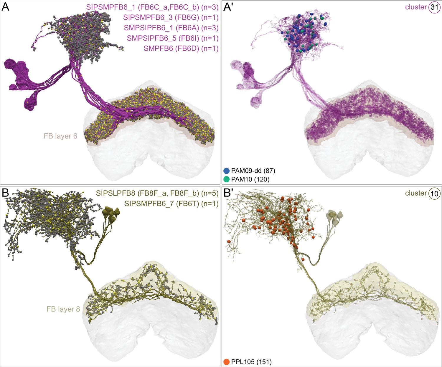
Distinct FB neurons provide input to β lobe PAM or PPL105 DANs.
Two morphological clusters (31 and 10, Figure 31) of neurons from FB are among the strongest DAN inputs. These FB neurons have arbors of mixed polarity both in the SMP and in the FB, as can be seen in panels A and B where their presynaptic and postsynaptic sites are shown in yellow and gray , respectively. (A-A′) Cluster 31 neurons are shown in magenta and consists of nine FB layer 6 neurons of five cell types. These neurons synapse onto the dendrites of three potentially positive-valence PAM DAN subtypes: PAM09-dd (β1ped; blue dots), and two β1 DAN subtypes, PAM10-can and PAM10-nc(dd) (combined in figure; green dots); synapse numbers are given in parentheses. Remarkably, seven of the nine neurons of cluster 31 are connected, via an interneuron, to MBON19 (α2p3p; see Figure 20—figure supplement 1C and Figure 20—video 4). (B-B′) Cluster 10 neurons are shown in yellow and consist of five layer 8 (cell type: SIPSLPFB8) and one layer 6 FB neurons and make synapses in the SMP onto PPL105 (α′2α2; orange dots; synapse number is given in parentheses); the negative-valence PPL105 is the only DAN they innervate. Connections contributing less than 0.5% of a neuron’s total dendritic input have been excluded.
Figure 35 with 1 supplement

Output neurons from different areas of the SEZ tile the SMP where they synapse onto select DAN subtypes.
(A) Axons from multiple SEZON cell types in clusters 22, 23, 24, 25, 26, 27, and 28 (see Figure 31) that provide strong inputs to DAN subtypes are shown together. (A′) The same SEZON axons shown with synapses connecting to PAM DANs (blue, from five clusters) and to PPL1 DANs (orange, from two clusters); synapse numbers are given in parentheses. (B) The five neurons of SEZON cluster 28 (light blue; these neurons correspond to the SEZON01 cluster 5.4.1 of Otto et al., 2020) branch in the SMP and synapse onto the PPL101 (orange), PAM01-lc (black), PAM01-fb (dark yellow), PAM02-pd (green), and PAM15-uc (yellow) subtypes; synapse numbers are given in parentheses. (C) The single neuron in SEZON cluster 27 (green) branches in the SMP and SIP and synapses only onto PPL106; synapse number is given in parentheses. (D) The single neuron in SEZON cluster 23 (gray) branches in the SMP and connects to positive-valence DANs: PAM01-lc (yellow), PAM01-uc (green), PAM01-nc (blue), and PAM08-md (magenta); synapse numbers are given in parentheses. (E) The axons of SEZON neurons can be matched to those in the FAFB EM volume (Zheng et al., 2018) to permit the retrieval of their dendritic field, which resides in tissue that is missing from the hemibrain dataset; skeleton ID numbers from FAFB are shown. FAFB matches to hemibrain SEZONs are shown and colored to match their hemibrain counterparts (colors correspond to those used in panels B-D); the SEZON 551939 was traced in the left hemisphere in FAFB and a mirror image is shown here to facilitate comparison. Their dendritic fields differ, suggesting these SEZON clusters are likely to convey distinct information. Connections contributing less than 0.5% of a neuron’s total dendritic input have been excluded.
Figure 35—figure supplement 1
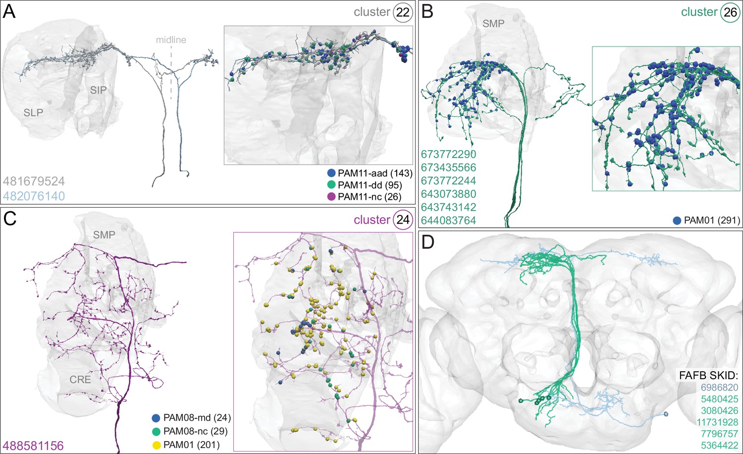
Most strongly connected SEZON clusters exclusively synapse onto positive-valence PAM DANs.
(A–C) Further examples of clusters consisting of SEZONs that connect to specific DAN subtypes. In each panel the neuronal morphology is shown on the left with the brain regions where they contact DANs shown in gray , and on the right a higher magnification view of their output synapses onto specific DAN types are shown, color-coded , with synapse numbers given in parentheses. The threshold for connectivity is 0.5% of the DANs total inputs (Figure 31). (A) The neurons of SEZON cluster 22 (481679524) and its contralateral partner (482076140) branch in the SMP and SLP and synapse onto all 3 PAM11 subtypes (compare to Figure 33). (B) The six neurons in SEZON cluster 26 branch in the SMP and connect to positive-valence γ5 DAN subtypes (blue) and weakly to PAM15 (γ5β′2a) and PAM02 (β′2a) subtypes. (C) The single neuron in SEZON cluster 24 branches in the SMP and connects specifically to PAM08-md (γ4; blue) and PAM08-nc subtypes (green), all PAM01 (γ5) subtypes (yellow). (D) The axons of SEZONs in (A and B) can be matched to those in the FAFB EM volume (Zheng et al., 2018). This registration permits the retrieval of their dendritic fields, which reside in tissue that is missing from the hemibrain dataset. FAFB matches to hemibrain SEZONs are shown and are colored to match their hemibrain counterparts in panels (A) and (B). The dendritic fields differ, suggesting these SEZONs convey distinct information. Connections contributing less than 0.5% of a neuron’s total dendritic input have been excluded.
Figure 36 with 2 supplements
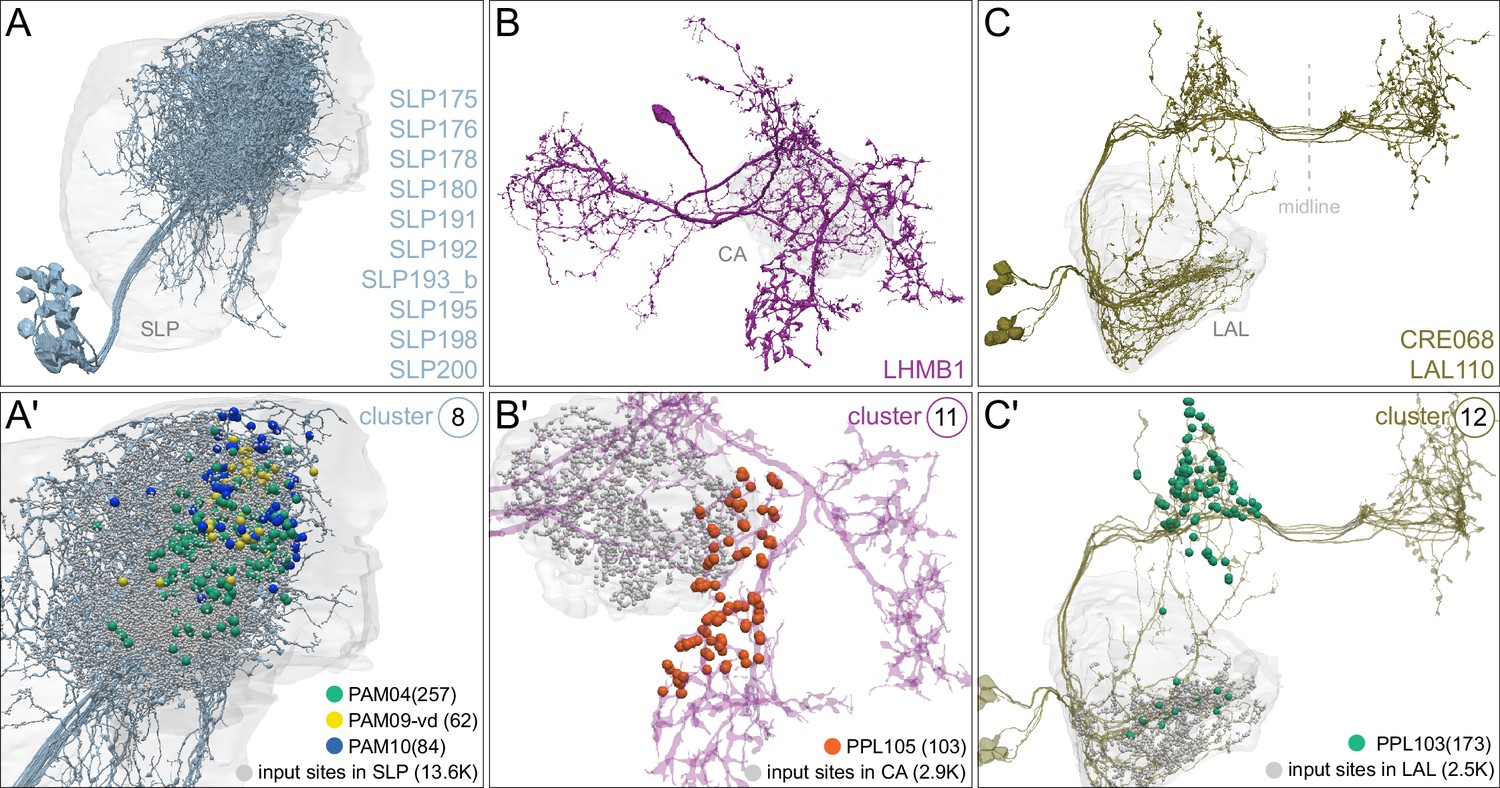
A number of input neurons specifically target DAN groups of the PAM or PPL1 clusters.
Neurons providing strong input to PAM or PPL1 DANs are shown. Neuropil areas of inputs to these neurons are shown in gray in (A–C) and synapses to DANs are shown color-coded in (A′-C′); synapse numbers are given in parentheses. The threshold for connectivity is 0.5% of the DANs total inputs (Figure 31). (A-A′) Cluster 8 is comprised of 20 neurons of 10 similar cell types which provide input to subtypes of β-lobe PAM DANs in the SLP: PAM10 (β1; blue); PAM09-vd (β1ped; yellow) and all PAM04 subtypes (β2; green). (B-B′) The single neuron in cluster 11 receives inputs in the CA and connects to PPL105 (α′2α2; orange). (C-C′) The seven neurons in cluster 12 (LAL110, CRE068) receive inputs in the LAL and provide the strongest input to PPL103 (γ2α′1; green). Connections contributing less than 0.5% of a neuron’s total dendritic input have been excluded.
Figure 36—figure supplement 1

Inputs specific to PAM DANs.
Neurons providing strong input to DANs of the PAM cluster are shown. Neuropil areas indicated (gray) and synapses to DANs are color-coded ; synapse numbers are given in parentheses. (A-A′) The seven neurons of cluster 29 fall into seven cell types, receive inputs in the SMP and connect to PAM15-uc (γ5β′2a; orange) and the PAM13-dd (β′1ap; green). (B-B′) The 12 neurons of cluster 7 fall into four cell types, receive inputs in the SMP and SIP and connect strongly to PAM DANs that are restricted to the β′ (blue synapses) and the γ lobes (green synapses): PAM13 (β′1ap), PAM14 (β′1m), PAM02 (β′2a), PAM06 (β′2m), PAM05 (β′2p), PAM03 (β2β′2a) and PAM12-md (γ3), PAM08 (γ4), PAM01 (γ5), PAM(γ5β′2a). (C-C′) Cluster 32 has nine neurons of four cell types that receive some inputs in the CRE. Cluster 32 provides strong input to PAM14 (β′1) subtypes (orange synapses) and is also upstream of the PAM05-vd (β′2p) subtype (blue synapses) and all PAM13 (β′1ap) subtypes (green synapse). The threshold for connectivity is 0.5% of the DANs total inputs (Figure 31).
Figure 36—figure supplement 2
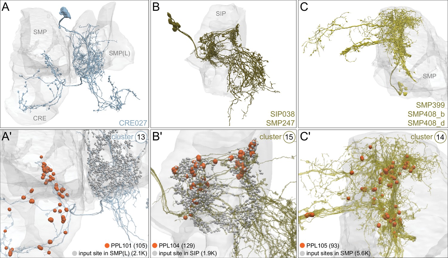
Inputs specific to PPL1 DANs.
Neuropil areas indicated (gray) and synapses to DANs are color-coded ; synapse numbers are given in parentheses. (A-A′) The two neurons (light blue) of cluster 13 receive inputs in the contralateral SMPs and connect to the negative-valence PPL101(γ1pedc; red) DANs. (B-B′) Cluster 15 has five neurons receiving inputs in the SIP and provides strong input to PPL104 (α′3). (C-C′) The seven neurons of cluster 14 receive inputs in the SMP and are strongly connected to the PPL105 (α′2α2). The threshold for connectivity is 0.5% of the DAN’s total inputs (Figure 31).
Figure 37 with 1 supplement
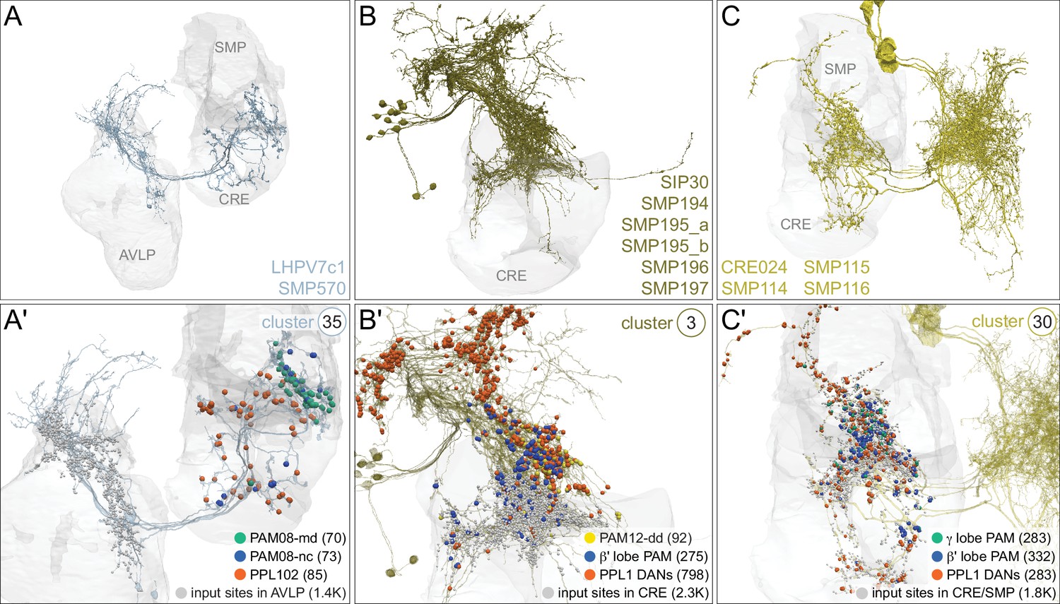
Neurons that provide strong input to both PAM and PPL1 DANs.
Neuropil areas indicated in gray and synapses to DANs are color-coded ; synapse numbers are given in parentheses. (A-A′) The four neurons of cluster 35 receive inputs in the AVLP and provide strong input to the PAM08-md (γ4; green) and PAM08-nc (blue synapses) subtypes as well as the PPL102 (γ1) DAN (orange synapses). (B-B′) The 13 neurons of cluster 3 receive some inputs in the CRE; they constitute the strongest input to PPL105 (α′2α2) and PPL106 (α3) and also connect to PPL101 (γ1pedc), PPL102 (γ1), and PPL103 (γ2α′1) (all PPL1 DAN synapses combined, red), all of the β′ lobe PAM DAN subtypes (blue synapses) and the PAM12-dd (γ3) subtype (yellow synapses). (C-C′) Cluster 30 has four neurons that receive inputs in the SMP and CRE and are upstream of negative-valence PPL1 neurons (PPL101, PPL102, PPL105, and PPL106; orange synapses) and PAM DANs innervating the β’ (blue synapses) and γ (green synapses) lobe (PAM08, PAM01, PAM03, PAM05, PAM06). While both cluster 3 and 30 connect to both PPL1 and PAM DANs, cluster 30 connects to γ lobe PAM DANs, in contrast to cluster 3 favoring β′ lobe PAM DANs.
Figure 37—figure supplement 1
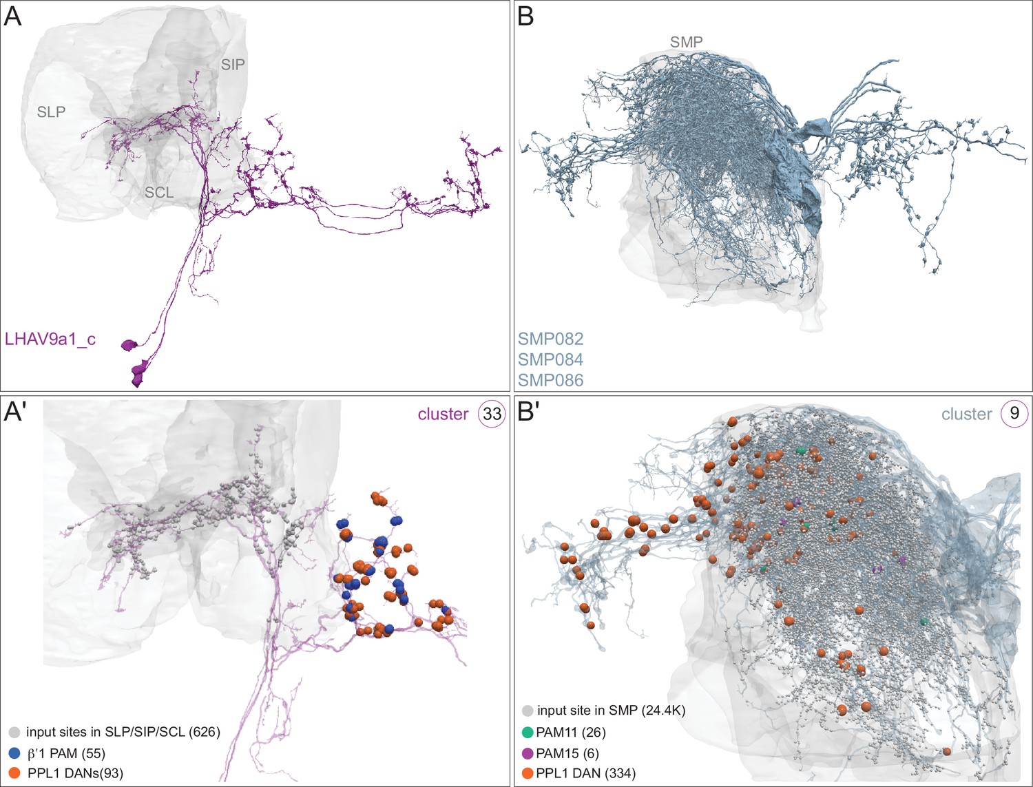
Additional examples of neurons providing common input to both PAM and PPL1 DANs.
Neuropil areas where neurons of clusters 33 and cluster 9 receive input are shown in gray and their synapses onto DANs are color-coded ; synapse numbers are given in parentheses. (A-A′) The three neurons of cluster 33 receive inputs in the SIP, SLP, and SCL and connect to both PAM13 (β′1ap) subtypes (blue synapses) and to a collection of PPL1 DANs (PPL101, PPL102, PPL103 and PPL104; red synapses). (B-B′) Cluster 9 has six neurons that receive inputs in the SMP and connect to the negative-valence PPL1 DANs (PPL101, PPL102, PPL105 and PPL106; orange synapses). Cluster 9 is also upstream, but more weakly, of positive-valence PAM DANs including all PAM11 subtypes (green synapses), the PAM15 subtypes (magenta synapses) and more weakly to PAM01-lc and PAM01-fb subtypes.
Figure 38
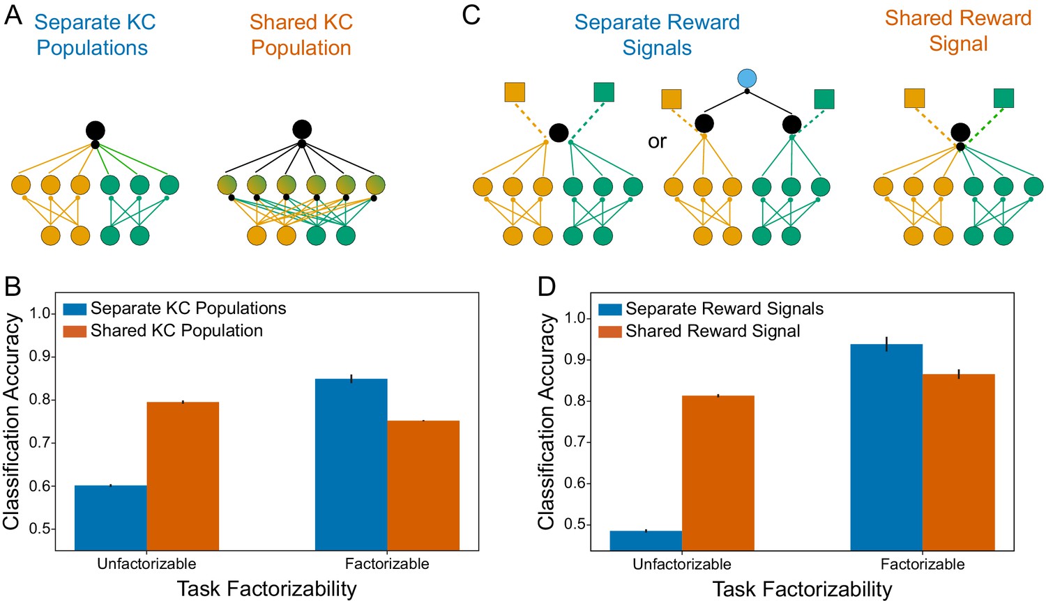
Effects of segregated or mixed-modality signals.
(A) Schematic of two possible architectures for an MB-like circuit, in which KCs are either specialized for one sensory modality (left) or receive mixed input (right). Bottom layer circles represent PN inputs, middle layer circles represent KCs, and black output circles represent MBONs. Green and yellow shades indicate different sensory modalities. (B) Task performance in a stimulus discrimination model for the architectures shown in A. Stimuli consist of random binary patterns in two sensory modalities. In the ‘factorizable’ task, the stimulus from each modality has an assigned valence (positive or negative) and the overall valence is positive only if both constituent valences are positive. In the ‘unfactorizable’ task, each stimulus is randomly assigned its own unique valence, irrespective of its constituent modalities. A linear readout, modeling an MBON, is fit to discriminate the valences of the stimuli based on the activations of the KC population. The linear fit procedure corresponds to the experienced-based plasticity of KC-MBON synapses. Task performance is defined as the binary classification accuracy—that is, the frequency with which the thresholded response of the MBON corresponds correctly to the valence of the input—of this MBON readout. 25 stimuli are presented in the unfactorizable task and 200 in the factorizable task, to make overall task difficulty comparable. Error bars represent standard error over 20 simulations. (C) Schematic of possible architectures for DAN-dependent plasticity in an MB-like circuit. In the leftmost model, DANs (colored squares) modulate KC-MBON synapses for KCs of a particular sensory modality. The second-to-left model depicts two MBONs, each integrating input from KCs of a particular sensory modality, and each with its own corresponding DAN, that additively converge onto a common output (blue). These two models are functionally equivalent, and hence are grouped together under ‘separate reward signals.’ In the rightmost model, there is a single MBON, and DANs modulate all the KC-MBON synapses (right). (D) Task performance in a stimulus discrimination model (same as B) for the architectures shown in C. For each task the optimal KC structure from B is used (‘separate’ for the factorizable task, ‘shared’ for the unfactorizable task).
Figure 39
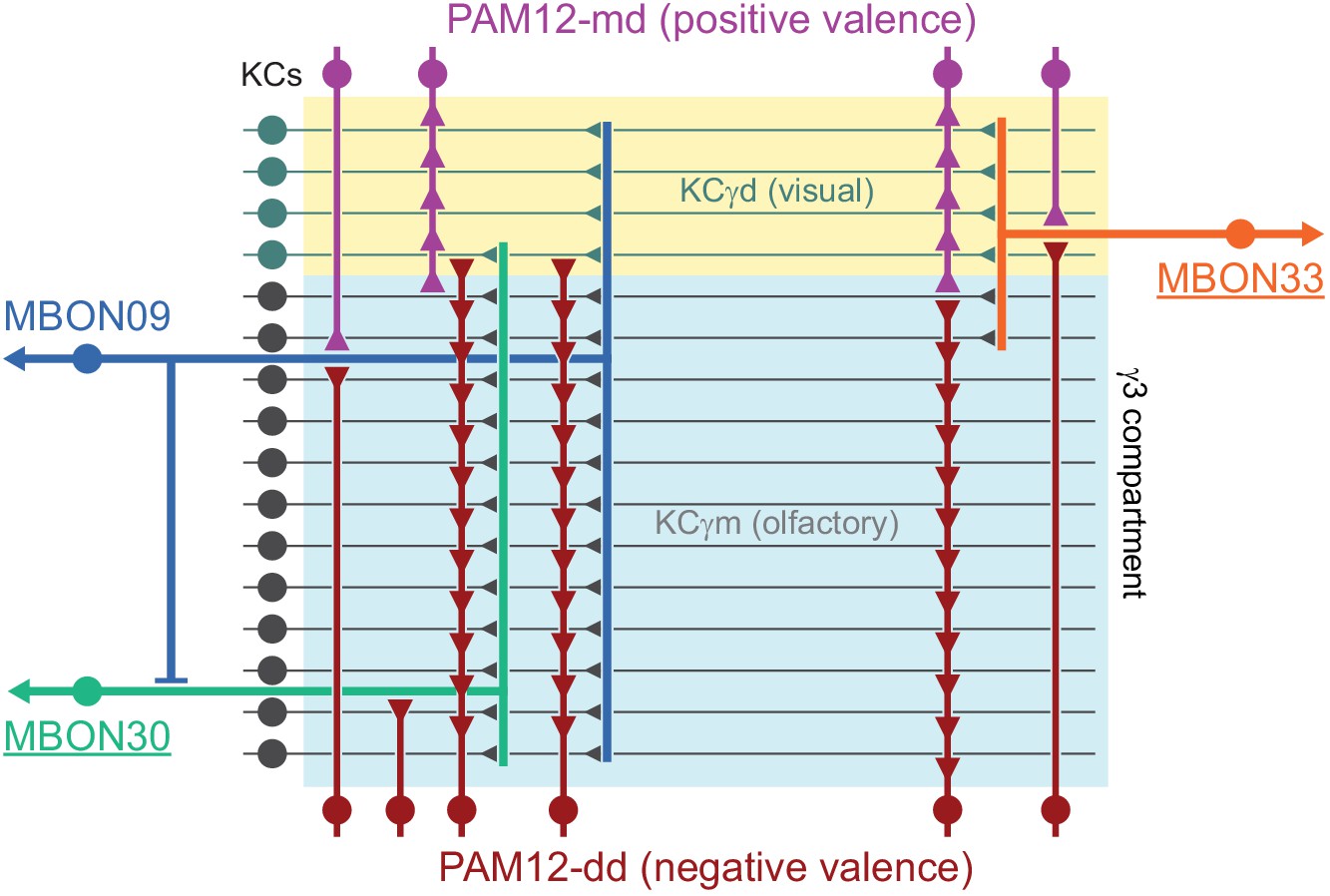
Schematic of subcompartment DAN and MBON innervation within γ3.
The two PAM12 (γ3) DAN subtypes likely represent opposite valence based on their shared input with either aversively reinforcing PPL1-DANs or appetitively reinforcing PAM08 (γ4) DANs. Whereas PAM12-md DANs selectively innervate the visual γd KCs, the PAM12-dd DANs innervate both γd and γm (olfactory) KCs. The dendrite of atypical MBON30 is restricted to the olfactory γm (olfactory) KCs and its DAN input is exclusively from the PAM12-dd subtype. In contrast, the dendrite of atypical MBON33 preferentially collects γd KC input and receives input from both PAM12-md and PAM12-dd DANs. The GABAergic MBON09 (γ3β′1) pools γm and γd KC input, receives DAN input from PAM12-md and selectively synapses onto MBON30.
Figure 40

MBON network representation of aversive memory.
Shock responsive DANs innervating γ1, γ2 and γ3 depress odor-specific KC synapses onto the respective MBONs. Depression of MBON11 (γ1pedc>α/β) and MBON09 (γ3β′1) releases their feedforward inhibition onto the avoidance-directing γ5 and β′2 MBONs. In addition, MBON11 release increases the inhibitory effect of the MBON06 (β1>α) onto the approach-directing α1 and α3 compartments. Repetitive aversive training trials, and a release from inhibition also allows the DANs in α2 and α3 to depress odor-specific KC synapses onto the respective approach- directing MBONs. These changes together leave the network in a configuration to direct strong odor-specific avoidance behavior.
Figure 41
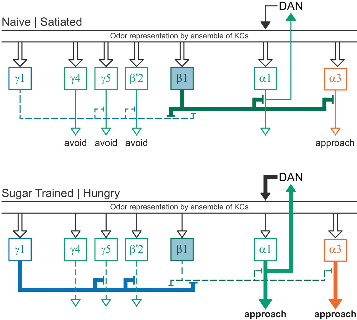
MBON network representation of appetitive memory.
Sugar-responsive DANs innervating γ4, γ5, β′2, and β1 depress odor-specific KC synapses onto the respective MBONs. Depression of the odor-specific response of MBON06 (β1>α) reduces odor-specific feedforward inhibition onto the MBON07 (α1) and MBON14 (α3). This frees α3 to direct odor-driven approach behavior and increases activity in a recurrent α1 MBON07-PAM11aad DAN loop to consolidate long-term appetitive memory. MBON11 (γ1pedc>α/β) is sensitive to satiety state and is more responsive when the fly is hungry. Hunger therefore further promotes appetitive memory formation and expression by increasing inhibition onto MBON01 (γ5β′2a) and β′2 MBONs and by further reducing the feedforward inhibitory effects of MBON06 (β1>α) MBON within α1 and α3. These changes together leave the network in a hunger state-dependent configuration that directs strong odor-specific approach behavior.
Figure 42 with 1 supplement
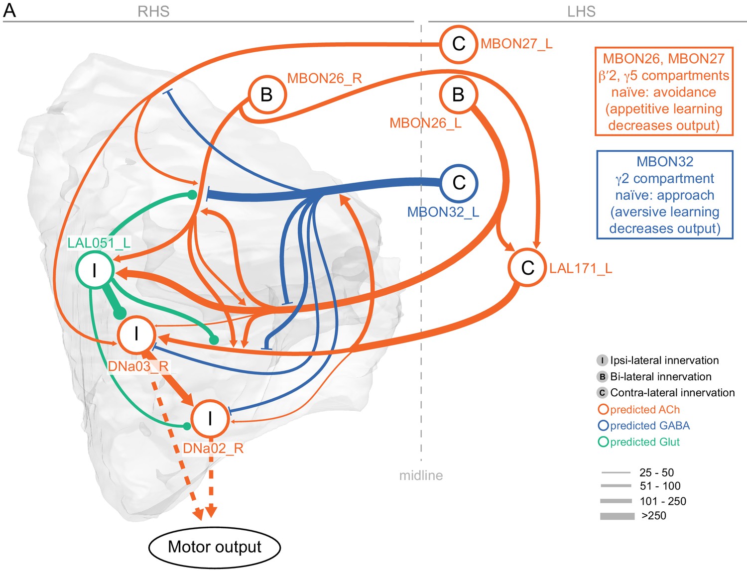
Multiple paths from atypical MBONs to DNs.
A simplified circuit diagram illustrating some of the prominent motifs used to connect atypical MBONs with the dendrites of DNs in the right hemisphere LAL. While several atypical MBONs synapse directly onto DNs, there are additional paths connecting atypical MBONs to DNs that are mediated by interneurons. Some interneurons, such as LAL051, are local, and others, such as LAL171, connect the right (RHS) and left (LHS) hemisphere LALs. Axo-axonal connections between MBONs and interneurons are common. These connections seem highly selective for two DNs cell types, DNa02 and DNa03, that are involved in steering the fly’s direction of movement: DNa03_R is MBON27’s third most highly connected output, MBON26’s 17th, LAL051_R’s second and LAL171_L’s third. While only about 15% of the DNs have so far been identified in the hemibrain v1.1 dataset, among those ~50 DN types only DNa03 and DNa02 receive significant input from the MBONs shown here. The atypical MBONs represent different types of sensory information, have different predicted behavioral valences and transmitters, and push-pull arrangements on shared targets are common. The GABAergic MBON32 has its dendrites in the γ2 compartment where it receives inputs from KCs representing both olfactory and visual sensory information (Figure 15 and Figure 25—figure supplement 1). The cholinergic MBON26 has its dendrites in the β′2 compartment where it receives inputs from KCs representing both olfactory and hygro/thermo sensory information (Figure 15 and Figure 25—figure supplement 1) and the cholinergic MBON27 has its inputs in the γ5 compartment where it receives inputs from KCs representing predominantly visual input (Figure 15 and Figure 25—figure supplement 1). MBONs 27 and 32 connect to the contralateral LAL and therefore only MBON 27_L and MBON32_L are shown, whereas MBON26 makes bilateral connections and both MBON26_L and MBON26_R are shown. LAL171_L receives about 20% of its total input from these two MBON types and then provides strong input to the contralateral DNa03. LAL051 gets over 15% of its input from left and right hemisphere MBON26s and also provides strong input to DNa03. DNa03 is strongly connected to DNa02, which promotes turning to the stimulated side (Rayshubskiy et al., 2020). Thus activity in MBON27 and MBON26 might promote avoidance by activating DNa03 in the contralateral LAL, causing steering away from a stimulus. Learning-related reductions in MBON26/27 activity would then promote approach. In general, the complexity of this circuitry, along with that of the atypical output network (as discussed in the text), further illustrates the highly integrative nature of the decision to turn. The synaptic inputs and outputs to LAL171_L were estimated using a combination of information from LAL171_L and LAL171_R to compensate for the incompleteness of the left hemisphere LAL in the hemibrain volume. See Figure 42—figure supplement 1 for the morphologies of LAL051 and LAL171.
Figure 42—figure supplement 1
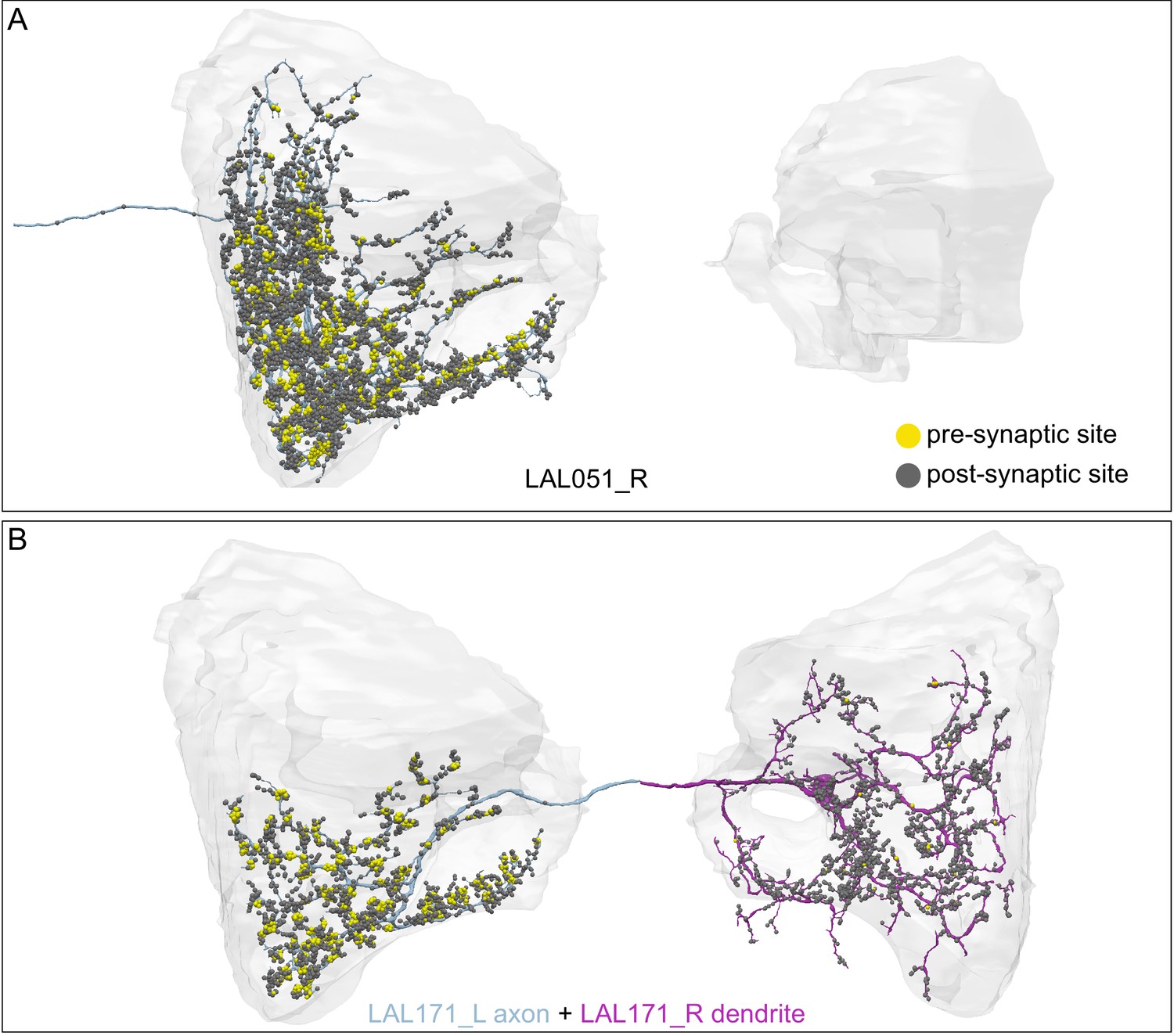
Morphologies of LAL051 and LAL171.
Presynaptic sites are shown as yellow dots and postsynaptic sites as gray dots. Because the left hemisphere LAL is incomplete in the hemibrain volume, the full morphology of LAL171 was constructed by using the LAL171_L axon and LAL171_R dendrite, as indicated. LAL051_R is a local interneuron with mixed polarity arbors confined to the right hemisphere LAL. LAL171 connects the LALs in the two hemispheres and is more highly polarized with predominantly postsynaptic sites in one LAL.
Additional files
-
Supplementary file 1
Constituents of each of the 402 PAM subtype clusters.
- https://cdn.elifesciences.org/articles/62576/elife-62576-supp1-v2.xlsx
-
Supplementary file 2
Constituents of each of the DAN input clusters shown in Figure 32.
- https://cdn.elifesciences.org/articles/62576/elife-62576-supp2-v2.xlsx
-
Transparent reporting form
- https://cdn.elifesciences.org/articles/62576/elife-62576-transrepform-v2.docx
Download links
A two-part list of links to download the article, or parts of the article, in various formats.
Downloads (link to download the article as PDF)
Open citations (links to open the citations from this article in various online reference manager services)
Cite this article (links to download the citations from this article in formats compatible with various reference manager tools)
The connectome of the adult Drosophila mushroom body provides insights into function
eLife 9:e62576.
https://doi.org/10.7554/eLife.62576


