Place-cell capacity and volatility with grid-like inputs
- Center for Theoretical and Computational Neuroscience, University of Texas, United States
- Department of Neuroscience, University of Texas, United States
- Department of Brain and Cognitive Sciences and McGovern Institute, MIT, United States
- Department of Mathematics and Neuroscience, The University of Texas, United States
Figures
Figure 1
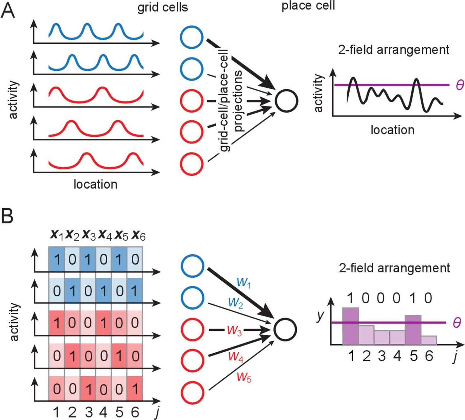
The grid-like code and modeling place cells as perceptrons.
(A) Grid-like inputs and a conceptual view of a place cell as a perceptron: each place cell combines its feedforward inputs, including periodic drive from grid cells (responses simplified here to one spatial dimension) of various periods and phases (blue and red cells are from modules with different periods) to generate location-specific activity that might be multiply peaked across large spaces. Can these place fields be arranged arbitrarily? (B) Idealization of a place cell as a perceptron: in discretized 1-D space, the grid-like inputs are discrete patterns that for simplicity we consider to be binary; place fields are assigned at locations where the weighted input sum exceeds a threshold . A place field arrangement can be considered as a set of binarized output labels (1 for each field, 0 for non-field locations) for the set of input patterns. We count field arrangements over the range of locations where the grid-like inputs have unique states; for two modules with periods , this range is 6 (the LCM of the grid periods). LCM = least common multiple; GCD = greatest common divisor.
Figure 2
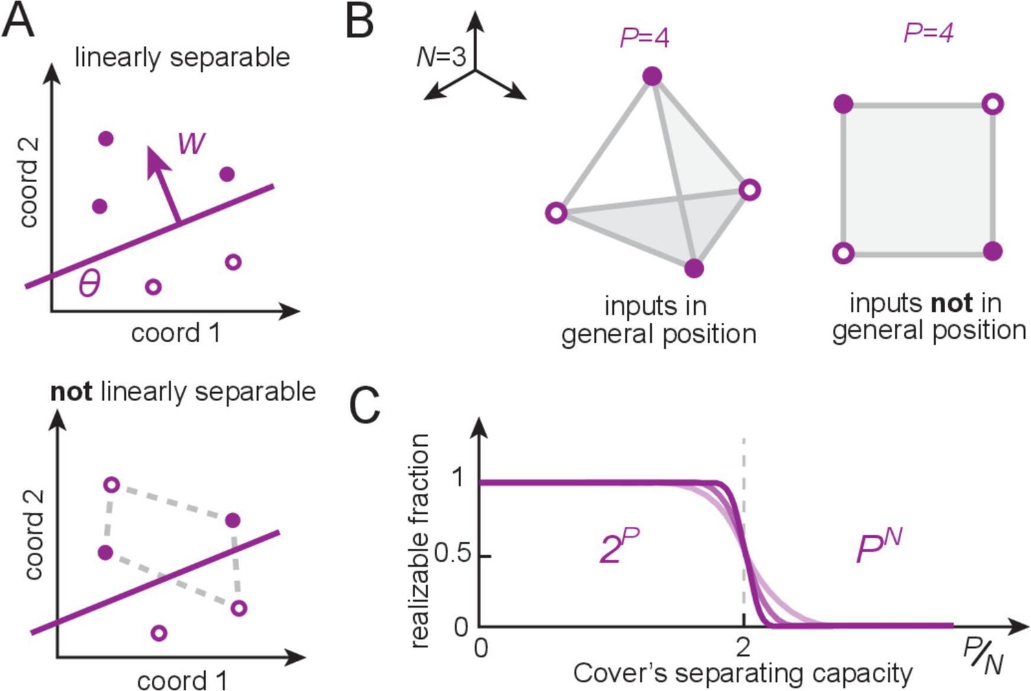
Linear separability, counting dichotomies, and separating capacity for perceptrons.
(A) A set of patterns (locations given by circles) that are assigned positive and negative labels (filled versus open), called a dichotomy of the patterns, is realizable by a perceptron if positive examples can be linearly separated (by a hyperplane) from the rest. The perceptron weights encode the direction normal to the separating hyperplane, and the threshold sets its distance from the origin. (B) An example with input dimension (the input dimension is the length of each input pattern vector, which equals the number of input neurons). When placed randomly, random real-valued patterns optimally occupy space and are said to be in general position (left); these patterns define a tetrahedron and all dichotomies are linearly separable. By contrast, structured inputs may occupy a lower-dimensional subspace and thus not lie in general position (right). This square configuration exhibits unrealizable dichotomies (as in A, bottom). (C) Cover’s results (Cover, 1965): for patterns in general position, the number of realizable dichotomies is , and thus the fraction of realizable dichotomies relative to all dichotomies is 1, when the number of patterns is smaller than the input dimension (). The fraction drops rapidly to zero when the number of patterns exceeds twice the input dimension (the separating capacity).
Figure 3
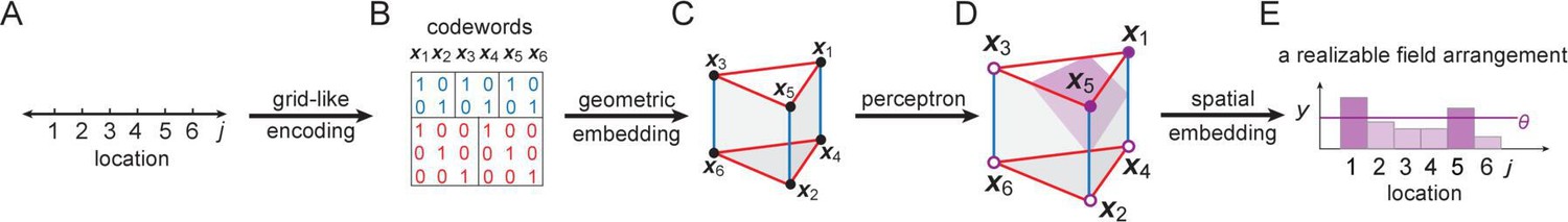
Our overall approach.
(A, B) Locations (indexed by ) map onto grid-like coding states (, defining the grid-like codebook) through the assignment of spatially periodic responses to grid cells, with different cells in a module having different phases and different modules having different periods. (This example: periods 2,3.) (C) The patterns in the grid-like codebook form some nonrandom, geometric structure. (D) The geometric structure defines which dichotomies are realizable by separating hyperplanes. (E) A realizable dichotomy in the abstract codebook pattern space, when mapped back to spatial locations, corresponds to a realizable field arrangement. Shown is a place field arrangement realized by the separating hyperplane from (D). Similarly, an unrealizable field arrangement can be constructed by examination of (D): it would consist of, for instance, fields at locations only (or, e.g., at only): vertices that cannot be grouped together by a single hyperplane.
Figure 4
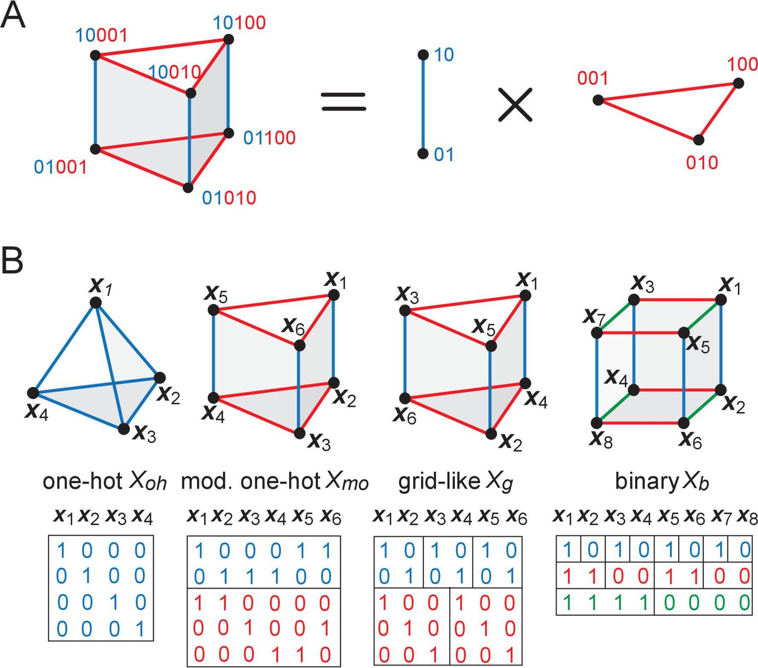
The geometry of structured inputs.
(A) Though the grid-like input patterns in the example Figure 1B are 5D, they have a simplified structure that can be embedded as a 3D triangular prism given by the product of a 2-graph (blue, middle) and 3-graph (red, right) because of the independently updating modular structure of the code. (B) Different codebooks and their geometries. At one end of the spectrum (left), one-hot codes consist of a single module; they are not hierarchical, and their geometry is always an elementary simplex (left). Grid cells and modular-one-hot codes (middle) have an intermediate level of hierarchy and consist of an orthogonal product of simplices. At the opposite end, the binary code (right) is the most hierarchical, consisting of as many modules as cells; the code has a hypercube geometry: vertices (codewords or patterns) on each face of the hypercube are far from being in general position.
Figure 5

Counting realizable place field arrangements.
(A) Geometric structure of a modular-one-hot code with two modules of periods and . (B–D) Because cells within a module can be freely permuted, we can arrange the cells in order of increasing weights and keep this ordering fixed during counting, without loss of generality. We arrange the cells in modules 1 and 2 along the ordinate and abcissa in increasing weight order (solid blue and red lines, respectively). Because the weights can all be assumed to be non-negative for modular-one-hot codes, the threshold can be interpreted as setting a summed-weight budget: no cell (weight) combinations (purple regions with purple-white circles) below the threshold (diagonal purple line) can contribute to a place field arrangement, while all cell combinations with larger summed weights (unmarked regions) can. Increasing the threshold (from B to C) decreases the number of permitted combinations, as does decreasing the weights (B to D). Weight changes (B, from solid to dashed lines) and threshold changes (C, solid to dashed line), so long as they do not change which lines are to the bottom-left of the threshold, do not affect the number of permitted combinations, reflecting the topological structure of the counting problem. (E) With Young diagrams (each corresponding to B–D above), we extract the purely topological part of the problem, stripping away analog weights to simplify counting. A Young diagram consists of stacks of blocks in rows of nonincreasing width within a grid of a maximum width and height. The number of realizable field arrangements is simply the total number and multiplicity of distinct Young diagrams that can be built of the given height and width (see Appendix 3), which in our case is given by the periods of the two modules.
Figure 6
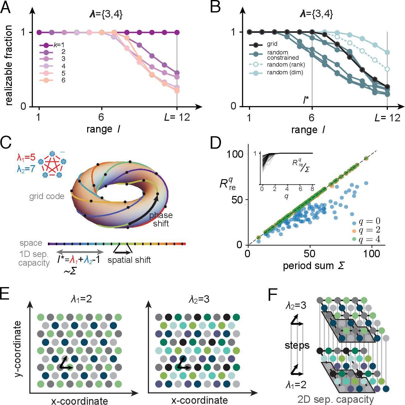
Place-cell-separating capacity.
(A) Fraction of K-field arrangements that are realizable with grid-like inputs as a function of range ( indicates the full range; in this example, grid periods are and ). (B) Fraction of realizable field arrangements (summed over ) as a function of range for grid cells (black); for random inputs, range refers to number of input patterns (solid cyan: random with matching input dimension; open/dashed cyan: random with input dimension equal to rank of the grid-like input matrix; dark teal: same as open cyan, but with weights constrained to be non-negative, as for grid-like inputs). With the non-negative weight constraint for random inputs, different specific input configurations produce quite different results, introducing considerable variability in separating capacity (unlike the unconstrained random input case or the grid code case for which results are exact rather than statistical). (C) The grid code is generated by iterated application of a phase-shift operator as a function of one-step updates in position over a contiguous 1D range. This feature of the code leads to a separating capacity that achieves its optimal value, given by the rank of the input matrix. (D) Separating capacity as a function of the sum of module periods for real-valued periods (randomly drawn from with , 100 realizations), showing the quality of the integer approximation at different resolutions. Integer approximations to the real-value periods at successively finer resolutions quickly converge, with results from and nearly indistinguishable from each other. Inset: ratio of separating capacity to sum of periods ( as a function of resolution quickly approaches 1 from below as increases). (E, F) Capacity results generalize to multidimensional spatial settings: (E) in 2D, grid-cell-activity patterns lie on a hexagonal lattice (all circles of one color mark the activity locations of one grid cell). For grid periods , this code utilizes 4 two-periodic cells and 9 three-periodic cells, respectively. (F) Full range of the 2D grid-like code from (E). The set of contiguous locations over which any place field arrangement is realizable (the 2D separating capacity) is shown in gray.
Figure 7
Robustness of place field arrangements to noise and nongrid inputs.
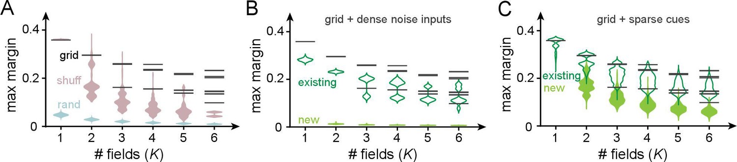
In (A–C), grid periods are ; the number of input patterns is set to for all input codes. Input patterns are normalized to have unity L1 norm in all cases. Maximum margins are determined by using SVC in scikit-learn (Pedregosa et al., 2011) (with thresholds and no weight constraints). (A) Black bars: the maximum margins of all realizable arrangements with grid-like inputs (bars have high multiplicity: across the very large number of realizable field arrangements, the set of distinct maximum margins is small and discrete because of the regular geometric structure of the grid-like code). Pink: margins for shuffled grid inputs that break the code’s modularity (shuffling neurons across modules for each pattern; 10 shuffles per and sampling 1000 realizable field arrangements per shuffle). Blue: margins for random inputs in general position (inputs sampled i.i.d. uniformly from ; 10 realizations of a random matrix per , 1000 realizable field arrangements sampled per realization). (B) Effect of noise on margins. We added dense noise inputs (100 non-negative i.i.d. random inputs at each location) to the place cell, in addition to the 74 grid-like inputs. (The expected value of each random input was 20% of the population mean of the grid inputs; thus, the summed random input was on average the size of the summed grid input.) Black: noise-free margins as in (A). Empty green violins: margins of existing field arrangements modestly shrink in size. Solid green violins: margins of some newly created field arrangements: these are small and thus unstable. (C) Effect of sparse spatial inputs (plots as in C). (We added 100 sparse inputs per location; each sparse input had fields placed randomly across the full range , so that the summed sparse input was on average the size of the summed grid input. The combined grid and nongrid input at each location was normalized to 1.)
Figure 8
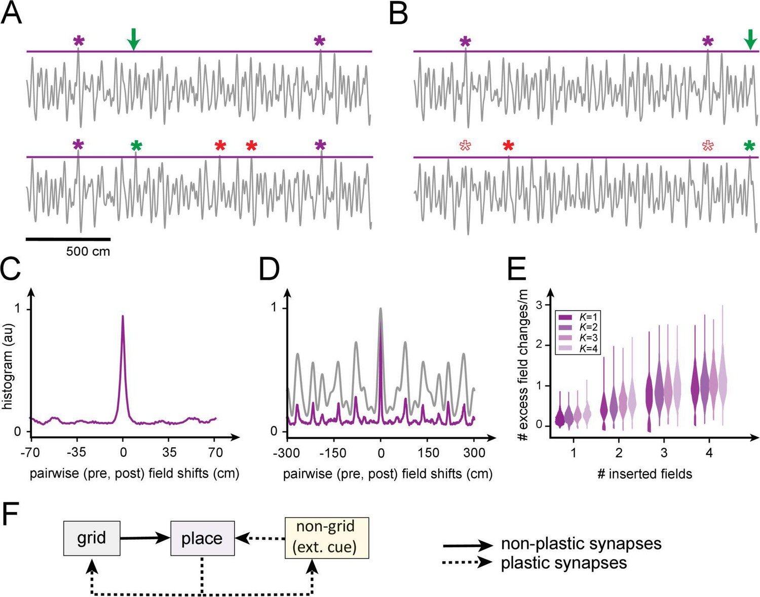
Predicted volatility of place field arrangements.
(A) Top: original field arrangement over a 20 m space (gray line: summed inputs to place cell; purple stars: original field locations; green arrow: location where new field will be induced by Hebbian plasticity in grid-place weights). Bottom: after induction of the new field (green star), two new uncontrolled fields appear (red stars). (B) Similar to (A): the insertion of a new field at a random location (green star) leads to one uncontrolled new field (red star) and the loss of two original fields (empty red stars). (C) Histogram of changes, after single-field insertion, in pairwise inter-field intervals (spacings): the primary off-target effect of field insertion is for other fields to appear or disappear, but existing fields do not tend to move. (D) A spatially extended version of (C) (purple), together with the (vertically rescaled) autocorrelation of the grid inputs to the cell (gray): new fields tend to appear at spacings corresponding to peaks in the input autocorrelation function. (E) Sum of uncontrolled field insertions or deletions per meter, in response to inserted fields when starting with a K-field arrangement over 20 m. (F) High place field volatility resulting from plasticity in the grid-to-place synapses suggests the possibility that grid-place weights might be relatively rigid (nonplastic).
Appendix 1—figure 1
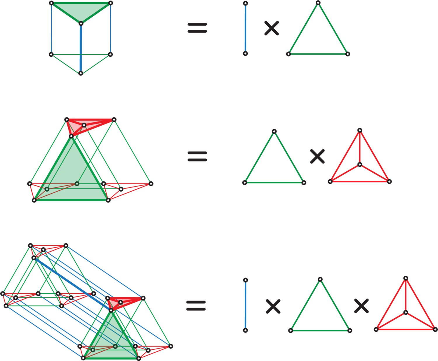
Simplicial decomposition.
The convex hull generated by the grid code activity patterns is a product of simplices.
Appendix 2—scheme 1
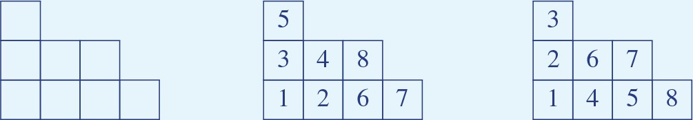
Examples of Young tableaux.
Appendix 2—figure 1
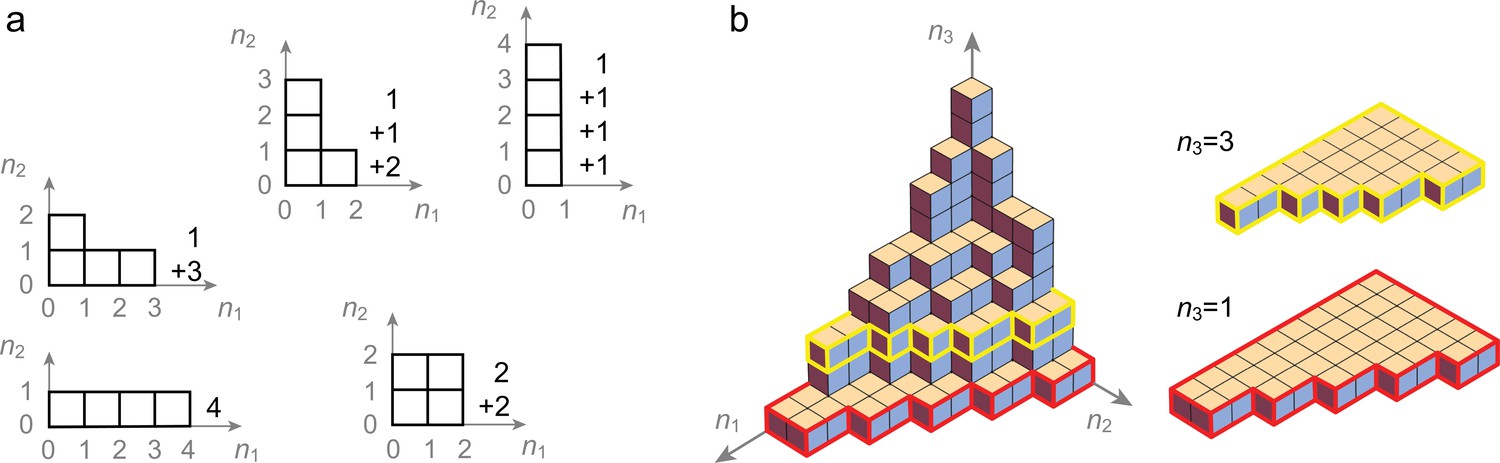
Multidimensional Young diagrams.
a. Lattice representations of the 2-dimensional Young diagrams of size 4, depicting the integer partitions of 4. b. Lattice representation of a 3-dimensional Young diagram with two 2-dimensional Young diagrams defined as horizontal restrictions.
Appendix 2—figure 2
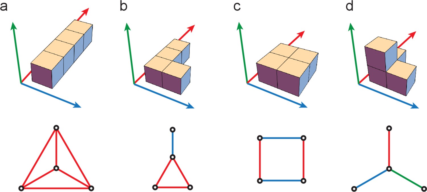
Linearly separable 4-dichotomies.
Top: there are four possible Young diagrams a, b, c, and d, of size 4, spanning at most three dimensions. Lattice points lying along the mth dimension represent grid-like inputs in whose coordinates only differ in the mth module. Bottom: Graphical edge structure arising from embedding a Young diagram within , the convex polytope defined by grid-like inputs.
Appendix 2—figure 3

Counting 2-module Young diagram.
Linearly separable dichotomies (left panel) can be associated to a unique Young diagram (middle panel). These Young diagrams are entirely specified by their frontier path, separating active positions from inactive ones. Enumerating all possible frontier paths allows one to count all the linearly separable dichotomies for two modules.
Appendix 3—figure 1
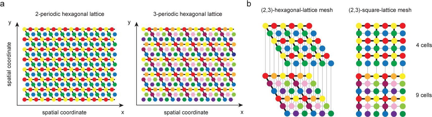
Hexagonal and square lattice in two dimensions.
(a) In two dimensions, 2-periodic and 3-periodic modules comprise respectively four and nine possible grid-cell-activity pattern. For instance, red, green, blue, and yellow patterns in the leftmost lattice correspond to the four possible patterns of activity that a 2-periodic cell can exhibit on an hexagonal lattice. (b) The maximum lattice mesh over which each position is uniquely encoded by the grid-like code is given as . Moreover, the hexagonal symmetry plays no role in our capacity calculations and one can consider a square lattice of positions instead.
Tables
Table 1
Number and fraction of realizable dichotomies with binary, modular-one-hot ( modules) and one-hot input codes with the same input cell budget ().
| # cells | # input patts (L) | # lin dichot | Frac lin dichot | |
|---|---|---|---|---|
| Binary | 2λ | 22λ | 22λ2 | |
| = | << | << | >> | |
| Modular-one-hot | 2λ | λ2 | ||
| = | << | << | >> | |
| One-hot | 2λ | 2λ | 22λ | 1 |
Additional files
Download links
A two-part list of links to download the article, or parts of the article, in various formats.
Downloads (link to download the article as PDF)
Open citations (links to open the citations from this article in various online reference manager services)
Cite this article (links to download the citations from this article in formats compatible with various reference manager tools)
Place-cell capacity and volatility with grid-like inputs
eLife 10:e62702.
https://doi.org/10.7554/eLife.62702


