A new model of decision processing in instrumental learning tasks
- University of Amsterdam, Department of Psychology, Netherlands
- Leiden University, Department of Psychology, Netherlands
- University of Newcastle, School of Psychology, Australia
Figures
Figure 1

Comparison of the decision-making models.
Bottom graphs visualize how Q-values are linked to accumulation rates. Top panel illustrates the evidence-accumulation process of the DDM (panel A) and racing diffusion (RD) models (panels B and C). Note that in the race models there is no lower bound. Equations 2–4 formally link Q-values to evidence-accumulation rates. In the RL-DDM, the difference in Q-values is accumulated, weighted by free parameter , plus additive within-trial white noise W with standard deviation . In the RL-RD, the (weighted) Q-values for both choice options are independently accumulated. An evidence-independent baseline urgency term, (equal for all accumulators), further drives evidence accumulation. In the RL-ARD models, the advantages in Q-values are accumulated as well, plus the evidence-independent baseline term . The gray icons indicate the influence of the Q-value sum on evidence accumulation, which is not included in the limited variant of the RL-ARD. In all panels, bold-italic faced characters indicate parameters. Q1 and Q2 are Q-values for both choice options, which are updated according to a delta learning rule (Equation 1 at the bottom of the graph), with learning rate .
Figure 2
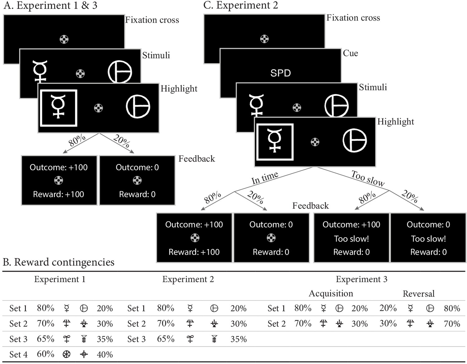
Paradigms for experiments 1–3.
(A) Example trial for experiments 1 and 3. Each trial starts with a fixation cross, followed by the presentation of the stimulus (until choice is made or 2.5 s elapses), a brief highlight of the chosen option, and probabilistic feedback. Reward probabilities are summarized in (B). Percentages indicate the probabilities of receiving +100 points for a choice (with 0 otherwise). The actual symbols used differed between experiments and participants. In experiment 3, the acquisition phase lasted 61–68 trials (uniformly sampled each block), after which the reward contingencies for each stimulus set reversed. (C) Example trial for experiment 2, which added a cue prior to each trial (‘SPD’ or ‘ACC’), and had feedback contingent on both the choice and choice timing. In the SPD condition, RTs under 600 ms were considered in time, and too slow otherwise. In the ACC condition, choices were in time as long as they were made in the stimulus window of 1.5 s. Positive feedback ‘Outcome: +100’ and ‘Reward: +100’ were shown in green letters, negative feedback (‘Outcome: 0’, ‘Reward: 0’, and ‘Too slow!”) were shown in red letters.
Figure 3 with 4 supplements
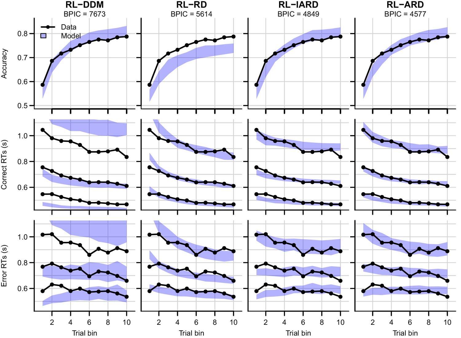
Comparison of posterior predictive distributions of the four RL-EAMs.
Data (black) and posterior predictive distribution (blue) of the RL-DDM (left column), RL-RD, RL-lARD, and RL-ARD (right column). Top row depicts accuracy over trial bins. Middle and bottom row show 10th, 50th, and 90th RT percentiles for the correct (middle row) and error (bottom row) response over trial bins. Shaded areas correspond to the 95% credible interval of the posterior predictive distributions. All data are collapsed across participants and difficulty conditions.
Figure 3—figure supplement 1

Comparison of posterior predictive distributions of four additional RL-DDMs.
Data are black dots and lines, posterior predictive distribution are blue. Top row depicts accuracy over trial bins. Middle and bottom row illustrate 10th, 50th, and 90th quantile RT for the correct (middle row) and error (bottom row) response over trial bins. Shaded areas correspond to the 95% credible interval of the posterior predictive distributions. All data are collapsed across participants and difficulty conditions. The summed BPICs were 7717 (RL-DDM A1), 7636 (RL-DDM A2), 4844 (RL-DDM A3) and 4884 (RL-DDM A4). Hence, the largest improvement of quality of fit of the RL-DDM was obtained by adding .
Figure 3—figure supplement 2
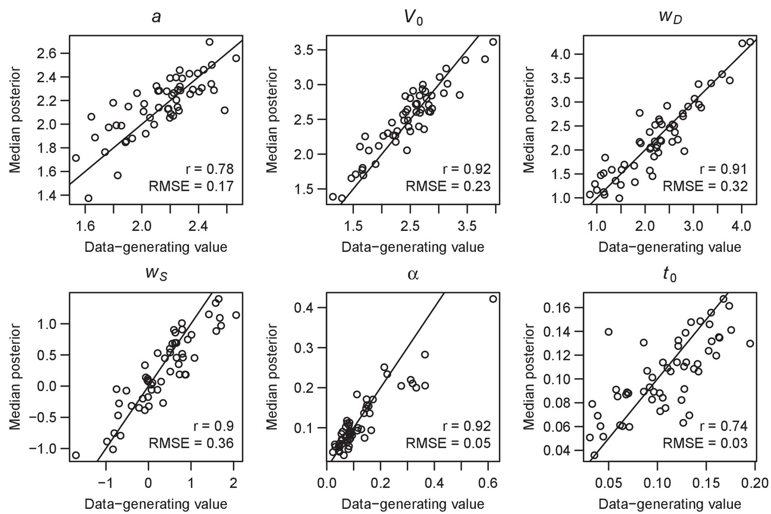
Parameter recovery of the RL-ARD model, using the experimental paradigm of experiment 1.
Parameter recovery was done by first fitting the RL-ARD model to the empirical data, and then simulating the exact same experimental paradigm (208 trials, 55 subjects, four difficulty conditions) using the median parameter estimates obtained from the model fit. Subsequently, the RL-ARD was fit to the simulated data. The recovered median posterior estimates (y-axis) are plotted against the data-generating values (x-axis). Pearson’s correlation coefficient r and the root mean square error (RMSE) are shown in each panel. Diagonal lines indicate the identity x = y.
Figure 3—figure supplement 3
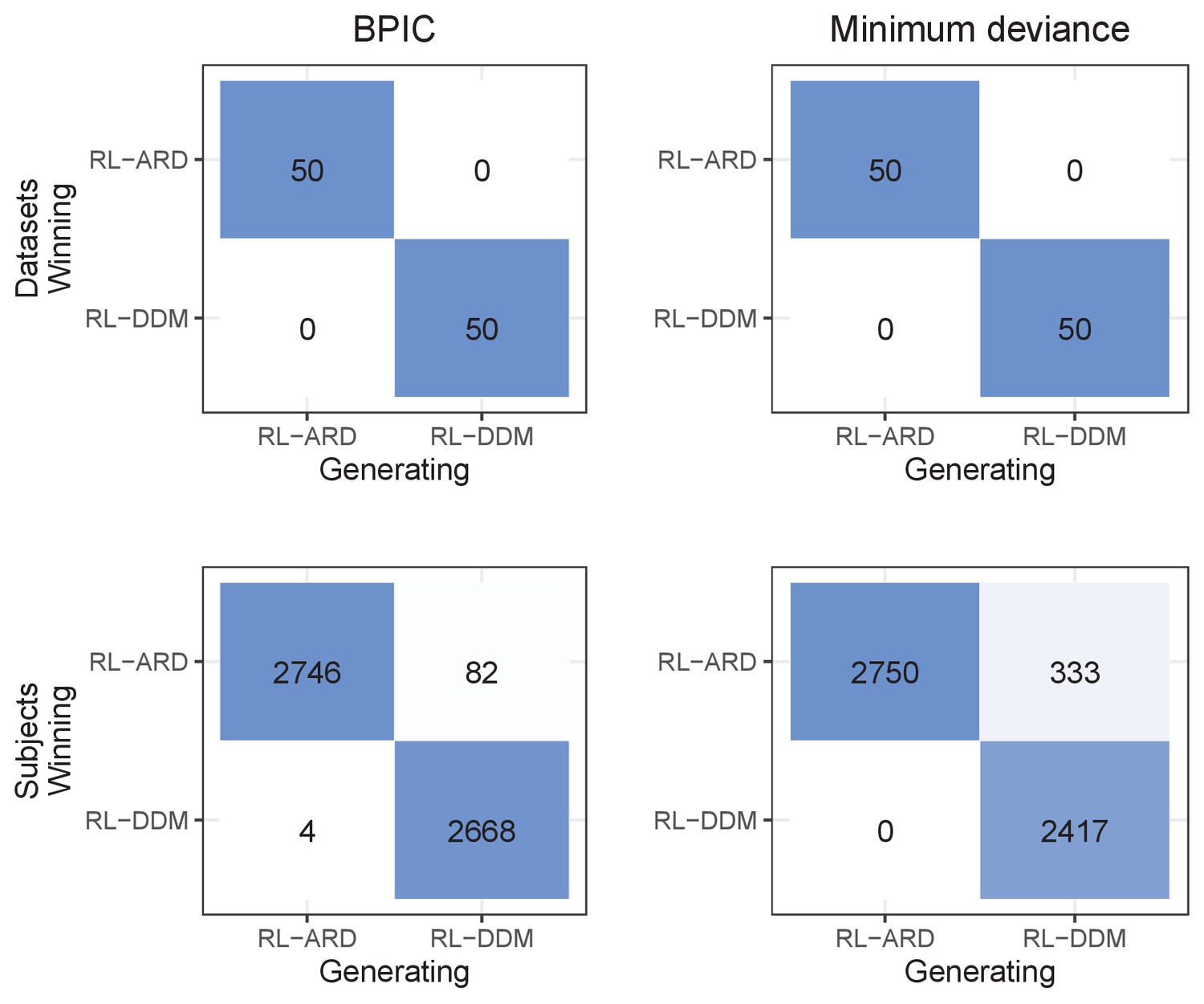
Confusion matrices showing model separability.
Here, we first fit the RLDDM and RL-ARD to the empirical data of experiment 1, and then simulating 50 full datasets with both models using the exact same experimental paradigm (208 trials, 55 subjects, 4 difficulty conditions), and using the median parameter estimates obtained from the model fits. Hence, in total 100 full datasets (5500 subjects) were simulated. We then fit both the RL-DDM and RL-ARD to all 100 simulated datasets. The matrices visualize the model confusability when using the BPIC (left column) or minimum deviance (right column) as a model comparison metric. The minimum deviance is a measure of quality of fit without a penalty for model complexity. The top row shows the model comparisons per dataset (using the summed BPIC / minimum deviances), bottom row shows the model comparisons per subject. Model comparisons using the BPIC perfectly identified the data-generating model when summing BPICs across subjects. By subject individually, the RL-ARD incorrectly won model comparisons for 82 subjects (3%); the RL-DDM incorrectly won for 4 subjects (0.1%). Interestingly, when using the summed minimum deviances as a model comparison metric (thus not penalizing for model complexity), the across-subject model comparisons perfectly identified the data-generating model. By subject individually, the RL-ARD incorrectly won comparisons for 333 subjects (12%). Combined, this indicates that the RL-ARD, while more complex, is generally not sufficiently flexible to outperform RL-DDM in terms of the quality of fit on data generated by the RL-DDM.
Figure 3—figure supplement 4
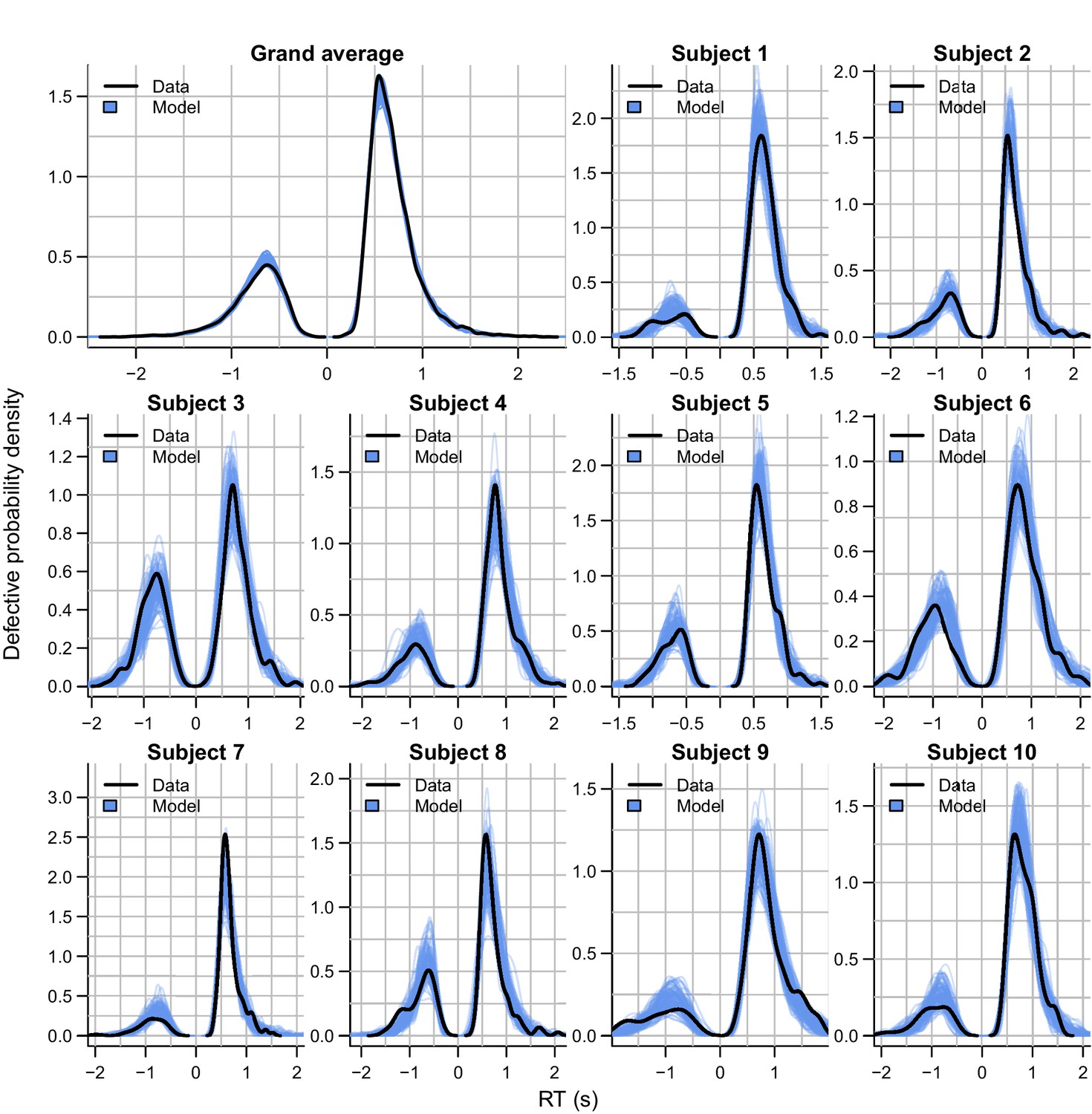
Empirical (black) and posterior predictive (blue) defective probability densities of the RT distributions estimated using kernel density approximation.
The error RT distributions are shown as negative RTs for visualization. Blue lines represent 100 posterior predictive RT distributions from the RL-ARD model. The grand average is the RT distribution across all trials and subjects, subject-wise RT distributions are across all trials per subject for the first ten subjects, for which the quality of fit was representative for the entire dataset.
Figure 4 with 4 supplements
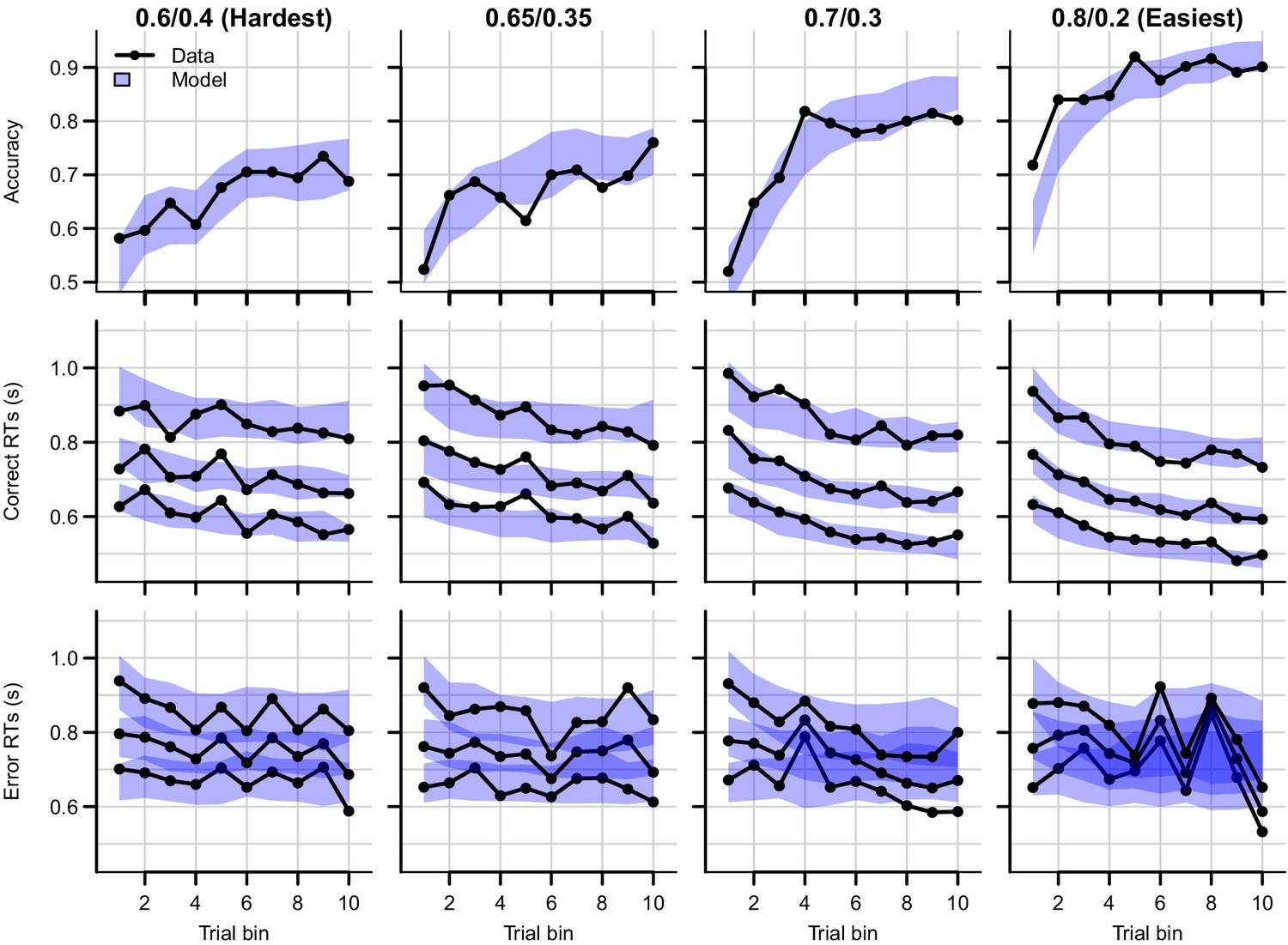
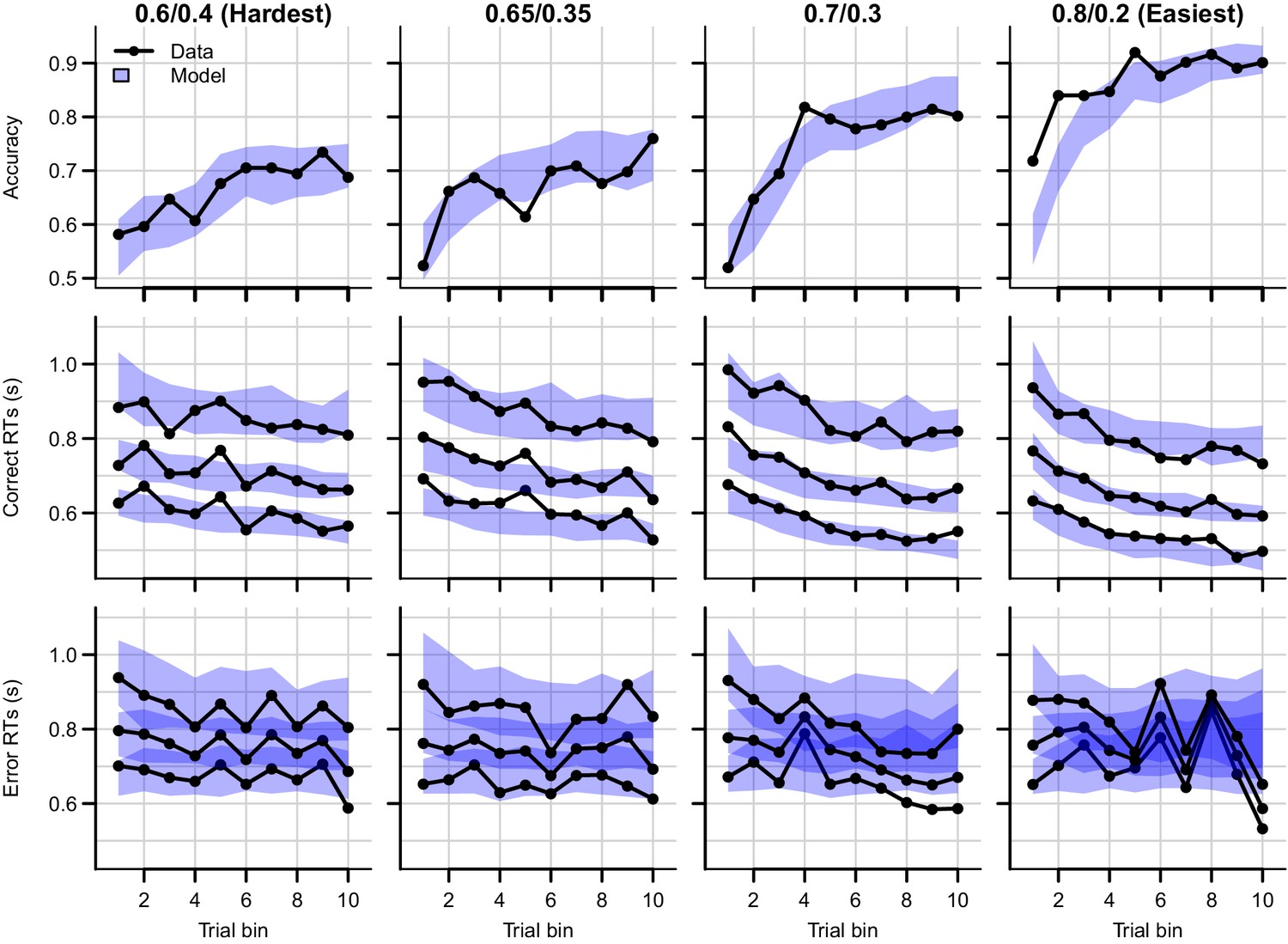
Data (black) and posterior predictive distribution of the RL-ARD (blue), separately for each difficulty condition.
Column titles indicate the reward probabilities, with 0.6/0.4 being the most difficult, and 0.8/0.2 the easiest condition. Top row depicts accuracy over trial bins. Middle and bottom rows show 10th, 50th, and 90th RT percentiles for the correct (middle row) and error (bottom row) response over trial bins. Shaded areas correspond to the 95% credible interval of the posterior predictive distributions. All data and fits are collapsed across participants.
Figure 4—figure supplement 1
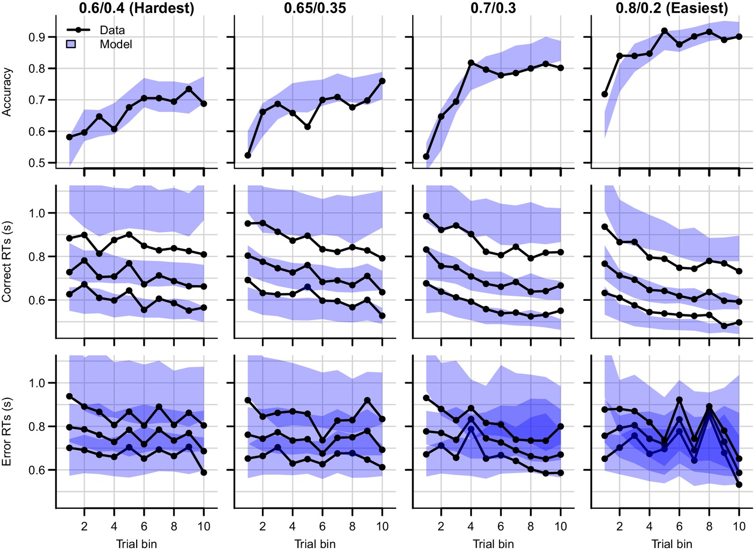
Data (black) and posterior predictive distribution of the RL-DDM (blue), separately for each difficulty condition.
Row titles indicate the reward probabilities, with 0.6/0.4 being the most difficult, and 0.8/0.2 the easiest condition. Top row depicts accuracy over trial bins. Middle and bottom row illustrate 10th, 50th, and 90th quantile RT for the correct (middle row) and error (bottom row) response over trial bins. Shaded areas correspond to the 95% credible interval of the posterior predictive distributions. All data are collapsed across participants.
Figure 4—figure supplement 2
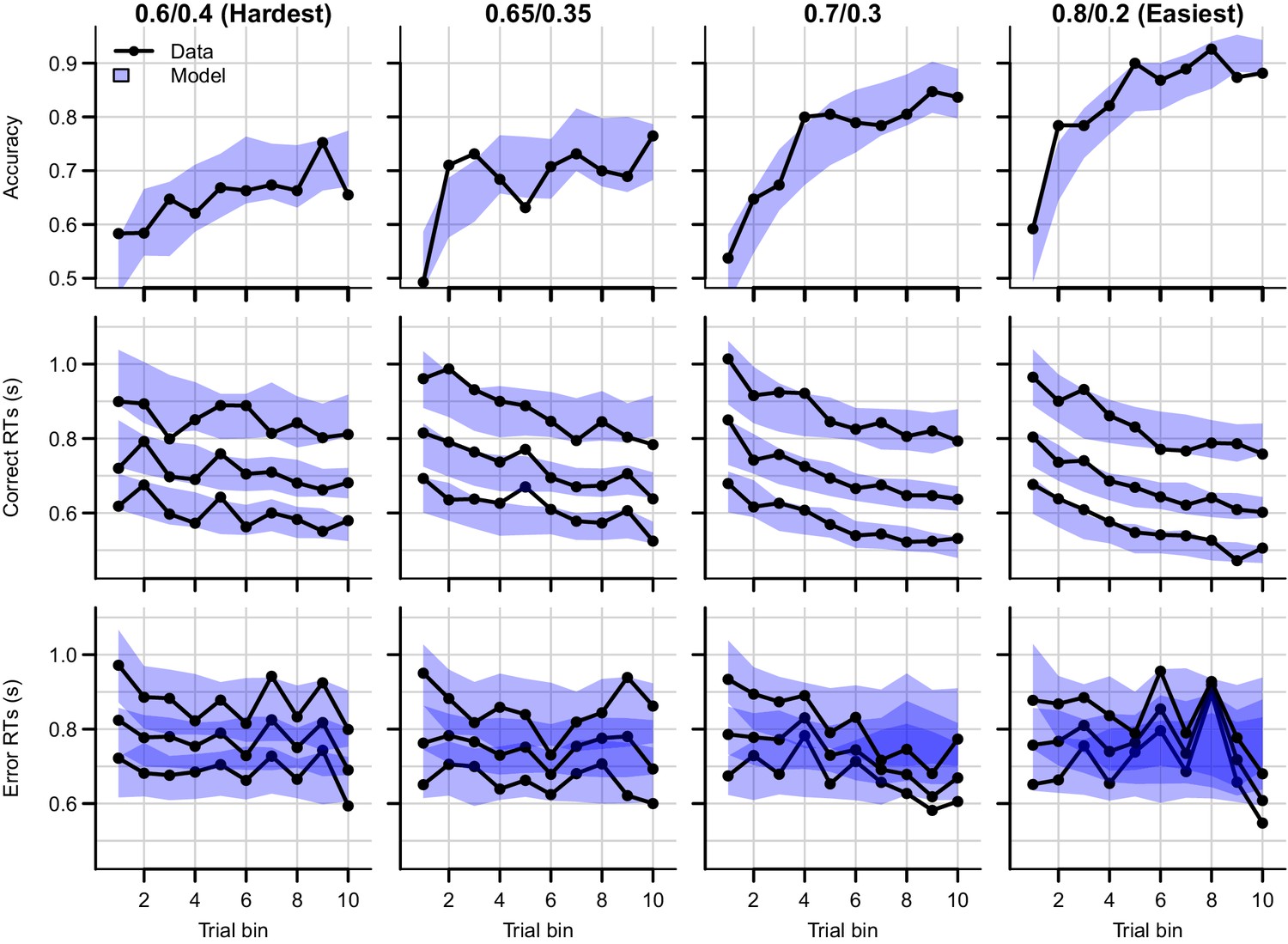
Data (black) and posterior predictive distribution of the RL-ARD (blue), separately for each difficulty condition, excluding 17 subjects which had perfect accuracy in the first bin of the easiest condition.
Row titles indicate the reward probabilities, with 0.6/0.4 being the most difficult, and 0.8/0.2 the easiest condition. Top row depicts accuracy over trial bins. Middle and bottom row illustrate 10th, 50th, and 90th quantile RT for the correct (middle row) and error (bottom row) response over trial bins. Shaded areas correspond to the 95% credible interval of the posterior predictive distributions. All data are collapsed across participants.
Figure 4—figure supplement 3
Posterior predictive distribution of the RL-ALBA model on the data of experiment 1, with one column per difficulty condition.
The LBA assumes that, on every trial, two accumulators race deterministically toward a common bound b. Each accumulator i starts at a start point sampled from a uniform distribution [0, A], and with a speed of evidence accumulation sampled from a normal distribution . In the RL-ALBA model, we used Equation 4 to link Q-values to LBA drift rates and (excluding the term, since the LBA assumes no within-trial noise). Instead of directly estimating threshold b, we estimated the difference B = b-A (which simplifies enforcing b>A). We used the following mildly informed priors for the hypermeans: , truncated at lower bound 0, , , , truncated at lower bound 0, and , truncated at lower bound 0.025 and upper bound 1. For the hyperSDs, all priors were . The summed BPIC was 4836, indicating that the RL-ALBA performs slightly better than the RL-DDM with between-trial variabilities (BPIC = 4844), and better than the RL-lARD (BPIC = 4849), but not as well as the RL-ARD (BPIC = 4577).
Figure 4—figure supplement 4
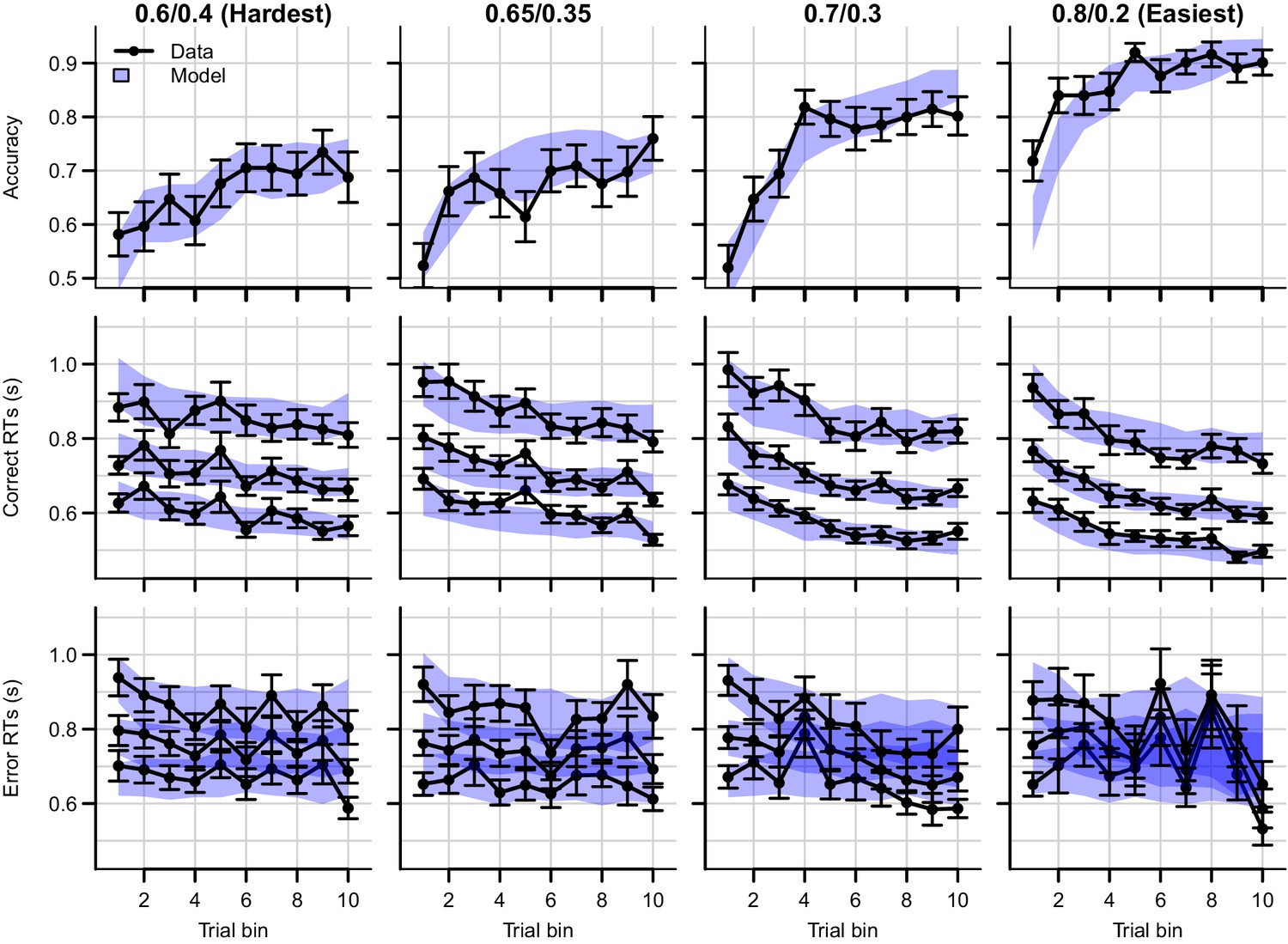
Data (black) and posterior predictive distribution of the RL-ARD (blue), separately for each difficulty condition.
Column titles indicate the reward probabilities, with 0.6/0.4 being the most difficult, and 0.8/0.2 the easiest condition. Top row depicts accuracy over trial bins. Middle and bottom rows show 10th, 50th, and 90th RT percentiles for the correct (middle row) and error (bottom row) response over trial bins. Shaded areas correspond to the 95% credible interval of the posterior predictive distributions. All data and fits are collapsed across participants. Error bars depict standard errors.
Figure 5
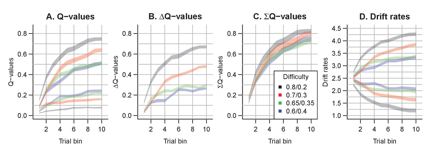
The evolution of Q-values and their effect on drift rates in the RL-ARD.
A depicts raw Q-values, separate for each difficulty condition (colors). B and C depict the Q-value differences and the Q-value sums over time. The drift rates (D) are a weighted sum of the Q-value differences and Q-value sums, plus an intercept.
Figure 6 with 5 supplements
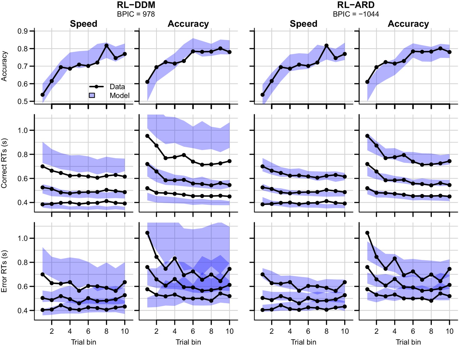
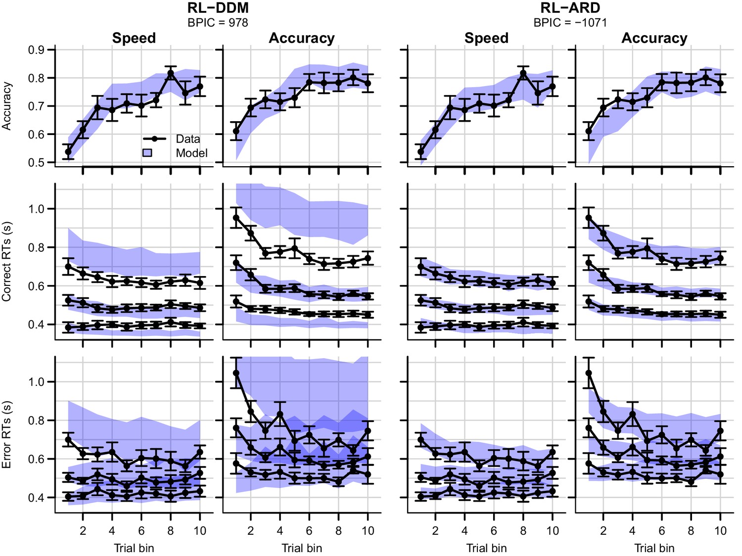
Data (black) and posterior predictive distributions (blue) of the best-fitting RL-DDM (left columns) and the winning RL-ARD model (right columns), separate for the speed and accuracy emphasis conditions.
Top row depicts accuracy over trial bins. Middle and bottom row show 10th, 50th, and 90th RT percentiles for the correct (middle row) and error (bottom row) response over trial bins. Shaded areas in the middle and right column correspond to the 95% credible interval of the posterior predictive distribution.
Figure 6—figure supplement 1
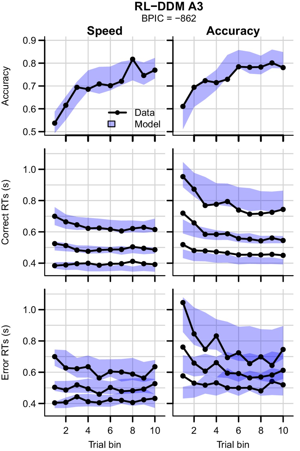
Data (black) of experiment 2 and posterior predictive distribution (blue) of the RL-DDM A3 with separate thresholds for the SAT conditions, and between-trial variabilities in drift rates, start points, and non-decision times.
The corresponding summed BPIC was -861, an improvement over the RL-DDM, but outperformed by the RL-ARD ( in favor of the RL-ARD). Top row depicts accuracy over trial bins. Middle and bottom row illustrate 10th, 50th, and 90th quantile RT for the correct (middle row) and error (bottom row) response over trial bins. Left and right column are speed and accuracy emphasis condition, respectively. Shaded areas correspond to the 95% credible interval of the posterior predictive distributions.
Figure 6—figure supplement 2
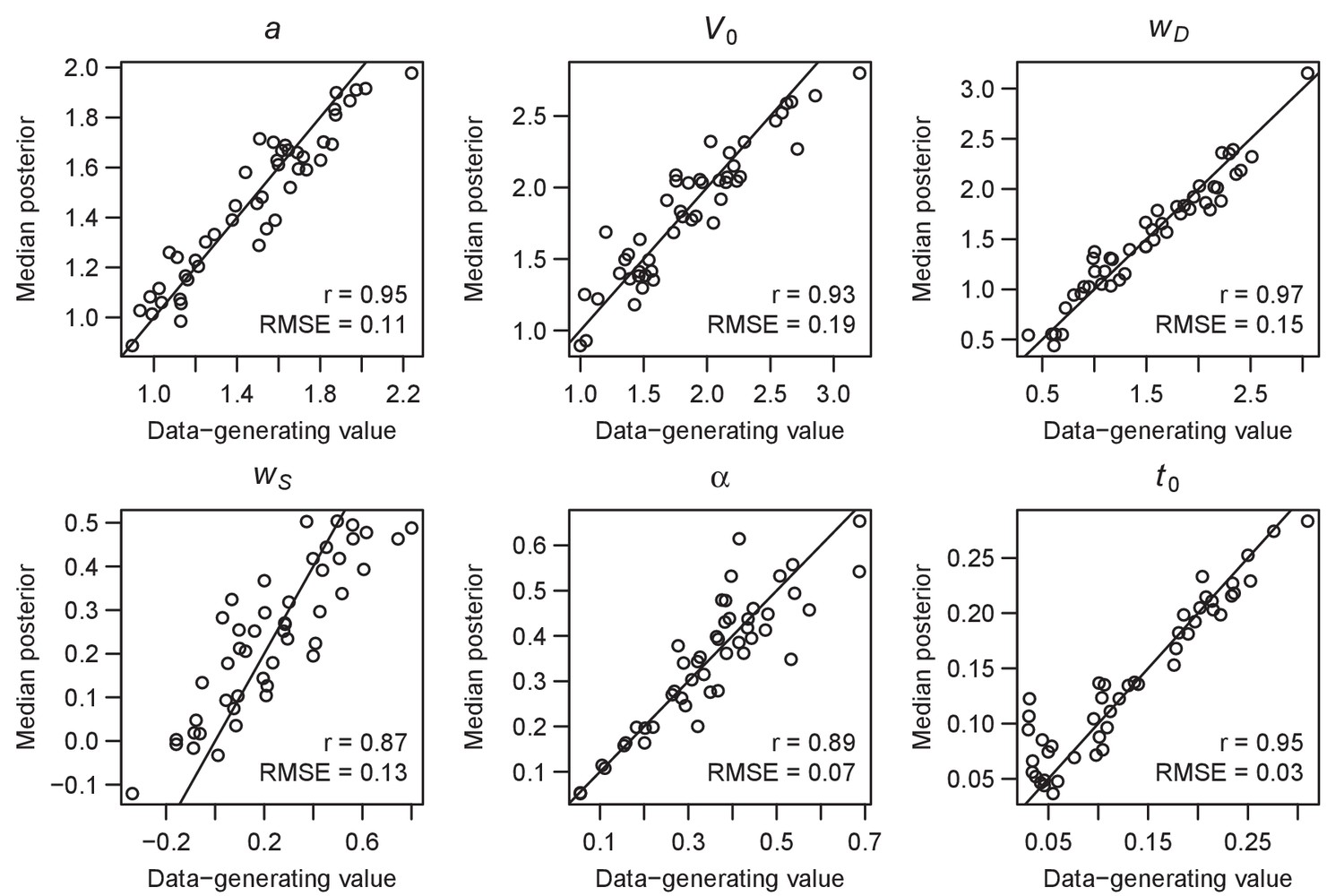
Parameter recovery of the RL-ARD model, using the experimental paradigm of experiment 2.
Parameter recovery was done by first fitting the RL-ARD model to the empirical data, and then simulating the exact same experimental paradigm (19 subjects, three difficulty conditions, 2 SAT conditions, 312 trials) using the median parameter estimates obtained from the model fit. Subsequently, the RL-ARD was fit to the simulated data. The median posterior estimates (y-axis) are plotted against the data-generating values (x-axis). Pearson’s correlation coefficient r and the root mean square error (RMSE) are shown in each panel. Diagonal lines indicate the identity x = y.
Figure 6—figure supplement 3

Mean RT (left column) and choice accuracy (right column) across trial bins (x-axis) for experiments 2 and 3 (rows).
Block numbers are color-coded. Error bars are 1 SE. Mixed effects models indicated that in experiment 2, RTs decreased with block number (b = −0.04, SE = 6.15*10−3, 95% CI [−0.05,–0.03], p = 6.61*10−10) as well as with trial bin (b = −0.02, SE = 2.11*10−3, 95% CI [−0.02,–0.01], p = 1.68*10−13), and there was an interaction between trial bin and block number (b = 3.61*10−3, SE = 9.86*10−4, 95% CI [0.00, 0.01], p = 2.52*10−4). There was a main effect of (log-transformed) trial bin on accuracy (on a logit scale; b = 0.36, SE = 0.11, 95% CI [0.15, 0.57], p = 7.99*10−4), but no effect of block number, nor an interaction between block number and trial bin on accuracy. In experiment 3, response times increased with block number (b = 0.02, SE = 3.10*10−3, 95% CI [0.01, 0.02], p = 1.21*10−7), decreased with trial bin (b = −4.24*10−3, SE = 1.37*10−3, 95% CI [−6.92*10−3, −1.56*10−3], p = 0.002), but there was no interaction between trial bin and block number (b = −9.15*10−4, SE = 5*10−4, 95% CI [0.00, 0.00], p = 0.067). The bottom left panel suggests that the main effect of block number on RT is largely caused by an increase in RT after the first block. Accuracy decreased with (log-transformed) trial bin (on a logit scale: b = −0.12, SE = 0.05, 95% CI [−0.22,–0.02], p = 0.02), decreased with block number (b = −0.08, SE = 0.03, 95% CI [−0.14,–0.02], p = 0.009), but there was no interaction (b = 0.02, SE = 0.02, 95% CI [−0.02, 0.06], p = 0.276). The decrease in accuracy with trial bin is expected due to the presence of reversals. The combination of an increase in RT and a decrease in accuracy after the first block could indicate that participants learnt the structure of the task (i.e. the presence of reversals) in the first block, and adjusted their behavior accordingly. In line with this speculation, the accuracy in trial bin 6 (in which the reversal occurred) was lowest in the first block, which suggests that participants adjusted to the reversal faster in the later blocks. In experiment 4, response times decreased with block number (b = −0.04, SE = 9.08*10−3, 95% CI [−0.06,–0.02], p = 3.19*10−3) and there was an interaction between block number and trial bin (b = −4.31*10−3, SE = 1.45*10−3, 95% CI = [−0.01, 0.00], p = 0.003), indicating that the decrease of RTs over trial bins was larger for the later blocks. There was no main effect of trial bin on RTs. There was a main effect of (log-transformed) trial bin on accuracy (on a logit scale: b = 0.60, SE = 0.07, 95% CI [0.47, 0.73], p < 10-16), but no main effect of block and no interaction between block and trial bin.
Figure 6—figure supplement 4
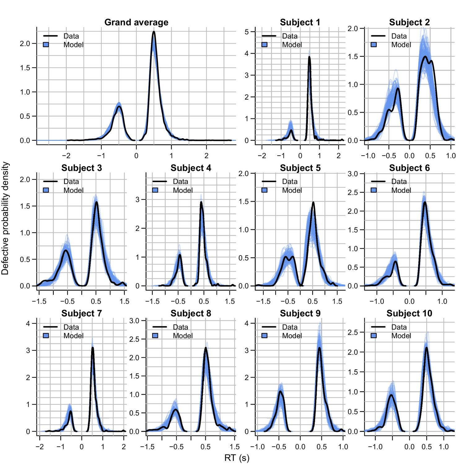
Empirical (black) and posterior predictive (blue) defective probability densities of the RT distributions of experiment 2, estimated using kernel density approximation.
Negative RTs correspond to error RTs. Blue lines represent 100 posterior predictive RT distributions from the RL-ARD model. The grand average is the RT distribution across all trials and subjects, subject-wise RT distributions are across all trials per subject for the first 10 subjects, for which the quality of fit was representative for the entire dataset.
Figure 6—figure supplement 5
Data (black) and posterior predictive distributions (blue) of the best-fitting RL-DDM (left columns) and the winning RL-ARD model (right columns), separate for the speed and accuracy emphasis conditions.
Top row depicts accuracy over trial bins. Middle and bottom row show 10th, 50th, and 90th RT percentiles for the correct (middle row) and error (bottom row) response over trial bins. Shaded areas in the middle and right column correspond to the 95% credible interval of the posterior predictive distribution. Error bars depict standard errors.
Figure 7 with 5 supplements
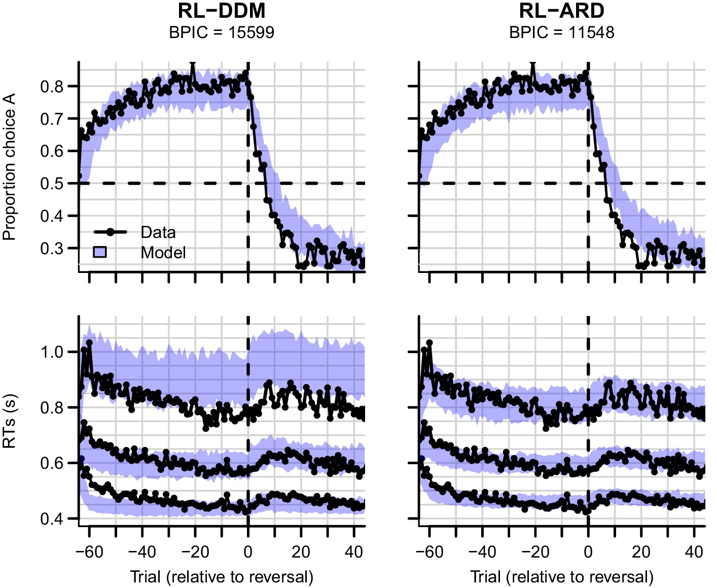
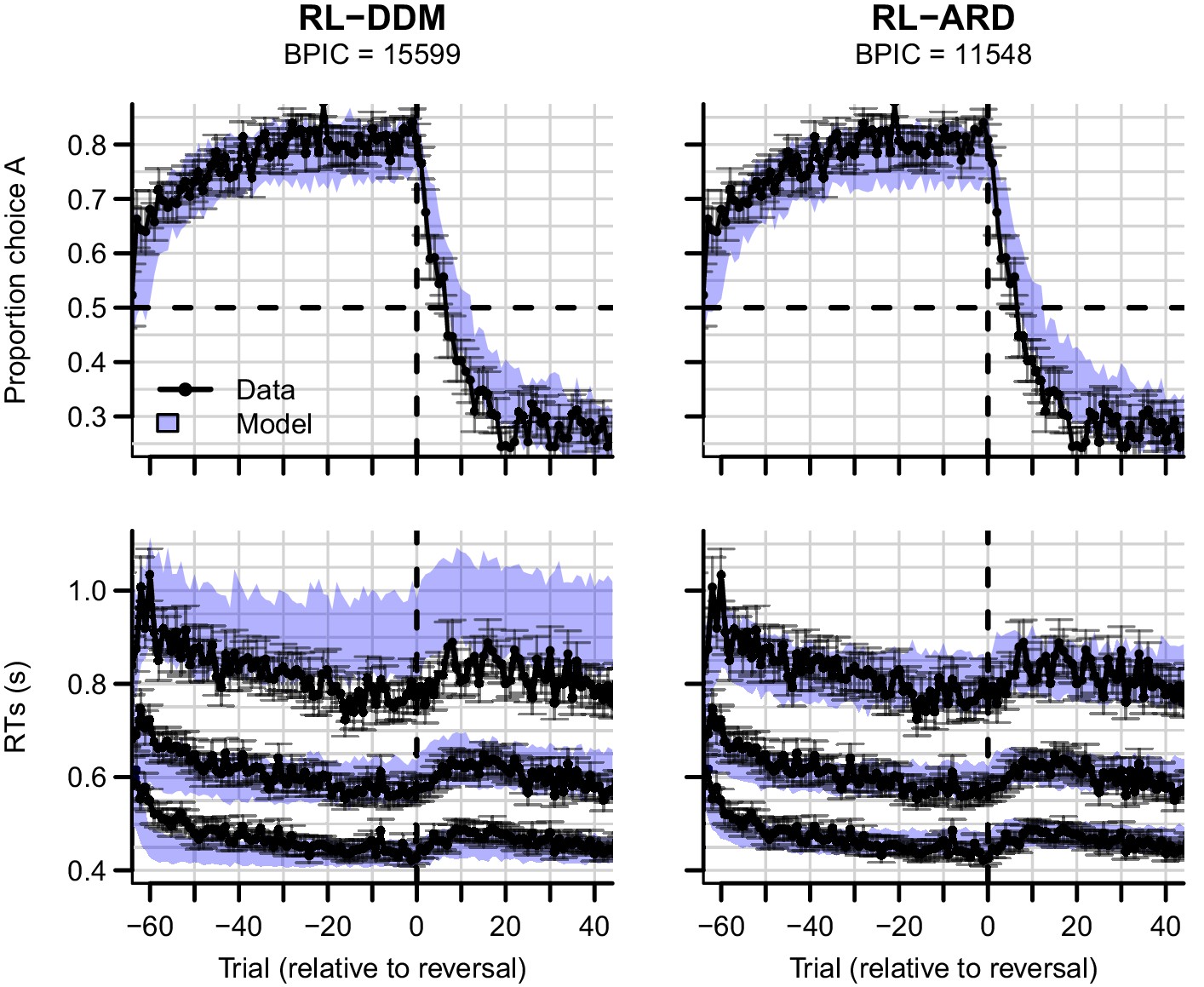
Experiment three data (black) and posterior predictive distributions (blue) for the RL-DDM (left) and RL-ARD (right).
Top row: choice proportions over trials, with choice option A defined as the high-probability choice before the reversal in reward contingencies. Bottom row: 10th, 50th, and 90th RT percentiles. The data are ordered relative to the trial at which the reversal first occurred (trial 0, with negative trial numbers indicated trials prior to the reversal). Shaded areas correspond to the 95% credible interval of the posterior predictive distributions.
Figure 7—figure supplement 1
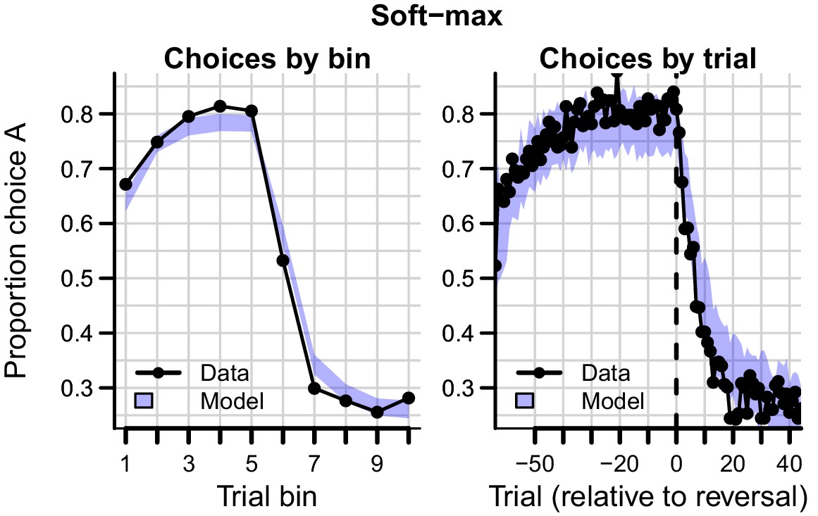
Data (black) of experiment 3 and posterior predictive of a standard soft-max learning model (blue).
As priors, we used truncated at 0 for the hypermean and for the hyperSD. Left panel depicts choice proportions for option over trial bins, where choice A is defined as the high-probability reward choice prior to the reversal. Right column depicts choice proportion over trials, aligned to the trial at which the reversal occurred (trial 0). Shaded areas correspond to the 95% credible interval of the posterior predictive distributions.
Figure 7—figure supplement 2
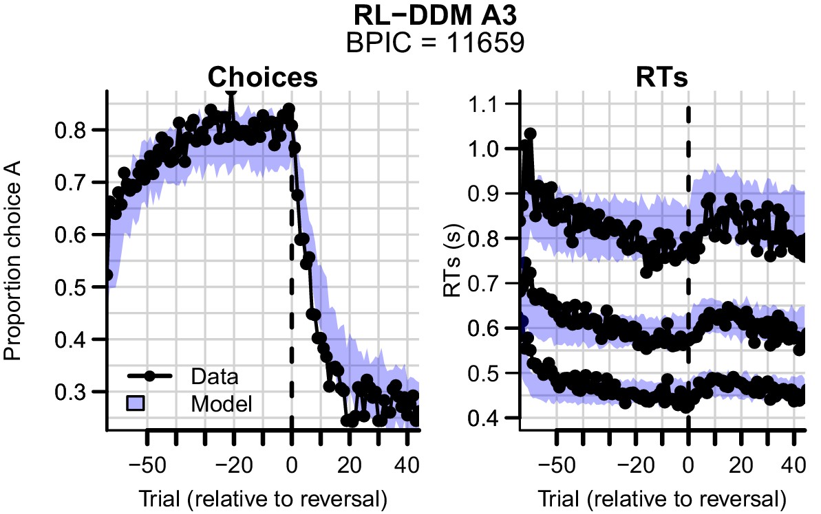
Data (black) of experiment 3 and posterior predictive distribution (blue) of the RL-DDM A3 (with between-trial variabilities in drift rates, start points, and non-decision times).
The summed BPIC was 11659. This is better compared to the RL-DDM () but did not outperform the RL-ARD ( in favor of the RL-ARD).
Figure 7—figure supplement 3
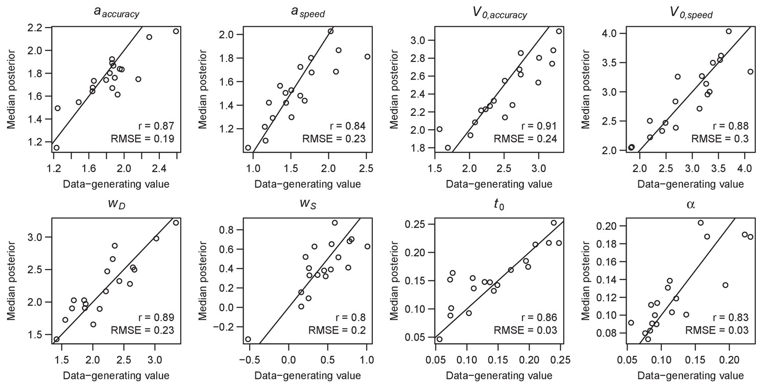
Parameter recovery of the RL-ARD model, using the experimental paradigm of experiment 3.
Parameter recovery was done by first fitting the RL-ARD model to the empirical data, and then simulating the exact same experimental paradigm (49 subjects, 2 difficulty conditions, 512 trials, including reversals) using the median parameter estimates obtained from the model fit. Subsequently, the RL-ARD was fit to the simulated data. The median posterior estimates (y-axis) are plotted against the data-generating values (x-axis). Pearson’s correlation coefficient r and the root mean square error (RMSE) are shown in each panel. Diagonal lines indicate the identity x = y.
Figure 7—figure supplement 4
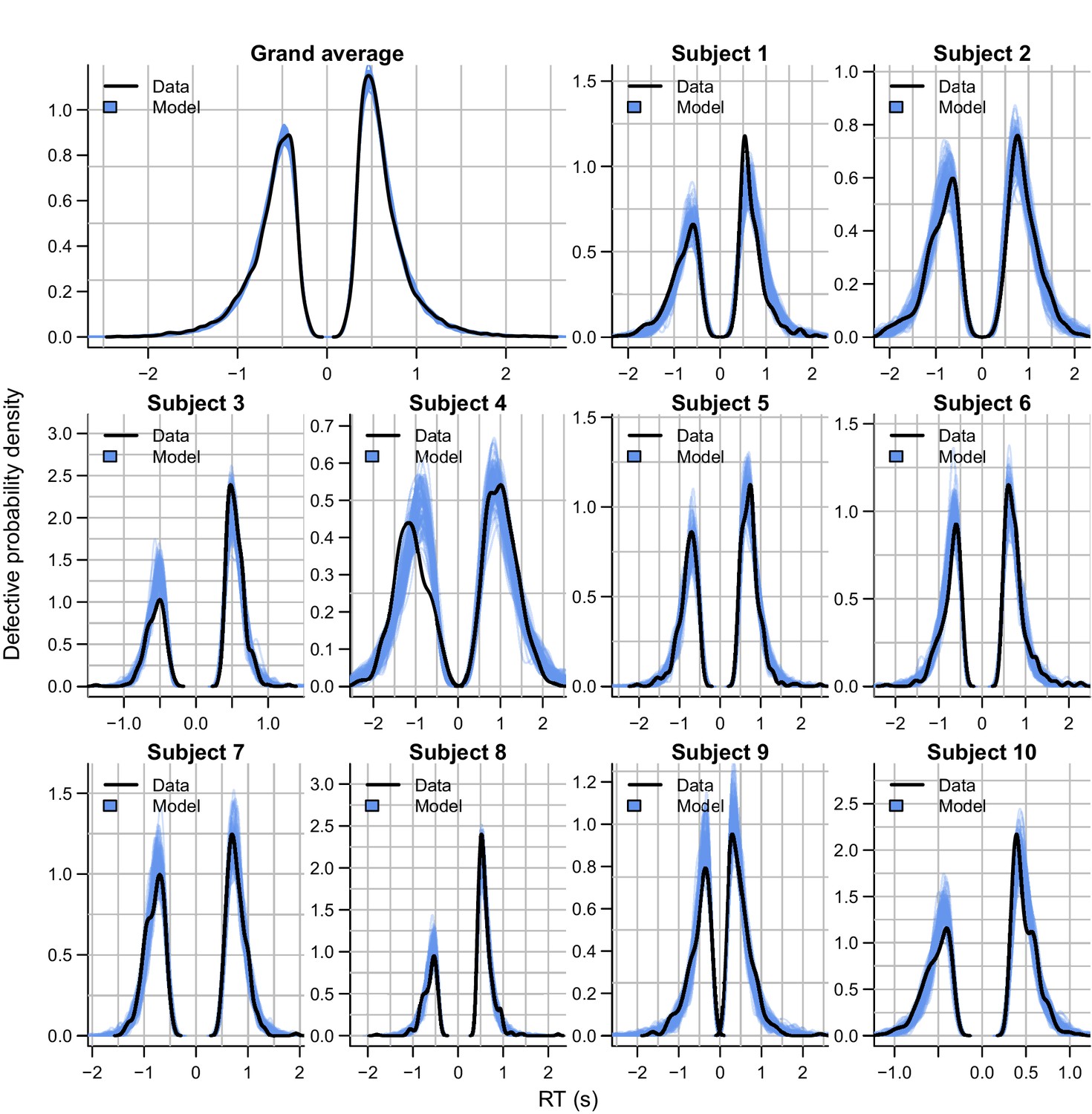
Empirical (black) and posterior predictive (blue) defective probability densities of the RT distributions of experiment 3, estimated using kernel density approximation.
Negative RTs correspond to choices for the option that was correct after the reversal. Blue lines represent 100 posterior predictive RT distributions from the RL-ARD model. The grand average is the RT distribution across all trials and subjects, subject-wise RT distributions are across all trials per subject for the first 10 subjects, for which the quality of fit was representative for the entire dataset.
Figure 7—figure supplement 5
Experiment three data (black) and posterior predictive distributions (blue) for the RL-DDM (left) and RL-ARD (right).
Top row: choice proportions over trials, with choice option A defined as the high-probability choice before the reversal in reward contingencies. Bottom row: 10th, 50th, and 90th RT percentiles. The data are ordered relative to the trial at which the reversal first occurred (trial 0, with negative trial numbers indicated trials prior to the reversal). Shaded areas correspond to the 95% credible interval of the posterior predictive distributions. Error bars depict standard errors.
Figure 8
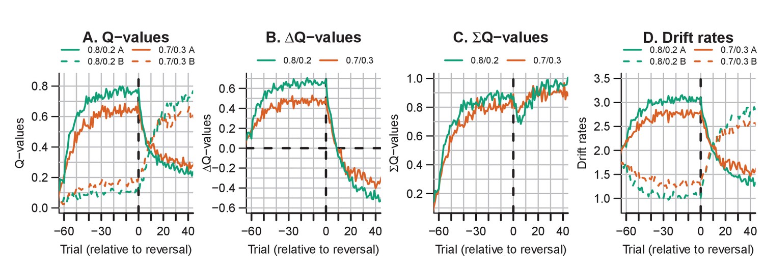
The evolution of Q-values and their effect on drift rates in the RL-ARD in experiment 3, aggregated across participants.
Left panel depicts raw Q-values, separate for each difficulty condition (colors). The second and third panel depict the Q-value differences and the Q-value sums over time. The drift rates (right panel) are a weighted sum of the Q-value differences and Q-value sums, plus an intercept. Choice A (solid lines) refers to the option that had the high probability of reward during the acquisition phase, and choice B (dashed lines) to the option that had the high probability of reward after the reversal.
Figure 9
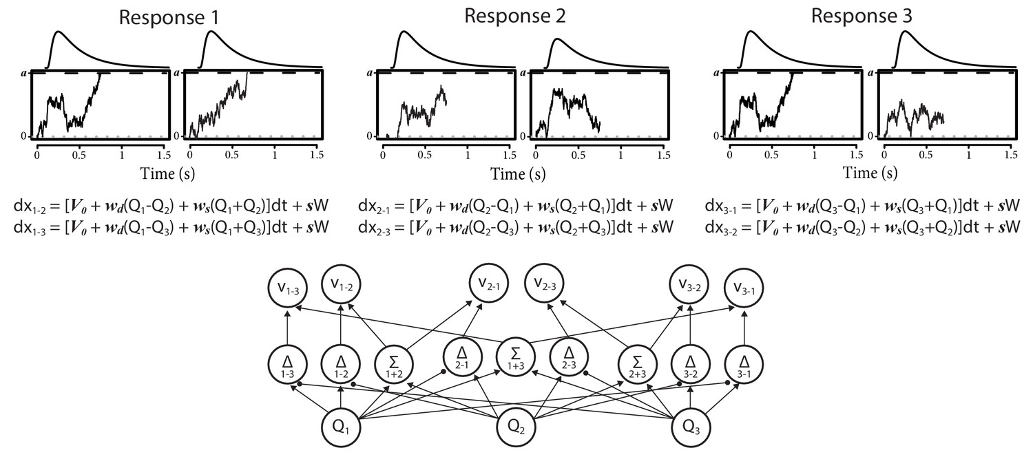
Architecture of the three-alternative RL-ARD.
In three-choice settings, there are three Q-values. The multi-alternative RL-ARD has one accumulator per directional pairwise difference, hence there are six accumulators. The bottom graph visualizes the connections between Q-values and drift rates ( is left out to improve readability). The equations formalize the within-trial dynamics of each accumulator. Top panels illustrate one example trial, in which both accumulators corresponding to response option 1 reached their thresholds. In this example trial, the model chose option 1, with the RT determined by the slowest of the winning accumulators (here, the leftmost accumulator). Decision-related parameters are all identical across the six accumulators.
Figure 10
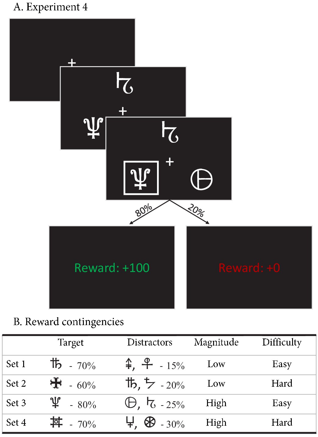
Experimental paradigm of experiment 4.
(A) Example trial of experiment 4. Each trial started with a fixation cross, followed by the stimulus (three choice options; until the subject made a choice, up to 3 s), a brief highlight of the choice, and the choice’s reward was shown. (B) Reward contingencies for the target stimulus and two distractors per condition. Percentages indicate the probability of receiving +100 points (+0 otherwise). Presented symbols are examples, the actual symbols differed per block and participant (counterbalanced to prevent potential item effects from confounding the learning process).
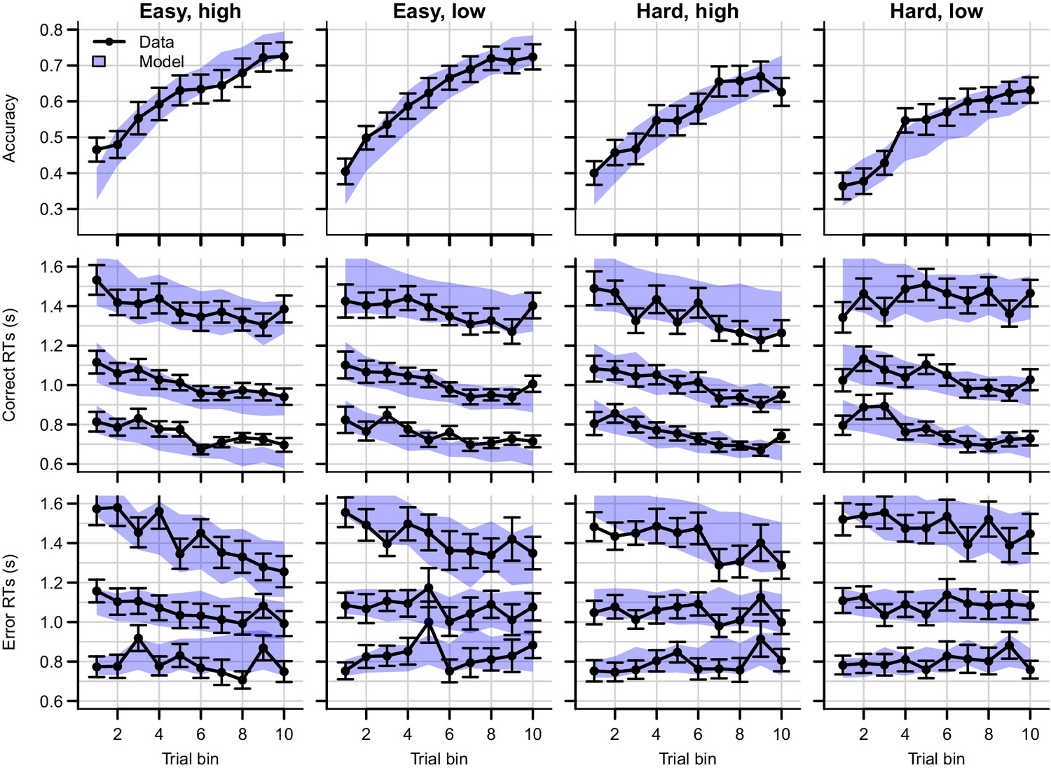
Figure 11 with 3 supplements
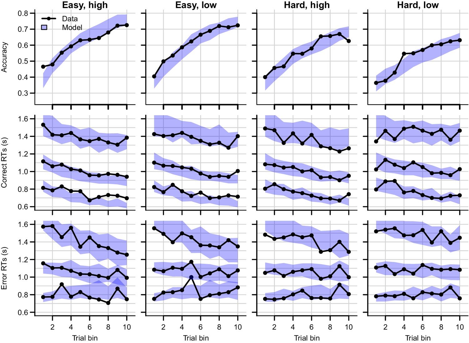
Data (black) and posterior predictive distribution of the RL-ARD (blue), separately for each difficulty condition.
Column titles indicate the magnitude and difficulty condition. Top row depicts accuracy over trial bins. Middle and bottom rows show 10th, 50th, and 90th RT percentiles for the correct (middle row) and error (bottom row) response over trial bins. The error responses are collapsed across distractors. Shaded areas correspond to the 95% credible interval of the posterior predictive distributions. All data and fits are collapsed across participants.
Figure 11—figure supplement 1
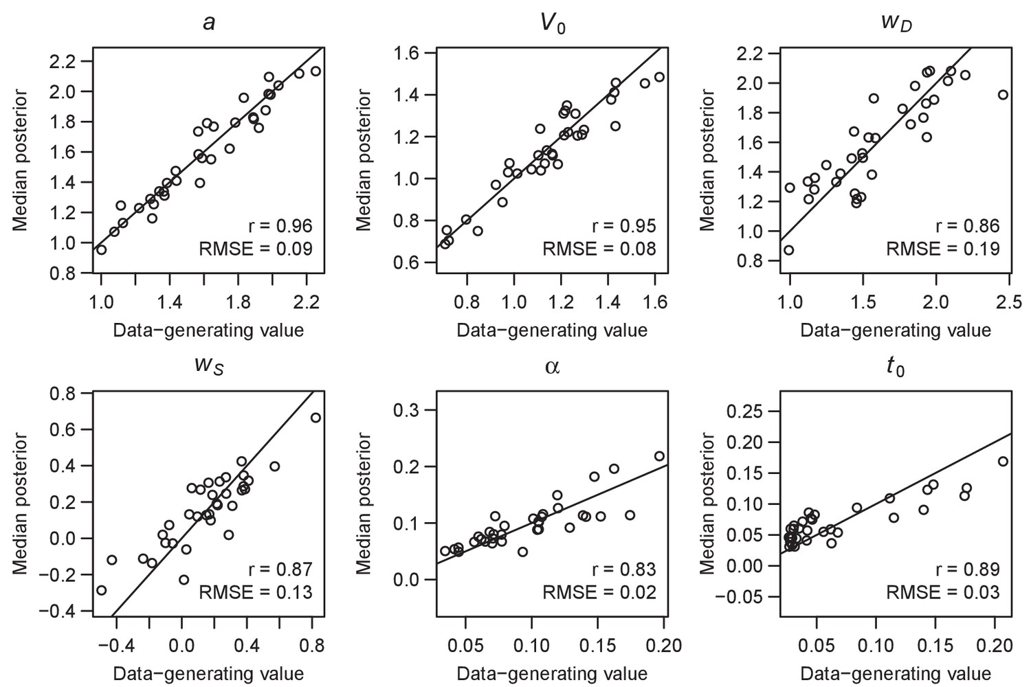
Parameter recovery of the multi-alterative Win-All RL-ARD model, using the experimental paradigm of experiment 4.
Parameter recovery was done by first fitting the RL-ARD model to the empirical data, and then simulating the exact same experimental paradigm (34 subjects, 4 conditions, 432 trials) using the median parameter estimates obtained from the model fit. Subsequently, the RL-ARD was fit to the simulated data. The median posterior estimates (y-axis) are plotted against the data-generating values (x-axis). Pearson’s correlation coefficient r and the root mean square error (RMSE) are shown in each panel. Diagonal lines indicate the identity x = y.
Figure 11—figure supplement 2
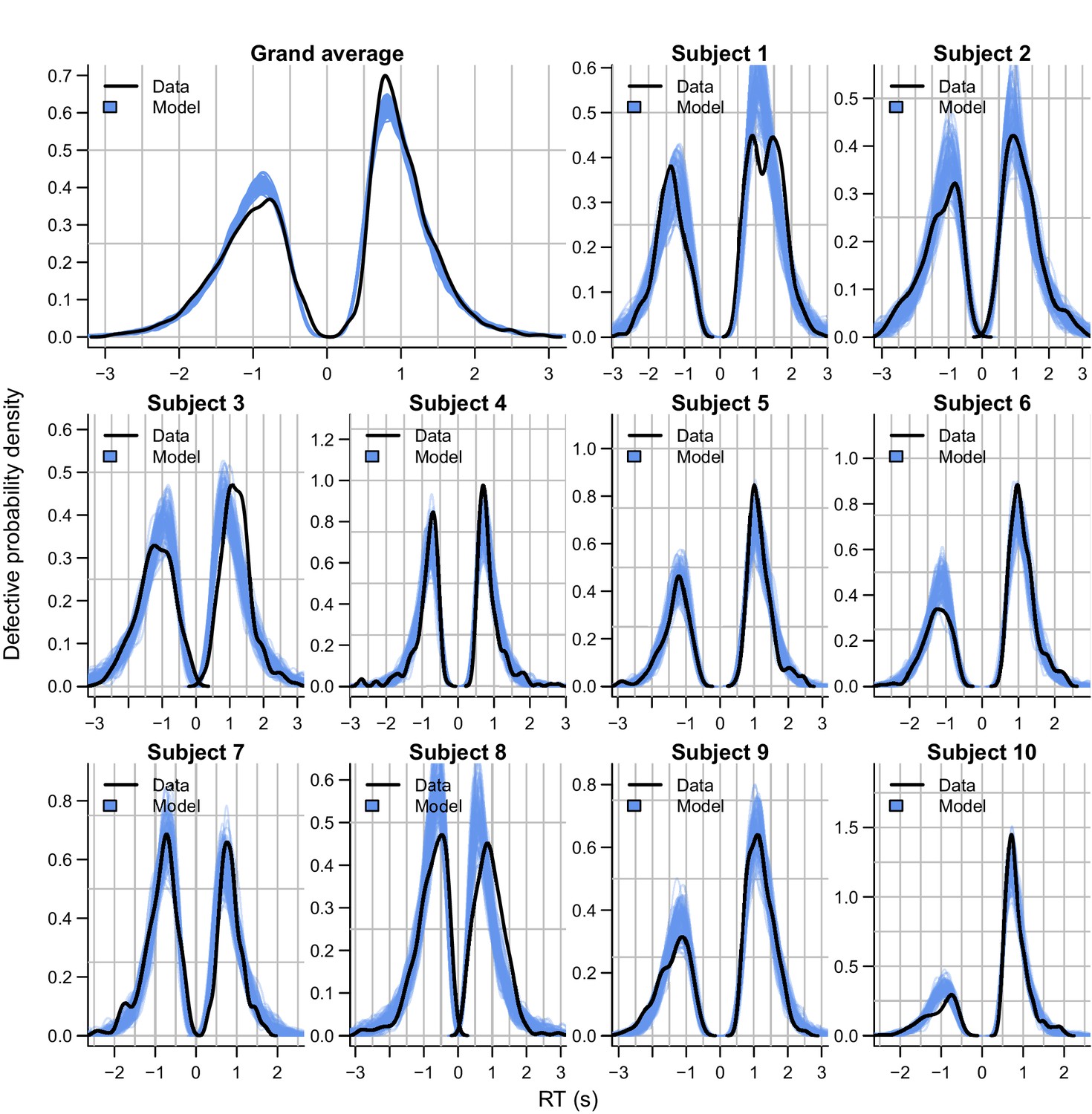
Empirical (black) and posterior predictive (blue) defective probability densities of the RT distributions of experiment 4, estimated using kernel density approximation.
Negative RTs correspond to error choices, collapsed across the two distractor choice options. Blue lines represent 100 posterior predictive RT distributions from the RL-ARD model. The grand average is the RT distribution across all trials and subjects, subject-wise RT distributions are across all trials per subject for the first 10 subjects, for which the quality of fit was representative for the entire dataset.
Figure 11—figure supplement 3
Data (black) and posterior predictive distribution of the RL-ARD (blue), separately for each difficulty condition of experiment 4.
Column titles indicate the magnitude and difficulty condition. Top row depicts accuracy over trial bins. Middle and bottom rows show 10th, 50th, and 90th RT percentiles for the correct (middle row) and error (bottom row) response over trial bins. The error responses are collapsed across distractors. Shaded areas correspond to the 95% credible interval of the posterior predictive distributions. All data and fits are collapsed across participants. Error bars depict standard errors.
Figure 12
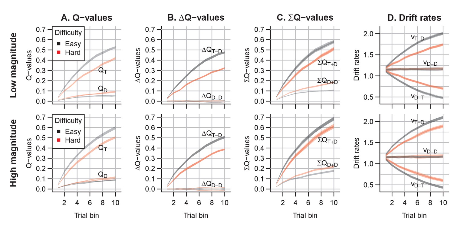
Q-value evolution in experiment 4.
Top row corresponds to the low magnitude condition, bottom to the high magnitude condition. Colors indicate choice difficulty. (A) Q-values for target () and distractor stimuli (). (B) Difference in Q-values, for target – distractor () and between the two distractors (). The Q-value difference is omitted from the graph to aid readability (but ). (C) Sum of Q-values. (D) Resulting drift rates for target response accumulators (), and accumulators for the distractor choice options (. Note that within each condition, there is a single Q-value trace per choice option, but since there are two distractors, there are two overlapping traces for , , and for all drift rates.
Tables
Table 1
Posterior parameter estimates (across-subject mean and SD of the median of the posterior distributions) for all models and experiments.
For models including , the non-decision time is assumed to be uniformly distributed with bounds .
| Experiment 1 | |||||||||
|---|---|---|---|---|---|---|---|---|---|
| RL-DDM | BPIC | ||||||||
| 0.14 (0.11) | 1.48 (0.19) | 0.30 (0.06) | 3.21 (1.11) | 7673 | |||||
| RL-RD | |||||||||
| 0.12 (0.08) | 2.16 (0.27) | 0.10 (0.04) | 1.92 (0.42) | 3.09 (1.32) | 5613 | ||||
| RL-lARD | |||||||||
| 0.13 (0.12) | 2.05 (0.24) | 0.12 (0.05) | 2.48 (0.43) | 2.36 (0.95) | 4849 | ||||
| RL-ARD | |||||||||
| 0.13 (0.11) | 2.14 (0.26) | 0.11 (0.04) | 2.46 (0.59) | 2.25 (0.78) | 0.36 (0.79) | 4577 | |||
| RL-DDM A1 | |||||||||
| 0.14 (0.12) | 1.49 (0.20) | 0.30 (0.06) | 3.01 (0.66) | 2.81 (0.72) | 7717 | ||||
| RL-DDM A2 | |||||||||
| 0.14 (0.11) | 1.48 (0.19) | 0.30 (0.06) | 3.21 (1.12) | 1.79e−3 (0.4e−3) | 1.8e−3 (0.4e-3) | 7637 | |||
| RL-DDM A3 | |||||||||
| 0.13 (0.12) | 1.13 (0.19) | 0.27 (0.06) | 5.31 (2.04) | 0.00 (0.00) | 0.31 (0.13) | 0.37 (0.13) | 4844 | ||
| RL-DDM A4 | |||||||||
| 0.13 (0.12) | 1.15 (0.17) | 0.27 (0.06) | 2.02 (0) | 5.16 (1.18) | 0.55 (0.24) | 1.57e−3 (0) | 0.36 (0.13) | 4884 | |
| RL-ALBA | A | ||||||||
| 0.13 (0.11) | 3.53 (0.53) | 0.03 (0.00) | 3.03 (0.57) | 2.03 (0.59) | 0.33 (0.78) | 1.73 (0.43) | 4836 | ||
| Experiment 2 | |||||||||
| RL-DDM 1 | / | ||||||||
| 0.13 (0.06) | 1.11 (0.18)/1.42 (0.23) | 0.26 (0.06) | 3.28 (0.66) | 979 | |||||
| RL-DDM 2 | / | ||||||||
| 0.13 (0.05) | 3.01 (0.63) | 0.26 (0.06) | 3.46 (0.79)/3.01 (0.63) | 1518 | |||||
| RL-DDM 3 | / | / | |||||||
| 0.13 (0.06) | 1.10 (0.18)/1.44 (0.23) | 0.26 (0.06) | 3.11 (0.68)/3.48 (0.72) | 999 | |||||
| RL-ARD 1 | |||||||||
| 0.12 (0.05) | 1.45 (0.35)/1.82 (0.35) | 0.15 (0.07) | 2.59 (0.50) | 2.24 (0.53) | 0.47 (0.34) | −1044 | |||
| RL-ARD 2 | |||||||||
| 0.12 (0.05) | 1.83 (0.36) | 0.12 (0.07) | 2.52 (0.53) | 1.83 (0.56) | 0.32 (0.26) | 1.31 (0.20) | −827 | ||
| RL-ARD 3 | / | ||||||||
| 0.12 (0.05) | 1.83 (0.35) | 0.12 (0.07) | 3.37 (0.84)/3.37 (0.54) | 2.11 (0.52) | 0.39 (0.30) | −934 | |||
| RL-ARD 4 | |||||||||
| 0.12 (0.05) | 1.04 (0.14)/1.82 (0.35) | 0.15 (0.07) | 2.59 (0.52) | 2.21 (0.51) | 0.44 (0.38) | 1.04 (0.14) | −1055 | ||
| RL-ARD 5 | / | / | |||||||
| 0.12 (0.05) | 1.59 (0.40)/1.83 (0.32) | 0.14 (0.06) | 2.92 (0.65)/2.52 (0.50) | 2.21 (0.50) | 0.43 (0.33) | −1071 | |||
| RL-ARD 6 | / | ||||||||
| 0.12 (0.05) | 1.86 (0.35) | 0.12 (0.07) | 4.13 (0.98)/2.40 (0.54) | 2.28 (0.53) | 0.44 (0.33) | 0.84 (0.03) | −897 | ||
| RL-ARD 7 | / | / | |||||||
| 0.12 (0.05) | 1.61 (0.40)/1.87 (0.32) | 0.14 (0.06) | 3.66 (0.74)/2.52 (0.50) | 2.41 (0.53) | 0.48 (0.38) | 0.82 (0.08) | −1060 | ||
| RL-DDM A3 1 | / | ||||||||
| 0.12 (0.05) | 0.81 (0.16)/1.14 (0.17) | 0.23 (0.06) | 4.46 (0.79) | 0.10 (0.01) | 0.18 (0.05) | 0.26 (0.09) | −862 | ||
| RL-DDM A3 2 | / | ||||||||
| 0.12 (0.05) | 1.03 (0.14) | 0.24 (0.06) | 18.4 (23.34)/4.44 (0.84) | 0.26 (0.07) | 0.61 (0.50) | 0.28 (0.10) | −325 | ||
| RL-DDM A3 3 | / | / | |||||||
| 0.12 (0.05) | 0.81 (0.16)/1.14 (0.17) | 0.23 (0.06) | 4.45 (0.83)/4.45 (0.83) | 0.07 (0.00) | 0.17 (0.04) | 0.26 (0.09) | −849 | ||
| Experiment 3 | |||||||||
| Soft-max | |||||||||
| 0.40 (0.14) | 2.82 (1.1) | 23,727 | |||||||
| RL-DDM | |||||||||
| 0.38 (0.14) | 1.37 (0.24) | 0.24 (0.07) | 15,599 | ||||||
| RL-ARD | |||||||||
| 0.35 (0.15) | 1.48 (0.34) | 0.13 (0.08) | 1.86 (0.51) | 1.52 (0.63) | 0.23 (0.25) | 11,548 | |||
| RL-DDM A3 | |||||||||
| 0.38 (0.14) | 1.15 (0.22) | 0.22 (0.07) | 2.72 (1.16) | 0.21 (0.09) | 0.28 (0.15) | 0.27 (0.17) | 11,659 | ||
| Experiment 4 | |||||||||
| RL-ARD (Win-All) | |||||||||
| 0.10 (0.04) | 1.6 (0.33) | 0.07 (0.05) | 1.14 (0.22) | 1.6 (0.36) | 0.15 (0.26) | 36,512 | |||
Additional files
Download links
A two-part list of links to download the article, or parts of the article, in various formats.
Downloads (link to download the article as PDF)
Open citations (links to open the citations from this article in various online reference manager services)
Cite this article (links to download the citations from this article in formats compatible with various reference manager tools)
A new model of decision processing in instrumental learning tasks
eLife 10:e63055.
https://doi.org/10.7554/eLife.63055


