Sexual dimorphism in trait variability and its eco-evolutionary and statistical implications
- Evolution & Ecology Research Center, School of Biological, Earth, and Environmental Sciences, University of New South Wales, Australia
- Liverpool John Moores University, School of Biological and Environmental Sciences, United Kingdom
- European Bioinformatics Institute (EMBL-EBI), European Molecular Biology Laboratory, Wellcome Trust Genome Campus, United Kingdom
- University of Sydney, Charles Perkins Centre, School of Life and Environmental Sciences, School of Mathematics and Statistics, Australia
- Division of Ecology and Evolution, Research School of Biology, Australian National University, Australia
Figures
Figure 1 with 1 supplement
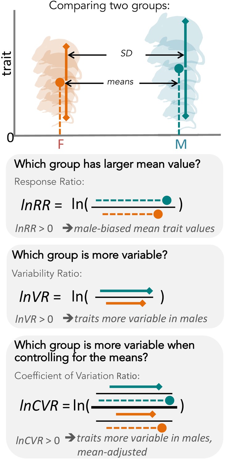
Overview of meta-analytic methods used to detect differences in means and variances in any given trait (e.g. body size in mice).
The orange shading represents females (F), turquoise shading stands for males (M). The solid circle represents a mean trait value within the respective group. Solid lines represent standard deviation, with upper and lower bounds indicated by diamond shapes. Below, we present three types of effect sizes that can be used for comparing two groups, along with the respective formulas and interpretations. Compared to lnVR (the ratio of SD), lnCVR (the ratio of CV or relative variance) provides a more general measure of the difference in variability between two groups (mean-adjusted variability ratio).
Figure 1—figure supplement 1
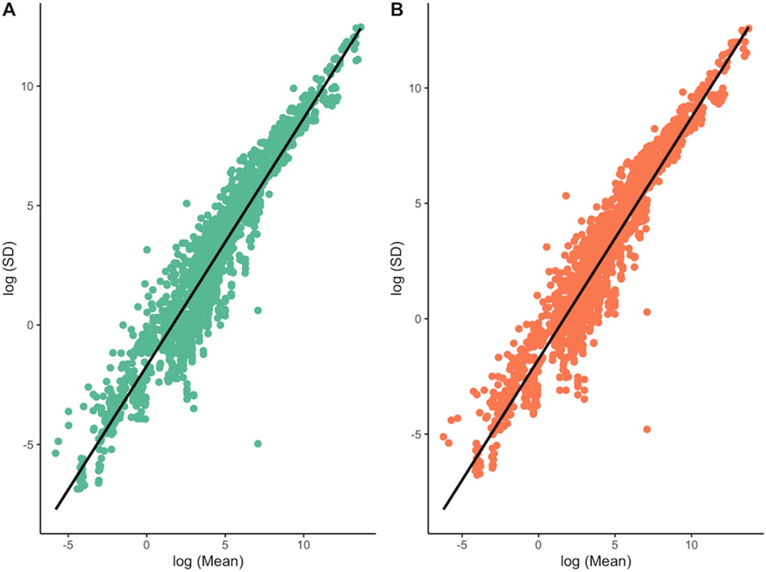
Mean-variance relationships (log(Mean) vs log(SD, standard deviation)) across all traits for males (A) and females (B).
Figure 2
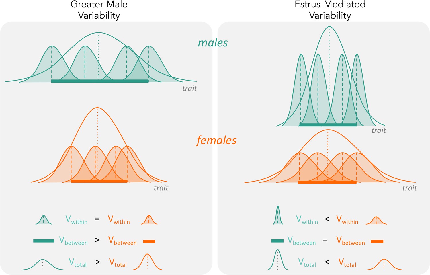
The two hypotheses (‘greater male variability’ versus ‘estrus-mediated variability’) have different predictions on how variabilities influence total observed phenotypic variance (Vtotal in the figure).
For greater male variability, the within-subject (or within-trait) variation Vwithin could be potentially negligible or is equal in males and females. This is illustrated as the shaded distributions around each individual mean (dashed vertical lines), which are of equal area for the males (turquoise) and females (orange). The greater value of Vtotal is driven by wider distribution of mean trait values in males compared to females (i.e. Vbetween, represented by a thick horizontal bar). The estrus-mediated variability hypothesis, in contrast, assumes that within-subject [or within-trait] variability is much higher in females than in males (broader orange-shaded trait distributions than turquoise distributions), while the variability of the means between individuals stays the same (thick horizontal bars).
Figure 3

Workflow of data processing and meta-analysis.
Figure 4 with 2 supplements

Sex bias in trait groups.
Panel (A) shows the numbers of traits that are either male-biased (turquoise) or female-biased (orange) across functional groups. The x-axes in Panel A represents the overall percentages of traits with a given direction of sex bias: orange shading when meta-analytic mean < 0 (female-biased), turquoise shading when meta-analytic mean > 0 (male-biased). White numbers inside the turquoise bars represent numbers of traits that show male bias within a given group of traits, numbers inside the orange bars represent the number of female-biased traits. Panel (B) shows effect sizes and 95% CI from separate meta-analysis for each functional group (Figure 3H). Traits that are male-biased in Panel B are shifted towards the righthand side of the zero-midline (near the turquoise male symbol), whereas female-biased traits are shifted towards the left (near the orange female symbol).
-
Figure 4—source data 1
Numbers of sex-biased traits.
- https://cdn.elifesciences.org/articles/63170/elife-63170-fig4-data1-v2.csv.zip
-
Figure 4—source data 2
Effect sizes of sex bias in functional groups.
- https://cdn.elifesciences.org/articles/63170/elife-63170-fig4-data2-v2.csv.zip
Figure 4—figure supplement 1
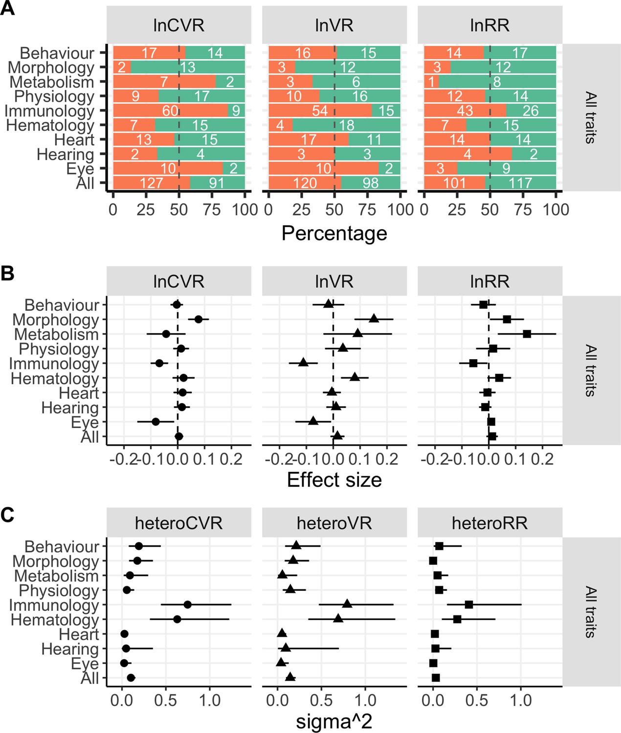
Percentages and numbers of either male (turqoise bars) or female (orange bars) biased traits (Panel A) across functional groups, this time for lnCVR (left hand side), lnVR (middle) and lnRR (right hand side).
Panel B shows effect sizes from separate meta-analysis for each functional group, and Panel C contains results of heterogeneity analyses. All three panels represent results evaluated across all traits.
Figure 4—figure supplement 2
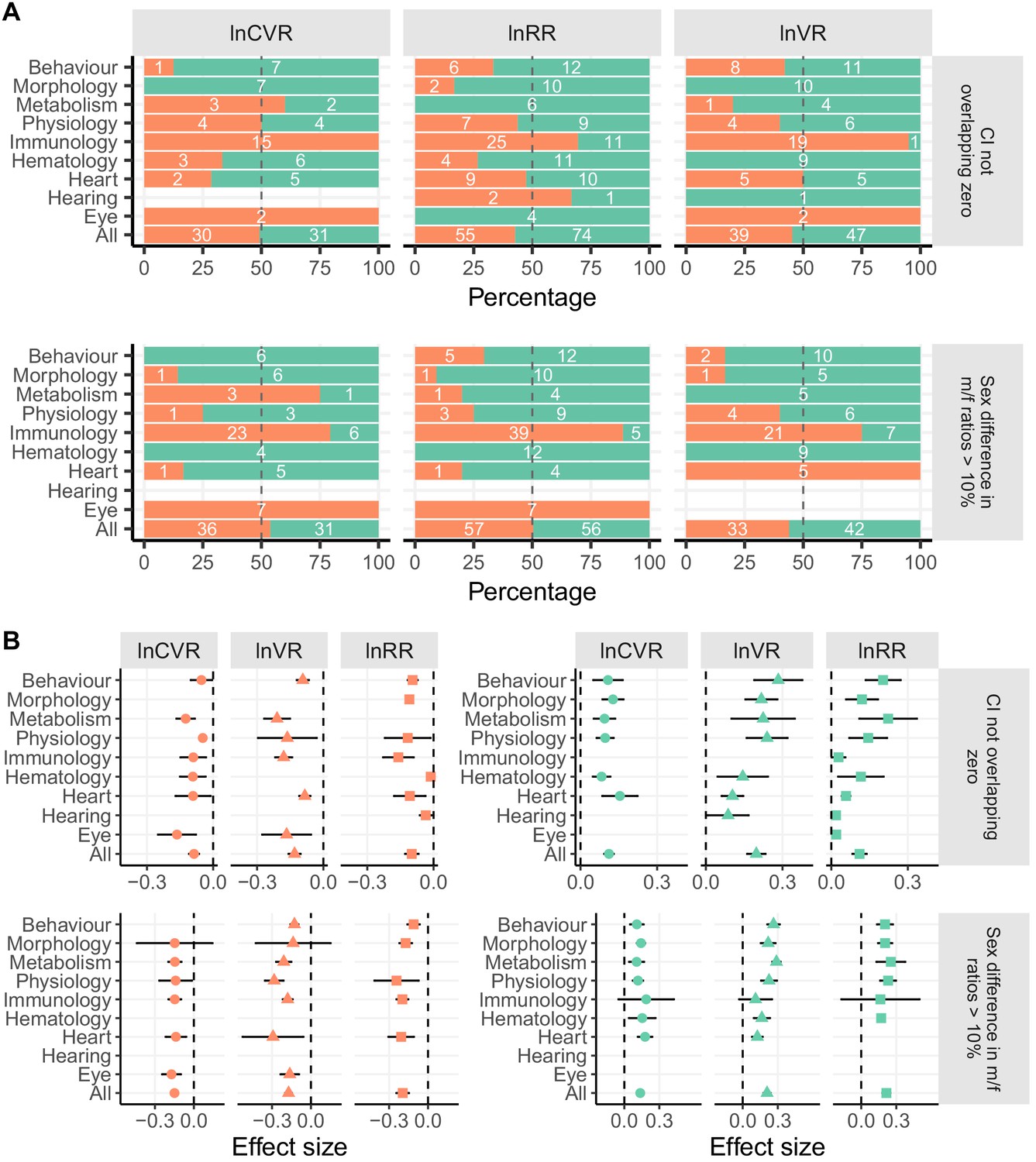
Sex bias in trait groups for lnCVR, lnVR and lnRR.
(A) Percentages and numbers of affected traits, for variance (lnCVR and lnVR) and means (lnRR), where there is a significant difference between the sexes (i.e. CI not overlapping zero), and where the sex bias is greater than 10% difference (regardless of significance). Panel B depicts results for the effect size magnitudes in those traits that differ between the sexes (second-order meta-analysis). Triangles represent sex bias in means (response ratio) and black circles differences in the coefficient of variation ratio (mean-adjusted variability). The orange bars represent trait groups with a female bias, turqouise bars male-biased traits.
Figure 5
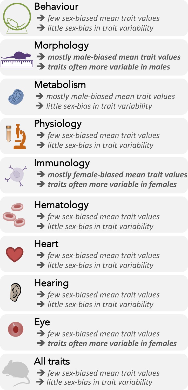
Summary of sex differences in the mean trait values (lnRR) and variances (lnCVR) across nine functional trait groups, and overall.
Additional files
-
Source code 1
This markdown file contains all steps from processing the raw data file through to meta-analyses to Figure and table generation.
The knitted html version can be viewed at https://rpubs.com/SusZaj/ESF.
- https://cdn.elifesciences.org/articles/63170/elife-63170-code1-v2.zip
-
Supplementary file 1
Supplementary tables.
Table 1. Summary of the available numbers of male and female mice from each strain and originating institution Table 2. Trait categories (parameter_group) and the number of correlated traits within these categories. Traits were meta-analysed using robumeta Table 3. We use this corrected (for correlated traits) results table, which contains each of the meta-analytic means for all effect sizes of interest, for further analyses. We further use this table as part of the Shiny App, which is able to provide the percentage differences between males and females for mean, variance and coefficient of variance (continued below) (Table 4). Summary of overall meta-analyses on the functional trait group level (GroupingTerm). Results for lnCVR, lnVR and lnRR and their respective upper and lower 95 percent CI’s, standard error and I2 values are provided. Values truncated at five decimal places for readability. Table 5. Provides an overview of meta-analysis results performed on traits that were significantly biased towards either sex. This table summarizes findings for both sexes and the respective functional trait groups. Values truncated at five decimal places for readability. Table 6. Summarizes our findings on heterogeneity due to institutions and mouse strains. These results are based on meta-analyses on sigma2 and errors for mouse strains and centres (Institutions), following the identical workflow from above. Values truncated at five decimal places for readability.
- https://cdn.elifesciences.org/articles/63170/elife-63170-supp1-v2.docx
-
Transparent reporting form
- https://cdn.elifesciences.org/articles/63170/elife-63170-transrepform-v2.docx
Download links
A two-part list of links to download the article, or parts of the article, in various formats.
Downloads (link to download the article as PDF)
Open citations (links to open the citations from this article in various online reference manager services)
Cite this article (links to download the citations from this article in formats compatible with various reference manager tools)
Sexual dimorphism in trait variability and its eco-evolutionary and statistical implications
eLife 9:e63170.
https://doi.org/10.7554/eLife.63170


