Sexual dimorphism in trait variability and its eco-evolutionary and statistical implications
Abstract
Biomedical and clinical sciences are experiencing a renewed interest in the fact that males and females differ in many anatomic, physiological, and behavioural traits. Sex differences in trait variability, however, are yet to receive similar recognition. In medical science, mammalian females are assumed to have higher trait variability due to estrous cycles (the ‘estrus-mediated variability hypothesis’); historically in biomedical research, females have been excluded for this reason. Contrastingly, evolutionary theory and associated data support the ‘greater male variability hypothesis’. Here, we test these competing hypotheses in 218 traits measured in >26,900 mice, using meta-analysis methods. Neither hypothesis could universally explain patterns in trait variability. Sex bias in variability was trait-dependent. While greater male variability was found in morphological traits, females were much more variable in immunological traits. Sex-specific variability has eco-evolutionary ramifications, including sex-dependent responses to climate change, as well as statistical implications including power analysis considering sex difference in variance.
eLife digest
Males and females differ in appearance, physiology and behavior. But we do not fully understand the health and evolutionary consequences of these differences. One reason for this is that, until recently, females were often excluded from medical studies. This made it difficult to know if a treatment would perform as well in females as males. To correct this, organizations that fund research now require scientists to include both sexes in studies. This has led to some questions about how to account for sex differences in studies.
One reason females have historically been excluded from medical studies is that some scientists assumed that they would have more variable responses to a particular treatment based on their estrous cycles. Other scientists, however, believe that males of a given species might be more variable because of the evolutionary pressures they face in competing for mates. Better understanding how males and females vary would help scientists better design studies to ensure they provide accurate answers.
Now, Zajitschek et al. debunk both the idea that males are more variable and the idea that females are more variable. To do this, Zajitschek et al. analyzed differences in 218 traits, like body size or certain behaviors, among nearly 27,000 male and female mice. This showed that neither male mice nor female mice were universally more different from other mice of their sex across all features. Instead, sex differences in how much variation existed in male or female mice depended on the individual trait. For example, males varied more in physical features like size, while females showed more differences in their immune systems.
The results suggest it is particularly important to consider sex-specific variability in both medical and other types of studies. To help other researchers better design experiments to factor in such variability, Zajitschek et al. created an interactive tool that will allow scientists to look at sex-based differences in individual features among male or female mice.
Introduction
Sex differences arise because selection acts on the two sexes differently, especially on traits associated with mating and reproduction (Darwin, 1871). Therefore, sex differences are widespread, a fact which is unsurprising to any evolutionary biologist. However, scientists in many (bio-)medical fields have not necessarily regarded sex as a biological factor of intrinsic interest (Clayton, 2016; Flanagan, 2014; Karp et al., 2017; Klein et al., 2015; Prendergast et al., 2014; Shansky and Woolley, 2016). Therefore, many (bio-)medical studies have only been conducted with male subjects. Consequently, our knowledge is biased. For example, we know far more about drug efficacy in male compared to female subjects, contributing to a poor understanding of how the sexes respond differently to medical interventions (Nowogrodzki, 2017). This gap in knowledge is predicted to lead to overmedication and adverse drug reactions in women (Zucker and Prendergast, 2020). Only recently have (bio-)medical scientists started considering sex differences in their research (Dorris et al., 2015; Ingvorsen et al., 2017; Robinson et al., 2017; Smarr et al., 2017; Ahmad et al., 2017; Foltin and Evans, 2018; Thompson et al., 2018). Indeed, the National Institutes of Health (NIH) have now implemented new guidelines for animal and human research study designs, requiring that sex be included as a biological variable (Clayton, 2016; Clayton and Collins, 2014; NIH, 2015a).
When comparing the sexes, biologists generally focus on mean differences in trait values, placing little or no emphasis on sex differences in trait variability (see Figure 1 for a diagram explaining differences in means and variances). Despite this, two hypotheses exist that explain why trait variability might be expected to differ between the sexes. Interestingly, these two hypotheses make opposing predictions.

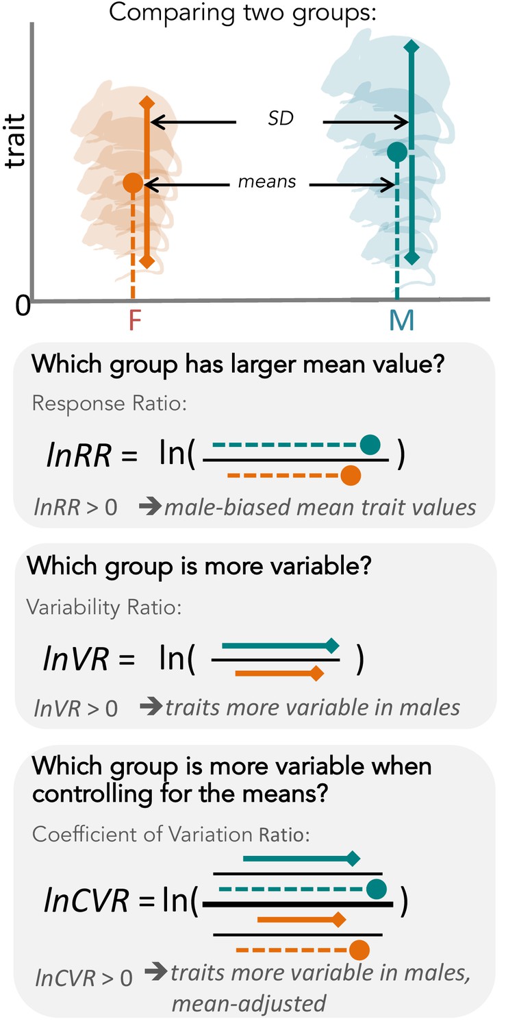
Overview of meta-analytic methods used to detect differences in means and variances in any given trait (e.g. body size in mice).
The orange shading represents females (F), turquoise shading stands for males (M). The solid circle represents a mean trait value within the respective group. Solid lines represent standard deviation, with upper and lower bounds indicated by diamond shapes. Below, we present three types of effect sizes that can be used for comparing two groups, along with the respective formulas and interpretations. Compared to lnVR (the ratio of SD), lnCVR (the ratio of CV or relative variance) provides a more general measure of the difference in variability between two groups (mean-adjusted variability ratio).
First, the ‘estrus-mediated variability hypothesis’ (Figure 2), which emerged in the (bio-)medical research field, assumes that the female estrous cycle (see e.g. Prendergast et al., 2014; Beery and Zucker, 2011) causes higher variability across traits in female subjects. A wide range of labile traits are presumed to co-vary with physiological changes that are induced by reproductive hormones. High variability is, therefore, expected to be particularly prominent when the stage of the estrous cycle is unknown and unaccounted for. This higher trait variability, resulting from females being at different stages of their estrous cycle, is the main reason for why female research subjects are often excluded from biomedical research trials, especially in the fields of neuroscience, physiology and pharmacology (NIH, 2015a). Female exclusion has traditionally been justified based on the grounds that including females in empirical research leads to a loss of statistical power, or that animals must be sampled across the estrous cycle for one to make valid conclusions, requiring more time and resources.

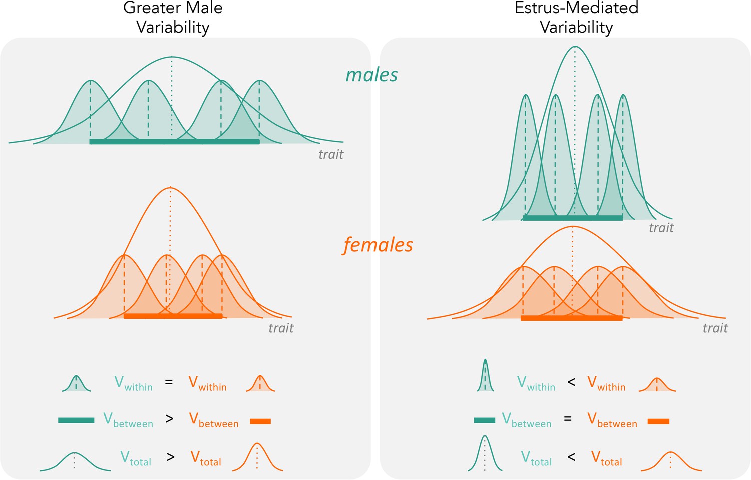
The two hypotheses (‘greater male variability’ versus ‘estrus-mediated variability’) have different predictions on how variabilities influence total observed phenotypic variance (Vtotal in the figure).
For greater male variability, the within-subject (or within-trait) variation Vwithin could be potentially negligible or is equal in males and females. This is illustrated as the shaded distributions around each individual mean (dashed vertical lines), which are of equal area for the males (turquoise) and females (orange). The greater value of Vtotal is driven by wider distribution of mean trait values in males compared to females (i.e. Vbetween, represented by a thick horizontal bar). The estrus-mediated variability hypothesis, in contrast, assumes that within-subject [or within-trait] variability is much higher in females than in males (broader orange-shaded trait distributions than turquoise distributions), while the variability of the means between individuals stays the same (thick horizontal bars).
Second, the ‘greater male variability hypothesis’ suggests males exhibit higher trait variability because of two different mechanisms. The first mechanism is based on males being the heterogametic sex in mammals. Mammalian females possess two X chromosomes, leading to an ‘averaging’ of trait expression across the genes on each chromosome. In contrast, males exhibit greater variance because expression of genes on a single X chromosome is likely to lead to more extreme trait values (Reinhold and Engqvist, 2013). The second mechanism is based on males being under stronger sexual selection (Pomiankowski and Moller, 1995; Cuervo and Møller, 1999; Cuervo and Møller, 2001). Empirical evidence supports higher variability of traits that are sexually selected, often harbouring high genetic variance and being condition-dependent, which makes sense as ‘condition’ as a trait is likely to be based on numerous loci (Rowe and Houle, 1996; Tomkins et al., 2004). Thus, higher genetic and, thus, phenotypic variance resulting from sexual selection is expected to characterise sexually selected traits. In mammals, it is likely that both mechanisms are operating concomitantly. So far, the ‘greater male variability hypothesis’ has gained some support in the evolutionary and psychological literature (Reinhold and Engqvist, 2013; Lehre et al., 2009).
Here, we conduct the first comprehensive test of the greater male variability and estrus-mediated variability hypotheses in mice (Figure 2; Reinhold and Engqvist, 2013; Johnson et al., 2008; Hedges and Nowell, 1995; Itoh and Arnold, 2015; Becker et al., 2016; Beery, 2018), examining sex differences in variance across 218 traits in 26,916 animals. To this end, we carry out a series of meta-analyses in two steps (Figure 3). First, we quantify the natural logarithm of the male to female coefficients of variation, CV, or relative variance (lnCVR) for each cohort (population) of mice, for different traits, along with the variability ratio of male to female standard deviations, SD, on the log scale (lnVR, following Nakagawa et al., 2015, see Figure 1). Then, we analyse these effect sizes to quantify sex bias in variance for each trait using meta-analytic methods. To better understand our results, and match them to previously reported sex differences in trait means (Karp et al., 2017), we also quantify and analyse the log response ratio (lnRR). Next, we statistically amalgamate the trait-level results to test our hypotheses and to quantify the degree of sex bias in and across nine functional trait groups (for details on the grouping, see below). Our meta-analytic approach allows easy interpretation and comparison with earlier and future studies. Further, the proposed method using lnCVR (and lnVR) is probably the only practical method to compare variability between two sexes within and across studies (Nakagawa et al., 2015; Senior et al., 2020), as far as we are aware. Also, the use of a ratio (i.e. lnRR, lnVR, lnCVR) between two groups (males and females) naturally controls for different units (e.g. cm, g, ml) as well as for changes in traits over time and space.
Results
Data characteristics and workflow
We used a dataset compiled by the International Mouse Phenotyping Consortium (Dickinson et al., 2016) (IMPC, dataset acquired 6/2018). To gain insight into systematic sex differences, we only included data of wildtype-strain adult mice, between 100 and 500 days of age. We removed cases with missing data, and selected measurements that were closest to 100 days of age (young adult) when multiple measurements of the same trait were available. To obtain robust estimates of sex differences, we only used data on traits that were measured in at least two different institutions (see workflow diagram, Figure 3).
Our dataset comprised 218 continuous traits (after initial data cleaning and pre-processing; Figure 3). It contains information from 26,916 mice from nine wildtype strains that were studied across 11 institutions. We combined mouse strain/institution information to create a biological grouping variable (referred to as ‘population’ in Figure 3B; see also Supplementary file 1, Table 1 for details), and the mean and variance of a trait for each population was quantified. We assigned traits according to related procedures into functionally and/or procedurally related trait groups to enhance interpretability (referred to as ‘functional groups’ hereafter; see also Figure 3G). Our nine functional trait groups were: behaviour, morphology, metabolism, physiology, immunology, hematology, heart, hearing and eye (for the rationale of these functional groups and related details, see Methods and Supplementary file 1, Table 3).
Testing the two hypotheses
We found that some means and variabilities of traits were biased towards males (i.e. ‘male-biased’, hereafter; turquoise shaded traits, Figure 4), but others towards females (i.e. ‘female-biased’, hereafter; orange shading, Figure 4) within all functional groups. These sex-specific biases occur in mean trait sizes and also in our measures of trait variability. There were strong positive relationships between mean and variance across traits (r > 0.94 on the log scale; Figure 1—figure supplement 1), and therefore, we report the results of lnCVR, which controls for differences in means, in the main text. Results on lnVR are presented as figure supplements (Figure 4—figure supplements 1 and 2).

Sex bias in trait groups.
Panel (A) shows the numbers of traits that are either male-biased (turquoise) or female-biased (orange) across functional groups. The x-axes in Panel A represents the overall percentages of traits with a given direction of sex bias: orange shading when meta-analytic mean < 0 (female-biased), turquoise shading when meta-analytic mean > 0 (male-biased). White numbers inside the turquoise bars represent numbers of traits that show male bias within a given group of traits, numbers inside the orange bars represent the number of female-biased traits. Panel (B) shows effect sizes and 95% CI from separate meta-analysis for each functional group (Figure 3H). Traits that are male-biased in Panel B are shifted towards the righthand side of the zero-midline (near the turquoise male symbol), whereas female-biased traits are shifted towards the left (near the orange female symbol).
-
Figure 4—source data 1
Numbers of sex-biased traits.
- https://cdn.elifesciences.org/articles/63170/elife-63170-fig4-data1-v2.csv.zip
-
Figure 4—source data 2
Effect sizes of sex bias in functional groups.
- https://cdn.elifesciences.org/articles/63170/elife-63170-fig4-data2-v2.csv.zip
There was no consistent pattern in which sex has more variability (lnCVR) in the examined traits (left panel in Figure 4A). Our meta-analytic results also did not support a consistent pattern of either higher male variability or higher female variability (see Figure 4B, left panel: ‘All’ indicates that across all traits and functional groups, there was no significant sex bias in variances; lnCVR = 0.005, 95% confidence interval, 95% CI = [−0.009 to 0.018]). However, there was high heterogeneity among traits (I2 = 76.5%, Supplementary file 1, Table 4 and see also Table 5), indicating sex differences in variability are trait-dependent, corroborating our general observation that variability in some traits was male-biased but others female-biased (Figure 4A).
As expected, specific functional trait groups showed significant sex-specific bias in variability (Figure 4B). The variability among traits within a functional group was lower than that of all the traits combined (Supplementary file 1, Table 4). For example, males exhibited an 8.05% increase in CV relative to females for morphological traits (lnCVR = 0.077; CI = [0.041 to 0.113], I2 = 67.3%), but CV was female-biased for immunological traits (6.59% higher in females, lnCVR = −0.068, CI = [−0.098 to 0.038], I2 = 40.8%) and eye morphology (7.85% higher in females, lnCVR = −0.081, CI = [−0.147 to (−0.016)], I2 = 49.8%).
The pattern was similar for overall sexual dimorphism in mean trait values (here, a slight male bias is indicated by larger ‘turquoise’ than ‘orange’ areas; Figure 4B, right and Figure 4B, lnRR: ‘All’, lnRR = 0.012, CI = [−0.006 to 0.31]). Trait means (lnRR) were 7% larger for males (lnRR = 0.067; CI = [0.007 to 0.128]) in morphological traits and 15.3% larger in males for metabolic traits (lnRR = 0.142; CI = [0.036 to 0.248]). In contrast, females had 5.59% (lnRR = 0.057, CI = [−0.107 to (−0.007)]) larger means than those of males for immunological traits. We note that these meta-analytic estimates were accompanied by very large between-trait heterogeneity values (morphology I2 = 99.7%, metabolism I2 = 99.4%, immunology I2 = 96.2; see Supplementary file 1, Table 4), indicating that even within the same functional groups, the degree and direction of sex bias in the mean was not consistent among traits.
Discussion
We tested competing predictions from two hypotheses explaining why sex biases in trait variability exist. Neither the ‘greater male variability’ hypothesis nor the ‘estrus-mediated variability’ hypothesis explain the observed patterns in sex-biased trait variation on their own. Therefore, our results add further empirical weight to calls that question the basis for the routine exclusion of one sex in biomedical research based on the estrus-mediated variability hypothesis (Flanagan, 2014; Klein et al., 2015; Prendergast et al., 2014; Shansky and Woolley, 2016; Becker et al., 2016). It is important to know that for each trait we estimated the mean effect size (i.e. lnCVR) over strains and locations. As such, our results may not necessarily apply to every group of mice, which may or may not result in stronger support for either of the two hypotheses.
Greater male variability vs. estrus-mediated variability?
Evolutionary biologists commonly expect greater variability in the heterogametic sex than the homogametic sex. In mammals, males are heterogametic, and hence are expected to exhibit higher trait variability compared to females, which is also consistent with an expectation from sexual selection theory (Reinhold and Engqvist, 2013). Our results provide only partial support for the greater male variability hypothesis, because the expected pattern only manifested for morphological traits (see Figures 4 and 5). This result corroborates a previous analysis across animals, which found that the heterogametic sex was more variable in body size (Reinhold and Engqvist, 2013). However, our data do not support the conclusion that higher variability in males occurs across all traits, including for many other morphological traits.

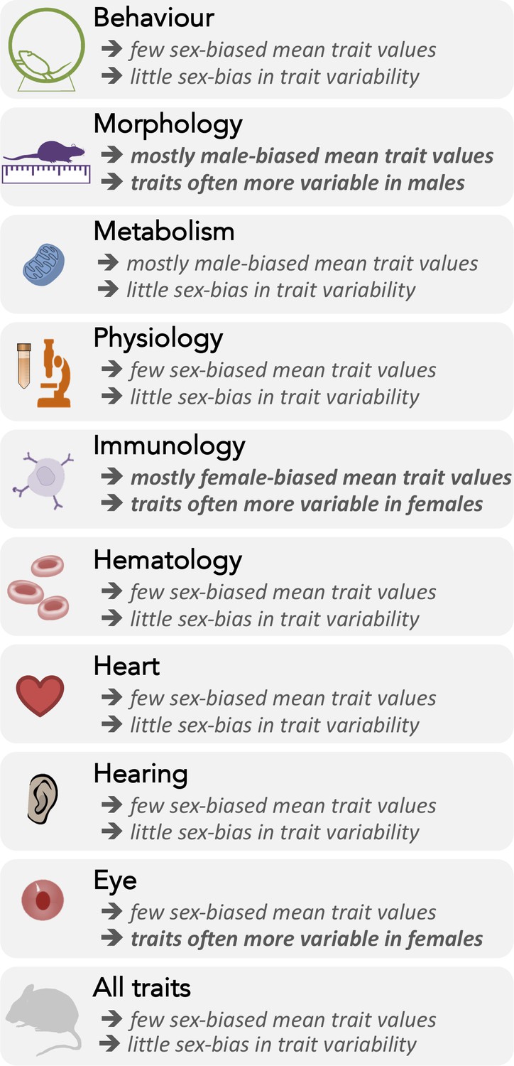
Summary of sex differences in the mean trait values (lnRR) and variances (lnCVR) across nine functional trait groups, and overall.
The estrus-mediated variability hypothesis was, at least until recently (Prendergast et al., 2014; Smarr et al., 2017), regularly used as a rationale for including only male subjects in many biomedical studies. So far, we know very little about the relationship between hormonal fluctuations and general trait variability within and among female subjects. Our results are consistent with the estrus-mediated variability hypothesis for immunological traits only. Immune responses can strongly depend on sex hormones (Zuk and McKean, 1996; Grossman, 1989), which may explain higher female variability in these traits. However, if estrus status affects traits through variation in hormone levels, we would expect to also find higher female variability in physiological and hematological traits. This was not the case in our dataset. Interestingly, however, eye morphology (structural traits, which should fluctuate little across the estrous cycle) also appeared to be more variable in females than males, but little is known about sex differences in ocular traits in general (Wagner et al., 2008; Shaqiri et al., 2018). Overall, we find no consistent support for the female estrus-mediated variability hypothesis.
In line with our findings, recent studies have refuted the prediction of higher female variability (Prendergast et al., 2014; Smarr et al., 2017; Beery and Zucker, 2011; Becker et al., 2016; Beery, 2018). For example, several rodent studies have found that males are more variable than females (Prendergast et al., 2014; Smarr et al., 2017; Becker et al., 2016; Beery, 2018; Fritz et al., 2017; Mogil and Chanda, 2005). Further studies should investigate whether higher female variability in immunological traits is indeed due to the estrous cycle, or generally because of greater between-individual variation (Figure 2).
In general, we found many traits to be sexually dimorphic (Figure 5) in accordance with the previous study, which used the same database (Karp et al., 2017). Although the original study also provided estimates for sex differences in traits both with and without controlling for weight (we did not control for weight; Nakagawa et al., 2017). More specifically, males are larger than females, while females have higher immunological parameters (see Figure 5). Notably, the most sexually dimorphic trait means also show the greatest differences in trait variance (Figures 4 and 5). Indeed, theory predicts that sexually selected traits (e.g. larger body size for males due to male-male competition) are likely more variable, as these traits are often condition-dependent (Rowe and Houle, 1996). Therefore, this sex difference in variability could be more pronounced under natural conditions compared to laboratory settings. This relationship may explain why male-biased morphological traits are larger and more variable.
Eco-evolutionary implications
We have used lnCVR values to compare phenotypic variability (CV) between the sexes. When lnCVR is used for fitness-related traits, it can signify sex differences in the ‘opportunity for selection’ between females and males (Rowe and Houle, 1996). If we assume that phenotypic variation (i.e. variability in traits) has a heritable basis, then large ratios of lnCVR may indicate differences in the evolutionary potential of each sex to respond to selection, at least in the short term (Hansen and Houle, 2008). For example, more variable morphological traits of males could potentially provide them with better capacity than females to adapt morphologically to a changing climate. We note, however, that in our study, lnCVR reflects sex differences in trait variability within strains, such that the variability differences we observe between the sexes may be partially the result of phenotypic plasticity.
Demographic parameters, such as age-dependent mortality rate (Lemaître et al., 2020) can often be different for each sex. For example, a study on European sparrowhawks found that variability in mortality was higher in females compared to males (Colchero et al., 2017). In this species, sex-specific variation affects age-dependent mortality and results in higher average female life expectancy. Therefore, population dynamic models, which make predictions about how populations change in their size over time, should take sex differences in variability into account to produce more accurate predictions (Caswell and Weeks, 1986; Lindström and Kokko, 1998). In our rapidly changing world, better predictions on population dynamics are vital for understanding whether climate change is likely to result in population extinction and lead to further biodiversity loss.
Statistical and practical implications
It is now mandatory to include both sexes in biomedical experiments and clinical trials funded by the NIH, unless there exists strong justification against the inclusion of both sexes (NIH, 2015a; NIH, 2015b). In order to conduct meaningful research and make sound clinical recommendations for both male and female patients, it is necessary to understand both how trait means and variances differ between the sexes. If one sex is systematically more variable in a trait of interest than the other, then experiments should be designed to accommodate relative differences in statistical power between the sexes (which has not been considered before, see Flanagan, 2014; Klein et al., 2015; Prendergast et al., 2014; Shansky and Woolley, 2016). For example, female immunological traits are generally more variable (i.e. having higher CV and SD). Therefore, in an experiment measuring immunological traits, we would need to include a larger sample (N) of females than males (N[female] > N[male]; N[total] = N[female] + N[male]) to achieve the same power as when the experiment only includes males (N[total*] = 2N[male]). In other words, in an experiment with both sexes we would need a larger sample size than the same experiment with males only (N[total] > N[total*]).
To help researchers adjust their sex-specific sample size to achieve optimal statistical power, we provide an online tool (ShinyApp; https://bit.ly/sex-difference). This tool may serve as a starting point for checking baseline variability for each sex in mice. The sex bias (indicated by the % difference between the sexes) is provided for separate traits, procedures, and functional groups. These meta-analytic results are based on our analyses of more than 2 million rodent data points, from 26,916 individual mice. We note, however, that variability in a trait measured in untreated individuals maintained under carefully standardized environmental conditions, as reported here, may not directly translate into the same variability when measured in experimentally treated individuals, or individuals exposed to a range of environments (i.e. natural populations or human cohorts). Further, these estimates are overall mean differences across strains and locations. Therefore, these may not be particularly informative if one’s experiment only includes one specific strain. Nonetheless, we point out that our estimates may be useful in the light of a recent recommendation of using ‘heterogenization’ where many different strains are systematically included (i.e. randomized complete block design) to increase the robustness of experimental results (Voelkl et al., 2020). However, note that an experiment with heterogenization might only include a few strains with several animals per strain. Even in such a case, using just a few strains, our tool could provide potentially useful benchmarks. Incidentally, heterogenization would be key to making one’s experimental outcome more generalizable (Webster and Rutz, 2020).
Importantly, when two groups (e.g. males and females) show differences in variability, we violate homogeneity of variance or homoscedasticity assumptions. Such a violation is detrimental because it leads to a higher Type I error rate. Therefore, we should consider incorporating heteroscedasticity (different variances) explicitly or using robust estimators of variance (also known as ‘the sandwich variance estimator’) to prevent an inflated Type I error rate (Cleasby and Nakagawa, 2011), especially when we compare traits between the sexes.
Conclusion
We have shown that sex biases in variability occur in many mouse traits, but that the directions of those biases differ between traits. Neither the ‘greater male variability’ nor the ‘estrus-mediated variability’ hypothesis provides a general explanation for sex differences in trait variability. Instead, we have found that the direction of the sex bias varies across traits and among trait types (Figures 4 and 5). Our findings have important ecological and evolutionary ramifications. If the differences in variability correspond to the potential of each sex to respond to changes in specific environments, this sex difference needs to be incorporated into demographic and population dynamic modelling. Moreover, in the (bio-)medical field, our results should inform decisions during study design by providing more rigorous power analyses that allow researchers to incorporate sex-specific differences for sample size. We believe that taking sex differences in trait variability into account will help avoid misleading conclusions and provide new insights into sex differences across many areas of biological and bio-medical research. Ultimately, such considerations will not only better our knowledge, but also close the current gaps in our biased knowledge (Tannenbaum et al., 2019).
Materials and methods
Data selection and process
Request a detailed protocolThe IMPC (International Mouse Phenotyping Consortium) provides a comprehensive catalogue of mammalian gene function for investigating the genetics of health and disease, by systematically collecting phenotypes of knock-out and wildtype mice. To investigate differences in trait variability between the sexes, we only considered the data for wildtype control mice. We retrieved the dataset from the IMPC server in June 2018 and filtered it to contain non-categorical traits for wildtype mice. The initial dataset comprised over 2,500,000 data points for 340 traits. In cases where multiple measurements were taken over time, data cleaning started with selecting single measurements for each individual and trait. In these cases, we selected the measurement closest to ‘100 days of age’. All data are from unstaged females (with no information about the stage of their estrous cycle). We excluded data for juvenile and unsexed mice (Figure 3A; this dataset and scripts can be found on https://rpubs.com/SusZaj/ESF; https://bit.ly/code-mice-sex-diff; raw data: https://doi.org/10.5281/zenodo.3759701).
Grouping and effect-size calculation
Request a detailed protocolWe created a grouping variable called ‘population’ (Figure 3B). A population comprised a group of individuals belonging to a distinct wildtype strain maintained at one particular location (institution); populations were identified for every trait of interest. Our data were derived from 11 different locations/institutions, and a given location/institution could provide data on multiple populations (see Supplementary file 1, Table 1 for details on numbers of strains and institutions). We included only populations that contained data points for at least six individuals, and which had information for members of both sexes; further, populations for a particular trait had to come from at least two institutions to be eligible for inclusion. After this selection process, the dataset contained 2,300,000 data points across 232 traits. Overall, we meta-analysed traits with between 2–18 effect sizes (mean = 9.09 effects, SD = 4.47). However, each meta-analysis contained a total number of individual mice that ranged from 83/91 to 13467/13449 (males/females). While a minimum of N = 6 mice were used to create effect sizes for any given group (male or female), in reality samples sizes of male/female groups were much larger (males: mean = 396.66 (SD = 238.23), median = 465.56; females: mean = 407.35 (SD = 240.31), median = 543.89). We used the function escalc in the R package, metafor (Viechtbauer, 2010) to obtain lnCVR, lnVR and lnRR and their corresponding sampling variance for each trait for each population; we worked in the R environment for data cleaning, processing and analyses (R Development Core Team, 2017, version 3.6.0; for the versions of all the software packages used for this article and all the details and code for the statistical analyses, see Source code 1 and repositories). As mentioned above, the use of ratio-based effect sizes, such as lnCVR, lnVR and lnRR, controls for baseline changes over time and space, assuming that these changes affect males and females similarly. However, we acknowledge that we could not test this assumption.
Meta-analyses: overview
Request a detailed protocolWe conducted meta-analyses at two different levels (Figure 3C–J). First, we conducted a meta-analysis for each trait for all three effect-size types (lnRR, lnVR and lnCVR), calculated at the ‘population’ level (i.e. using population as a unit of analysis). Second, we statistically amalgamated overall effect sizes estimated at each trait (i.e. overall trait means as a unit of analysis) after accounting for dependence among traits. In other words, we conducted second-order meta-analyses (Nakagawa et al., 2019). We used the second-order meta-analyses for three different purposes: (A) estimating overall sex biases in variance (lnCVR and lnVR) and mean (lnRR) in the nine functional groups (for details, see below) and in all these groups combined (the overall estimates); (B) visualizing heterogeneities across populations for the three types of effect size in the nine functional trait groups, which complemented the first set of analyses (Figure 3I, Table 6 in Supplementary file 1); and (C) when traits were found to be significantly sex-biased, grouping such traits into either male-biased and female-biased traits, and then, estimating overall magnitudes of sex bias for both sexes again for the nine functional trait groups. Only the first second-order meta-analysis (A) directly related to the testing of our hypotheses, results of B and C are found in Supplementary file 1 and figures and reported in our freely accessible code.
Meta-analyses: population as an analysis unit
Request a detailed protocolTo obtain degree of sex bias for each trait mean and variance (Figure 3C), we used the function rma.mv in the R package metafor (Viechtbauer, 2010) by fitting the following multilevel meta-analytic model, an extension of random-effects models (sensu Nakagawa and Santos, 2012):
ESi ~ 1 + (1 | Strainj) + (1 | Locationk) + (1 | Uniti) + Errori, where ‘ESi’ is the ith effect size (i.e. lnCVR, lnVR and lnRR) for each of 232 traits, the ‘1’ is the overall intercept (other ‘1’s are random intercepts for the following random effects), ‘Strainj’ is a random effect for the jth strain of mice (among nine strains), ‘Locationk’ is a random effect for the kth location (among 11 institutions), ‘Uniti’ is a residual (or effect-size level or ‘population-level’ random effect) for the ith effect size, ‘Errori’ is a random effect of the known sampling error for the ith effect size. Given the model above, meta-analytic results had two components: (1) overall means with standard errors (95% confidence intervals), and (2) total heterogeneity (the sum of the three variance components, which is estimated for the random effects). Note that overall means indicate average (marginalised) effect sizes over different strains and locations, and total heterogeneities reflect variation around overall means due to different strains and locations.
We excluded traits which did not carry useful information for this study (i.e. fixed traits, such as number of vertebrae, digits, ribs and other traits that were not variable across wildtype mice; note that this may be different for knock-down mutant strains) or where the meta-analytic model for the trait of interest did not converge, most likely due to small sample size from the dataset (14 traits, see SI Appendix, for details: Meta-analyses; 1. Population as analysis unit). We therefore obtained a dataset containing meta-analytic results for 218 traits, at this stage, to use for our second-order meta-analyses (Figure 3D).
Meta-analyses: accounting for correlated traits
Request a detailed protocolOur dataset of meta-analytic results included a large number of non-independent traits. To account for dependence, we identified 90 out of 218 traits, and organized them into 19 trait sub-groups (containing 2–10 correlated traits, see Figure 3E). For example, many measurements (i.e. traits) from hematological and immunological assays were hierarchically clustered or overlapped with each other (e.g. cell type A, B and A+B). We combined the meta-analytic results from 90 traits into 19 meta-analytic results (Figure 3F) using the function robu in the R package robumeta with the assumption of sampling errors being correlated with the default value of r = 0.8 (Fisher et al., 2017). Consequently, our final dataset for secondary meta-analyses contained 147 traits (i.e. the newly condensed 19 plus the remaining 128 independent traits, see Figure 3, Supplementary file 1, Table 2), which we assume to be independent of each other.
Second-order meta-analyses: trait as an analysis unit
Request a detailed protocolWe created our nine overarching functional groups of traits (Figure 3G) by condensing the IMPC’s 26 procedural categories (‘procedures’) into related clusters. The categories were based on procedures that were biologically related, in conjunction with measurement techniques and the number of available traits in each category (see Supplementary file 1, Table 3 for a list of clustered traits, procedures and grouping terms). To test our two hypotheses about how trait variability changes in relation to sex, we estimated overall effect sizes for nine functional groups by aggregating meta-analytic results via ‘classical’ random-effect models using the function rma.uni in the R package metafor (Viechtbauer, 2010). In other words, we conducted three sets of 10 second-order meta-analyses (i.e. meta-analyzing 3 types of effect size: lnRR, lnVR and lnCVR for nine functional groups and one for all the groups combined, Figure 3H). Although we present the frequencies of male- and female-biased traits in Figure 4A, we did not run inferential statistical tests on these counts because such tests would be considered as vote-counting, which has been severely criticised in the meta-analytic literature (Higgins, 2019).
Data availability
The code and data generated during this study are freely accessible on GitHub. (https://github.com/itchyshin/mice_sex_diff; copy archived at https://archive.softwareheritage.org/swh:1:rev:2868f59b32d05a61091e70962e6e6a16463c6a64/) as well as OSF (https://osf.io/25h4t/). Original/source data (pre-cleaned dataset as downloaded from IMPC) can be downloaded from zenodo (DOI:10.5281/zenodo.3759701). The supporting files also contain the full code workflow.
-
ZenodoRaw data for: Sex and Power: Sexual dimorphism in trait variability and its eco-evolutionary and statistical implications.https://doi.org/10.5281/zenodo.3759701
References
-
Inclusion of females does not increase variability in rodent research studiesCurrent Opinion in Behavioral Sciences 23:143–149.https://doi.org/10.1016/j.cobeha.2018.06.016
-
Sex bias in neuroscience and biomedical researchNeuroscience & Biobehavioral Reviews 35:565–572.https://doi.org/10.1016/j.neubiorev.2010.07.002
-
Two-Sex models: chaos, extinction, and other dynamic consequences of sexThe American Naturalist 128:707–735.https://doi.org/10.1086/284598
-
Studying both sexes: a guiding principle for biomedicineThe FASEB Journal 30:519–524.https://doi.org/10.1096/fj.15-279554
-
Neglected biological patterns in the residualsBehavioral Ecology and Sociobiology 65:2361–2372.https://doi.org/10.1007/s00265-011-1254-7
-
Phenotypic variation and fluctuating asymmetry in sexually dimorphic feather ornaments in relation to sex and mating systemBiological Journal of the Linnean Society 68:505–529.https://doi.org/10.1111/j.1095-8312.1999.tb01186.x
-
The descent of man and Selection in Relation to SexJournal of Anatomy and Physiology 5:363–372.
-
Intrinsic excitability varies by sex in prepubertal striatal medium spiny neuronsJournal of Neurophysiology 113:720–729.https://doi.org/10.1152/jn.00687.2014
-
Sexual dimorphism in biomedical research: a call to analyse by sexTransactions of the Royal Society of Tropical Medicine and Hygiene 108:385–387.https://doi.org/10.1093/trstmh/tru079
-
Sex differences in the anorexigenic effects of dexfenfluramine and amphetamine in baboonsExperimental and Clinical Psychopharmacology 26:335–340.https://doi.org/10.1037/pha0000201
-
Similar reliability and equivalent performance of female and male mice in the open field and water-maze place navigation taskAmerican Journal of Medical Genetics Part C: Seminars in Medical Genetics 175:380–391.https://doi.org/10.1002/ajmg.c.31565
-
Possible underlying mechanisms of sexual dimorphism in the immune response, fact and hypothesisJournal of Steroid Biochemistry 34:241–251.https://doi.org/10.1016/0022-4731(89)90088-5
-
Measuring and comparing evolvability and constraint in multivariate charactersJournal of Evolutionary Biology 21:1201–1219.https://doi.org/10.1111/j.1420-9101.2008.01573.x
-
Sex differences in variability in general intelligence: a new look at the old questionPerspectives on Psychological Science 3:518–531.https://doi.org/10.1111/j.1745-6924.2008.00096.x
-
Prevalence of sexual dimorphism in mammalian phenotypic traitsNature Communications 8:15475.https://doi.org/10.1038/ncomms15475
-
Sexual reproduction and population dynamics: the role of polygyny and demographic sex differencesProceedings of the Royal Society of London. Series B: Biological Sciences 265:483–488.https://doi.org/10.1098/rspb.1998.0320
-
Meta‐analysis of variation: ecological and evolutionary applications and beyondMethods in Ecology and Evolution 6:143–152.https://doi.org/10.1111/2041-210X.12309
-
Research weaving: visualizing the future of research synthesisTrends in Ecology & Evolution 34:224–238.https://doi.org/10.1016/j.tree.2018.11.007
-
Methodological issues and advances in biological meta-analysisEvolutionary Ecology 26:1253–1274.https://doi.org/10.1007/s10682-012-9555-5
-
ReportConsideration of Sex as a Biological Variable in NIH-Funded Research, Notice NOT-OD-102National Institutes of Health.
-
ReportEnhancing Reproducibility Through Rigor and Transparency, Notice NOT-OD-103National Institutes of Health.
-
A resolution of the lek paradoxProceedings of the Royal Society of London. Series B, Containing Papers of a Biological Character 260:21–29.https://doi.org/10.1098/rspb.1995.0054
-
Female mice liberated for inclusion in neuroscience and biomedical researchNeuroscience & Biobehavioral Reviews 40:1–5.https://doi.org/10.1016/j.neubiorev.2014.01.001
-
SoftwareR: A Language and Environment for Statistical ComputingR Foundation for Statistical Computing, Vienna, Austria.
-
Sex-Dependent intestinal replication of an enteric virusJournal of Virology 91:e02101-16.https://doi.org/10.1128/JVI.02101-16
-
The lek paradox and the capture of genetic variance by condition dependent traitsProceedings of the Royal Society B: Biological Sciences 263:1415–1421.https://doi.org/10.1098/rspb.1996.0207
-
Revisiting and expanding the meta-analysis of variation: the log coefficient of variation ratioResearch Synthesis Methods 11:553–567.https://doi.org/10.1002/jrsm.1423
-
Considering sex as a biological variable will be valuable for neuroscience researchThe Journal of Neuroscience 36:11817–11822.https://doi.org/10.1523/JNEUROSCI.1390-16.2016
-
Sex differences in variability across timescales in BALB/c miceBiology of Sex Differences 8:3.https://doi.org/10.1186/s13293-016-0125-3
-
Prenatal hypoxia impairs cardiac mitochondrial and ventricular function in guinea pig offspring in a sex-related mannerAmerican Journal of Physiology. Regulatory, Integrative and Comparative Physiology 315:R1232–R1241.https://doi.org/10.1152/ajpregu.00224.2018
-
Genic capture and resolving the lek paradoxTrends in Ecology & Evolution 19:323–328.https://doi.org/10.1016/j.tree.2004.03.029
-
Conducting Meta-Analyses in R with the metafor PackageJournal of Statistical Software 36:i03.https://doi.org/10.18637/jss.v036.i03
-
Reproducibility of animal research in light of biological variationNature Reviews Neuroscience 21:384–393.https://doi.org/10.1038/s41583-020-0313-3
-
Sex- and gender-based differences in healthy and diseased eyesOptometry - Journal of the American Optometric Association 79:636–652.https://doi.org/10.1016/j.optm.2008.01.024
-
Sex differences in pharmacokinetics predict adverse drug reactions in womenBiology of Sex Differences 11:32.https://doi.org/10.1186/s13293-020-00308-5
-
Sex differences in parasite infections: patterns and processesInternational Journal for Parasitology 26:1009–1024.https://doi.org/10.1016/S0020-7519(96)80001-4
Decision letter
-
Christian RutzSenior Editor; University of St Andrews, United Kingdom
-
Rosalyn GloagReviewing Editor; University of Sydney, Australia
-
Rosalyn GloagReviewer; University of Sydney, Australia
In the interests of transparency, eLife publishes the most substantive revision requests and the accompanying author responses.
Acceptance summary:
This study makes a valuable contribution to our understanding of sex-differences in trait variability. It applies a meta-analytic approach to mouse datasets to test two hypotheses of sex-specific variability in mammals: that females show greater variability due to estrous, and that males show greater variability due to heterogamy and/or sexual selection. It reveals that, at least for mice, neither hypothesis is universally true for all traits. Rather, variability is greater in females for some traits, and greater in males for others. These interesting results provide new insights into sex bias in variability, that will inform experimental design in diverse biological fields.
Decision letter after peer review:
[Editors’ note: the authors submitted for reconsideration following the decision after peer review. What follows is the decision letter after the first round of review.]
Thank you for submitting your work entitled "Sex and Power: sexual dimorphism in trait variability and its eco-evolutionary and statistical implications" for consideration by eLife. Your article has been reviewed by three peer reviewers, including Rosalyn Gloag as the Reviewing Editor and Reviewer #1, and the evaluation has been overseen by a Senior Editor. The following individual involved in the review of your submission has agreed to reveal their identity: Irving Zucker (Reviewer #3).
Our decision has been reached after consultation between the reviewers. Based on these discussions, and the individual reviews appended below, we regret to inform you that your work in its current form is not suitable for publication in eLife.
All reviewers agreed that the topic of the study was an interesting one, and that the issue of sex differences in trait variability is relevant to good experimental design. As you'll see below, however, reviewer #2 felt that the current analytical treatment of this mouse dataset is not appropriate to the question. Of particular concern is that sources of variability other than sex were not adequately considered. We recommend that this issue, and others outlined in the reviews below, are carefully addressed in any revision. Given the interest in the topic, we are prepared to reconsider a thoroughly revised version of the manuscript, if you think you can adequately address the concerns raised, but please note that this does not guarantee formal re-evaluation let alone eventual acceptance.
Reviewer #1:
This study looks at whether there are sex differences in the variability of traits in mice, via a meta-analysis of published datasets. The analyses show that females typically show greater variability in traits categorised as immunological, while males show greater variability in morphological traits. Traits related to the eye were also more variable in females. These findings are interpreted in light of evolutionary theory about greater between-individual variability in males, and greater within-individual variability in female mammals due to estrus. A online tool is provided to allow researchers to consider possible sex-specific variability in traits at the experimental design phase.
I enjoyed the paper and thought the question and conclusions were interesting. The figures are great. I am not an expert in meta-analyses, nor in mice, so my comments mostly relate to the hypotheses and discussion of the results.
1) The paper jumps about quite a bit between talking about sex differences relevant to mammals only and those that might apply to animals more generally. For example, the Introduction begins with reference to biomedical research (mammals) and the estrus hypothesis (mammals) but then introduces the "male variability" hypothesis by stating the "males are often the heterogametic sex". Given that the subject of your study is the mouse, I think it would be more logical to restrict the Introduction to mammals (i.e. explain the two hypotheses with respect to mammals). You could then include a section in the Discussion on if/why we might expect the same trends in other animals (see below also).
2) I feel that the rationale behind the two hypotheses (female estrus and male variability) could be explained better in the Introduction. i.e. why estrus might produce higher variability in females and why stronger sexual selection or male heterogamety might produce greater male variability. A few extra sentences on each would probably be enough. At the same time, I think it would be worth clarifying a priori the extent to which these hypotheses are expected to apply to different traits. Some predictions are given only in the Discussion (e.g. estrus expected to mostly affect immune response and physiology).
3) The Discussion on eco-evolutionary implications would be greatly strengthened if it included at least one specific example of how sex-specific differences in trait variability might affect the evolutionary trajectory of a population. At present, one very general hypothetical is given, but I did not find it easy to follow (disease/climate change kills more of one sex than the other –> sex ratio of the population is skewed (temporarily?) –> mating system is "influenced" –> "downstream affects on population dynamics"). It is also stated that "modelling sex difference in trait variability could lead to different conclusions compared to existing models (cf 44)". The cited study there is on Eurasian sparrowhawks. I'm not familiar with this sparrowhawk study, but perhaps it is a suitable one to highlight in more detail as a clear example? What sort of different conclusions would be expected? It's great that your paper is aiming to speak to a broad range of biologists, but I think that greater clarity in this section is needed to make ecologists and evolutionary biologists really take notice.
Reviewer #2:
Summary
There are significant methodology and interpretative concerns with this article. The analysis over stretches and does not consider the potential weaknesses. It needs to refocus on the primary question of whether there is a pattern in the sex's impact on the variance for these traits. The analysis then needs to go deeper and remove other sources of variance that could be confounding their findings.
Methodology
1) The methodology is not clear.
2) Meta-analysis is used when you don't have access to the raw data – why not use mixed effect regression models?
3) The variance summary metric is calculated for an institute and strain for data collected in multiple batches, with potential baseline shifts as the data is collected across many years. This isn't a representative metric of variability for a sex as there are multiple sources of variance impacting this metric.
4) Figure 3B and code: It is very rare for a fixed effect analysis to be justifiable. Why assume that there is no variation between the different traits when testing effect of sex? Normally you would explore sources of heterogeneity by meta regression rather than just assume it is sex differences.
5) "A previous study found that the heterogametic sex was more variable in body size". If this holds, would not traits that are correlated with body weight also demonstrate the same finding?
6) "minimum of 2 different institutes" is a very low N. Why would this give meaningful analysis? What was the minimum amount of data for a strain*centre for a trait to be included?
7) Consider the recent discussions on phenotypic plasticity and the phenotypic interaction with the environment (https://www.nature.com/articles/s41583-020-0313-3). This suggests a fixed effect model is not appropriate. The results and approach need discussing in this context.
Conclusion
1) It isn't made clear that this analysis is trying to assess the role of sex across strains and institutes.
2) There is no discussion of the potential weakness of the analysis.
3) Figure 3A:
– Why is there no discussion of measures of heterogeneity within the meta-analysis at the population level?
– Should the differences in classification as male or female biased within functional group not be assessed by a fisher exact test and the p value adjusted for multiple testing before you state an area has a difference?
4) Concern by "Notably most SD trait means also show the greater difference in trait variance" – seems to be an eyeball rather than a statistical analysis.
5) I have concerns on relating these results to power:
– These estimates are from an analysis across strains, batches and institutes looking at global behaviour in the traits. This absolute variance measure would be very different to that seen in a lab within a classic parallel group design study with one strain.
– They advocate a factorial design but suggest the powering of the sexes independently. This feeds into the misconception that to study both sexes you have to double your sample size.
6) The authors report that this analysis on mean differences was in accordance with previous studies. Not really. The differences will arise from the different approaches taken and highlights how this summary metric is losing sensitivity. The authors relate many of these changes to a difference in body size. However, the earlier published analysis, adjusted for body weight.
7) Why would the "difference in variability impact on the potential of each sex to respond to changes in specific environments"?
Reviewer #3:
This is a comprehensive meta-analysis of empirical literature on sex differences in mammalian trait variability. The authors nicely articulate competing hypotheses: "estrus-mediated variability" (which predicts higher trait variability in females because they exhibit cyclic reproductive [estrous] hormone secretion that occurs over multi-day timescales) vs. "male variability hypothesis" (which predicts higher trait variability in males because they are the heterogametic sex). Several prior meta-analyses related to this have not provided support for the estrus-mediated variability hypothesis. The analysis performed here differs significantly from prior work in that the subjects were 27,147 mice from the International Mouse Phenotyping Consortium, which generated over 2x10⁶ data points. Unlike other meta-analyses, the subjects of this analysis were therefore more systematically evaluated (9 wildtype strains across 11 labs). A total of 218 continuous traits were evaluated, grouped into 9 functional trait groups. Some traits were biased towards males and others towards females. There was no consistent pattern of greater variability in either sex. The results support a straightforward conclusion that neither hypothesis adequately explains patterns of trait variability. the discussion is a restrained defense of the practice of including females (please clarify that monitoring of estrous cycles was not performed in these studies so the females are classified as as "unstaged"); consequently females can be included in research studies without a default assumption that they are any more likely to introduce more variability than including males. The authors also apply their data on widespread differences in trait specific lnCVR values to the potential for phenotypic response to selection due to rapidly changing environmental events. The Discussion is well written with the sections that are each meaningful. The web-based tool is a very helpful contribution. The discussion of statistical implications of the work (e.g., equalizing power and Type I consequences of unequal variance) is of significance to research on mammalian biology.
1) The present work adds important new information to a growing literature (see for example Smarr BL, Rowland NE Zucker I. Male and female mice show equal variability in food intake across 4-day spans that encompass estrous cycles. PLoS One. 2019 Jul 15;14(7):e0218935) indicating that incorporation of unstaged female rodents in biomedical research does not increase variability compared to that generated by males; importantly, it also specifies several circumstances in which specific traits are more variable in one sex than the other.
2) The statement “ This higher trait variability, resulting from females being at
different stages of their estrous cycle, is the main reason for why female research subjects are often excluded from biomedical research trials, especially in the neurosciences, physiology and pharmacology” is a strong overgeneralization and should be tempered and/or clarified: "However, scientists in (bio-)medical fields have not traditionally regarded sex as a biological factor of intrinsic interest (2-7)." This is an overstatement. The study of sex differences and sexual differentiation in mammals (a class of animals of most direct relevance to biomedical research) has a long history, complete with dedicated journals (e.g. Biology of Sex Differences), learned societies, etc. Such an enduring interest in sex among biologists only makes the present work more interesting and important. This critique may be addressed with a more clear definition of "(bio-)medical", here, and throughout the manuscript.
3) Colloquialisms such as "This is an important step, but we can go much further" are vague and difficult for this reader to endorse as true, as written and we recommend deletion.
4) In the Introduction, the authors delineate competing hypotheses: "estrus-mediated variability" vs. "male variability hypothesis". In their elaboration of the former hypothesis, the authors should clarify that the historical concern regarding decreased power and increased variability in females compared to males specifically regarded the inclusion of females that were not synchronized (or "staged") so as to be tested/treated on the same day/phase of the estrous cycle. Data from these so-called “randomly cycling” females were predicted to be more variable than data from males. "Staged" females were presumed to be less variable, and the interventions and costs associated with the presumed need for staging are viewed as onerous. But a growing literature, including the important new results from the present study, argues that there is no empirical support for the contention that females generally are more variable than males across many traits.
5) Materials and methods: the data analysis pipeline is clear and rigorous. It should be stated that the data used come from unstaged females.
[Editors’ note: further revisions were suggested prior to acceptance, as described below.]
Thank you for resubmitting your work entitled "Sexual dimorphism in trait variability and its eco-evolutionary and statistical implications" for further consideration by eLife. Your revised article has been evaluated by a Senior Editor, a Reviewing Editor, and a reviewer.
The manuscript has been improved, but three issues were raised in this second round of review that need to be addressed before final acceptance:
1) Please ensure that the proposal for sample heterogenization by Voelkl et al., 2020, is not misrepresented in your discussion. In that review, the authors do recommend heterogenization but not in an uncontrolled fashion, rather a systematic inclusion of variation with a randomised block design. If there is only one replicate per treatment per block then, yes, the variance measured in this manuscript (and hence app) will be a good representation of the variance expected. This type of design is likely to be rare and most researchers will use a RBD with replication within a block and less strains. Please carefully revise your manuscript to avoid suggesting that the recommendation is to mix different strains (as that isn't quite correct).
2) Regarding the powering of studies, you state: "If we assume that responses to an experimental treatment will be similar between the sexes for this functional trait group, we will require more females to achieve the same statistical power as for the males." The wording here implies that the power calculations for a treatment effect are calculated separately for the males and the females. This reinforces the misconception that when you study both sexes you should consider the powering as two independent randomised complete designs (and hence if the variance is equal you would double the sample size). As you are talking about designs which include both sexes (not the selection of one versus the other), there is a need to explicitly state that power in a factorial design is achieved by assessment of the treatment effect from both the males and the females. If the variance is different between the sexes, there is a need to increase the N in the more variable sex to achieve the same final sensitivity.
3) While the Discussion section on "eco-evolutionary implications" is improved, this section still lacks clarity, the second paragraph in particular. What are "population dynamic models" and why are they important? What "different conclusions" are alluded to when you state, "explicitly modelling sex difference in trait variability could lead to different conclusions compared to traditional modelling approaches"? There is also no longer any mention of climate change in this paragraph, even though it is mentioned in the Abstract as an example of an "eco-evolutionary ramification". These points need strengthening to justify the article's title and capture the attention of a wider range of biologists.
Finally, the editors of eLife have recently decided to adopt the STRANGE framework for animal-behaviour research (https://www.nature.com/articles/d41586-020-01751-5?sf235295265=1) and will shortly update the journal's author guidelines and transparent reporting form. Given the link between STRANGE and the topic of your article, please consider, if possible, in your final revision how your study might engage with this new framework.
https://doi.org/10.7554/eLife.63170.sa1Author response
[Editors’ note: the authors resubmitted a revised version of the paper for consideration. What follows is the authors’ response to the first round of review.]
Reviewer #1:
[…]
1) The paper jumps about quite a bit between talking about sex differences relevant to mammals only and those that might apply to animals more generally. For example, the Introduction begins with reference to biomedical research (mammals) and the estrus hypothesis (mammals) but then introduces the "male variability" hypothesis by stating the "males are often the heterogametic sex". Given that the subject of your study is the mouse, I think it would be more logical to restrict the Introduction to mammals (i.e. explain the two hypotheses with respect to mammals). You could then include a section in the Discussion on if/why we might expect the same trends in other animals (see below also).
This is a great suggestion. We have changed the corresponding paragraph accordingly; now this reads:
“Second, the “greater male variability hypothesis” suggests males exhibit higher trait variability because of two different mechanisms. The first mechanism is based on males being the heterogametic sex in mammals...”
2) I feel that the rationale behind the two hypotheses (female estrus and male variability) could be explained better in the Introduction. i.e. why estrus might produce higher variability in females and why stronger sexual selection or male heterogamety might produce greater male variability. A few extra sentences on each would probably be enough. At the same time, I think it would be worth clarifying a priori the extent to which these hypotheses are expected to apply to different traits. Some predictions are given only in the Discussion (e.g. estrus expected to mostly affect immune response and physiology).
We realise that we were too concise in the original manuscript. We have added additional explanations to the estrous cycle hypothesis:
“…. A wide range of labile traits are presumed to co-vary with physiological changes that are induced by reproductive hormones. High variability is, therefore, expected to be particularly prominent when the stage of the estrous cycle is unknown and unaccounted for. This higher trait variability, resulting from females being at different stages of their estrous cycle, is the main reason for why female research subjects are often excluded from biomedical research trials, especially in the neurosciences, physiology and pharmacology. …”
And the male variability hypothesis:
“Second, the “greater male variability hypothesis” suggests males exhibit higher trait variability because of two different mechanisms. […] So far, the “greater male variability hypothesis” has gained some support in the evolutionary and psychological literature.”
Because we had no a priori expectations regarding which traits would be differently affected, this is not expanded upon in the Introduction. In fact, we had expected to find overarching support for either higher male or higher female variability, which was not supported by the data.
3) The Discussion on eco-evolutionary implications would be greatly strengthened if it included at least one specific example of how sex-specific differences in trait variability might affect the evolutionary trajectory of a population. At present, one very general hypothetical is given, but I did not find it easy to follow (disease/climate change kills more of one sex than the other –> sex ratio of the population is skewed (temporarily?) –> mating system is "influenced" –> "downstream effects on population dynamics"). It is also stated that "modelling sex difference in trait variability could lead to different conclusions compared to existing models". The cited study there is on Eurasian sparrowhawks. I'm not familiar with this sparrowhawk study, but perhaps it is a suitable one to highlight in more detail as a clear example? What sort of different conclusions would be expected? It's great that your paper is aiming to speak to a broad range of biologists, but I think that greater clarity in this section is needed to make ecologists and evolutionary biologists really take notice.
We have rewritten the entire paragraph to strengthen our eco-evolutionary implications:
“Demographic parameters, such as age-dependent mortality rate, are often different for each sex. Indeed, recognition of this fact has resulted in population dynamic models taking these widely observed sex differences into account. For example, a study on European sparrowhawks found that variability in mortality was higher in females compared to males. In this species, sex-specific variation affects age-dependent mortality and results in higher female life expectancy. As such, explicitly modelling sex difference in trait variability could lead to different conclusions compared to traditional modelling approaches.”
Reviewer #2:
Summary
There are significant methodology and interpretative concerns with this article. The analysis over stretches and does not consider the potential weaknesses. It needs to refocus on the primary question of whether there is a pattern in the sex's impact on the variance for these traits. The analysis then needs to go deeper and remove other sources of variance that could be confounding their findings.
Reviewer 2 has carefully read the code and its annotations, because s/he correctly points out our mistake in the annotation (see below; this html is an extensive document including a flow diagram of our data processing and statistical analyses based on >2,900 lines of code). Thus, we believe that reviewer 2’s concerns mainly stem from our omissions of some methodological descriptions and justifications in the original manuscript.
We have taken these criticisms seriously to further improve the clarity of our written methodology. In our revised version, we have clearly stated how our method deals with the confounders (see our replies below). By using a meta-analytical method (2nd comment by reviewer 2 – and we have expanded it there), many confounding effects have been taken care of. We do note, however, that our extended html was indeed helpful because reviewer 3 states “Materials and methods: the data analysis pipeline is clear and rigorous.”, which contrasts with what reviewer 2 says.
Methodology
1) The methodology is not clear.
We have endeavoured to make our methodology more accessible and comprehensive by addressing reviewer 2’s and the others’ comments. We would like to point out that we do have a methodological flowchart in our supplementary material as we were very much aware that our method is complex (and therefore, it might have been unclear). We have added more explanation in the main text and the supplement where possible (see our other replies to reviewer 2 below).
2) Meta-analysis is used when you don't have access to the raw data – why not use mixed effect regression models?
This is an important comment; it appears that our original version did not cover the justification for the approach clearly enough. However, in medicine, for example, a meta-analytic method like ours are often used even when one has raw data from different studies (i.e. individual patient data (IPD) meta-analyses, where they could also analyse raw data in these “meta-analyses”, rather than using summary effect sizes; see Debray et al., 2015, 6: p293, Res. Syn. Meth.). That aside, we have three main reasons why we used a meta-analytic approach (although the original manuscript omitted the second and third reasons – we have added this now, for exact wording see below).
First, as we wrote in the original manuscript: “Our meta-analytic approach allows easy interpretation and comparison with earlier and future studies.” This is because lnCVR and lnRR can be interpreted in terms of % differences between sexes (most of us have good intuitions for % differences compared to absolute differences in particular units, say, cm).
Second, and this is probably the most important reason, in the most common versions of mixed effect models, we cannot compare and contrast differences in variances between two groups. One possible way around this would be to model heteroskedasticity explicitly (see Cleasby and Nakagawa, 2011), which would require the specification and estimation of complex variance-covariance structure in the model residuals and introduce potential model identification problems. In any case, the approach we took using lnCVR, allows for a simpler and direct test of the research question. This is the main reason to use a meta-analytic approach.
Third, the use of standardised effect size, such as lnRR (log response ratio) or lnCVR, is sometimes referred to as the “contrast” method. This is because these effect sizes are the ratio of two effects between the treatment and control groups (females and males in our case). Taking a ratio has major advantages over modelling raw data, because it controls for different units across traits and it better controls for temporal and spatial changes in the traits themselves across control/treatment groups (here males and females; assuming that changes are relative). This is one of the biggest benefits of meta-analysis.
This “contrast” approach also addresses another part of the comment made by reviewer 2 in their opening paragraph that “It needs to refocus on the primary question of whether there is a pattern in the sex's impact on the variance for these traits. The analysis then needs to go deeper and remove other sources of variance that could be confounding their findings”. By taking the ratio within each study (i.e. relative to a concurrent control under matching conditions), the confounding effects are accounted for within each study and the effect size – and any potential effect on variance – is isolated. Thus, many experiment-specific factors do not need to be modelled explicitly; this is one of the arguments underlying conventional meta-analysis. The method used here (lnCVR) uses the same “contrast” approach and has the same advantages.
We now understand that our omissions of the second and third reasons made it difficult for reviewer 2 (and others) to assess the validity of our approach, generating concerns. Therefore, we have added these reasons to the manuscript:
“… Further, the proposed method using lnCVR (and lnVR) is probably the only practical method to compare variability between two sexes within and across studies, as far as we are aware. Also, the use of a ratio (i.e. lnRR, lnVR, lnCVR) between two groups (males and females) naturally controls for different units (e.g., cm, g, ml) and also for changes in traits over time and space.”
3) The variance summary metric is calculated for an institute and strain for data collected in multiple batches, with potential baseline shifts as the data is collected across many years. This isn't a representative metric of variability for a sex as there are multiple sources of variance impacting this metric.
As described above, lnCVR (like lnRR, lnVR, and Hedges’ g) is a contrast metric that is relative to a concurrent control under matching conditions. Assuming “potential baseline shifts” affect males and females equally, these variabilities are already taken care of when using ratio-based effect sizes. We now have mentioned this point in the Introduction (see above). Also, we had added this sentence in the Materials and methods section:
“As mentioned above, the use of ratio-based effect sizes such as lnCVR, lnVR and lnRR controls for baseline changes over time and space, assuming that these changes affect males and females similarly. However, we acknowledge that we could not test this assumption.”
4) Figure 3B and code: It is very rare for a fixed effect analysis to be justifiable. Why assume that there is no variation between the different traits when testing effect of sex? Normally you would explore sources of heterogeneity by meta regression rather than just assume it is sex differences.
We agree with reviewer 2 and we have to apologise for our mistake. We believe reviewer 2 thought we might have used fixed-effect models from the code annotation:
“# Final fixed effects meta-analyses within grouping terms”. This was an annotation mistake.
In the code, we ran random-effects meta-analyses throughout. Indeed, in our Materials and methods section of the original manuscript, we stated that we have used “random-effects” models and also multilevel models, which are a version of random-effects models (see Nakagawa et al., 2017).
“…, we estimated overall effect sizes for nine functional groups by aggregating meta-analytic results via a “classical” random-effect models using the function rma.uni in the R package metafor.”
This is for the second-order meta-analysis aggregating traits into groups of traits:
“we used the function rma.mv in the R package metafor (Viechtbauer, 2010) by fitting the following multilevel meta-analytic model, an extension of random-effects models (sensu Nakagawa & Santos 2012):
ESi ~ 1 + (1 |Strainj ) + (1 | Locationk) + (1 | Uniti) + Errori, ”
This is for each trait. As you can see, we are marginalising over strains and locations to get the average effect sizes for both lnRR (mean difference) and lnCVR (relative variance difference).
We thank reviewer 2 for spotting this mistake in code annotation, and now it has been corrected.
5) "A previous study found that the heterogametic sex was more variable in body size". If this holds, would not traits that are correlated with body weight also demonstrate the same finding?
Reviewer 2 would be correct if we were talking about mean differences (i.e. lnRR). We would expect, for example, traits, which correlate with body size, would show males have larger trait value in these traits. And this can be shown in our results of lnRR.
However, this will not necessarily be the case for differences in relative variance (i.e. lnCVR). This is because trait CVs do not necessarily correlate with trait means. This is the reason why we have provided % differences of CV (along with mean and SD) for all the traits we investigated via a Shiny App. The Shiny App will be useful for researchers to find which traits have potentially sex-biased CVs.
6) "minimum of 2 different institutes" is a very low N. Why would this give meaningful analysis? What was the minimum amount of data for a strain*centre for a trait to be included?
We are sorry that this was not clear. Despite having a minimum of two institutions, these institutions usually had replicated samples of mice from different experiments. In fact, we meta-analysed traits with between 2–18 effect sizes (mean = 9.09 effects, SD = 4.47); note that for Cochrane reviews, the median number of effect sizes per meta-analysis is 3 (so overall our meta-analyses have higher sample sizes than Cochrane reviews). While a minimum of N = 6 mice were used to create effect sizes for any given group (male or female), in reality samples sizes of male / female groups were much larger (males: mean = 396.66 (SD = 238.23), median = 465.56; females: mean = 407.35 (SD = 240.31), median = 543.89). We have now clarified these details in the Materials and methods as follows:
“Overall, we meta-analysed traits with between 2–18 effect sizes (mean = 9.09 effects, SD = 4.47). However, each meta-analysis contained a total number of individual mice that ranged from 83/91 to 13467/13449 (males/females). While a minimum of N = 6 mice were used to create effect sizes for any given group (male or female), in reality samples sizes of male / female groups were much larger (males: mean = 396.66 (SD = 238.23), median = 465.56; females: mean = 407.35 (SD = 240.31), median = 543.89).”
In addition, we want to emphasize that using meta-analytic methods accounts for sampling error variances in estimating overall mean effect sizes.
7) Consider the recent discussions on phenotypic plasticity and the phenotypic interaction with the environment (https://www.nature.com/articles/s41583-020-0313-3). This suggests a fixed effect model is not appropriate. The results and approach need discussing in this context.
As mentioned above, we did not use fixed-effect models; this was an annotation mistake left in our code, which is now fixed (see our reply to Comment 4). Further, we are aware of this paper. Indeed, several co-authors of the paper are long-standing collaborators of the senior author. We have now cited this paper in the manuscript (the reason for this is described below).
Conclusion
1) It isn't made clear that this analysis is trying to assess the role of sex across strains and institutes.
Reviewer 2 is correct. Our models marginalised the effect of strains and institutions when estimating average effect size (like many meta-analyses would do). However, measures of total heterogeneity (i.e. the sum of total strain, production center and unit level variance / total variance) for each trait were extremely low (0-1% lnCVR; 0-0.4% lnVR and 0-0.4% lnRR). We now make this clear by stating the following in the Discussion:
“It is important to know that for each trait we obtained the mean effect size (i.e. lnCVR) over strains and locations. As such, our results may not necessarily apply to every group of mice, which may or may not result in stronger support for either of the two hypotheses.”
Please also see our other replies related to the limitations of our work below.
2) There is no discussion of the potential weakness of the analysis.
Now we have added sentences discussing potential limitations (see our replies to other comments; points 2 and 3). We also, however, discussed the strength of our analyses too in these locations. Our work will, of course, have all the typical weaknesses of meta-analyses, although we do not expect publication biases, which is excellent news.
Indeed, our work was motivated by the paper by reviewer 3 (cited in the original manuscript):
B. J. Prendergast, K. G. Onishi, I. Zucker, Female mice liberated for inclusion in
neuroscience and biomedical research. Neurosci Biobehav Rev 40, 1–5 (2014).
This important synthesis comparing CV between females and males was not a formal meta-analysis. Therefore, this synthesis does not account for the differences in sample sizes (the number of mice) and baseline changes in traits. Our meta-analytic approach goes beyond this paper by statistically formalising how one can compare CV between two groups (males vs. females). This must be the reason, we believe, reviewer 3 is very favourable and liked our approach, as suggested by his comments. Our responses to reviewer 2’s comments 2 and 3 have now dealt with this point, highlighting the strengths as well as weaknesses of our approach.
3) Figure 3A:
– Why is there no discussion of measures of heterogeneity within the meta-analysis at the population level?
This is because this was not particularly relevant to our main aim – testing the two hypotheses explaining sex differences in variability. In addition, our analysis focused on broad trait categories, because at the trait level, effect sizes ranged between 218 /trait making estimating heterogeneity challenging to compute. We have, however, calculated these as requested by reviewer 2 and, unsurprisingly, measures of total heterogeneity for each trait (218 traits total) were extremely low (ranges 0 – 1% lnCVR; 0 – 0.4% lnVR and 0 – 0.4% lnRR). Given heterogeneity for individual traits is unlikely to be reliable, and is not of direct interest, we have not included them in our revision. However, should the Editor or reviewer feel these are important we are still happy to provide them.
– Should the differences in classification as male or female biased within functional group not be assessed by a fisher exact test and the p value adjusted for multiple testing before you state an area has a difference?
This suggestion probably stemmed from our lack of explanation for the reason why we did not do such tests. The main reason is that, if you apply such statistics as Fisher’s exact tests, we are endorsing vote counting practices. Vote counting (statistical tests of count data) has been severely criticised because it does not take sample sizes (the number of subjects) into account (see, for example, Higgins and Green, 2018; Cochrane Handbook). Instead, we did provide statistical inferential tests for corresponding meta-analyses, which are recommended. Further, we did not do such statistical tests because Fisher’s exact tests or related tests (Chi-square tests) are severely limited by sample sizes. Everything else being equal, higher sample sizes will eventually bring statistical significance, as we described in Nakagawa and Cuthill (2007, 82:p591, Biol Rev).
We have added the following in the Materials and methods section:
“Although we present the frequencies of male- and female-biased traits in Figure 3A, we did not run inferential statistical tests on these counts because such tests would be considered as vote-counting, which has been severely criticised in the meta-analytic literature…”
Nonetheless, if the Editor and reviewers think providing inferential statistics for these counts (i.e. vote counting) would be helpful additions, we would be happy to add them.
4) Concern by "Notably most SD trait means also show the greater difference in trait variance" – seems to be an eyeball rather than a statistical analysis.
Yes, this was just a description of the counts because of the reason described above in relation to statistical tests of counts without considering underlying sample sizes (i.e. vote counting) – these inferences are however statistically supported by meta-analytic results, which we have now made clear in the manuscript.
5) I have concerns on relating these results to power:
– These estimates are from an analysis across strains, batches and institutes looking at global behaviour in the traits. This absolute variance measure would be very different to that seen in a lab within a classic parallel group design study with one strain.
We understand reviewer 2’s concern here. Our results are overall effects and it may not be readily applicable to a specific strain. However, we would like to point out three reasons why we have done this. First, our main aim is to compare sex differences in trait variability in order to test two competing hypotheses in a general manner that is not specific to traits or labs (of course, we apologise that we omitted these reasons in the original manuscript, which has led to this misunderstanding).
Second, reviewer 2 coincidentally points out this paper in the comment above:
Voelkl B, Altman NS, Forsman A, Forstmeier W, Gurevitch J, Jaric I, Karp NA, Kas MJ, Schielzeth H, Van de Casteele T, Würbel H.
Reproducibility of animal research in light of biological variation. Nature Reviews Neuroscience. 2020 Jun 2:1-0.
According to this paper, they are encouraging future experiments to use techniques called “heterogenization” where different strains are mixed to increase the robustness of experimental results. In this very context, our estimates of differences in mean traits and SD and CV are, we believe, entirely relevant.
Third, as reviewer 2 correctly indicates, we also believe that, if researchers were to use one strain of mice, it would be more useful to use strain- or lab-specific estimates of (descriptive) statistics (mean, SD and CV) from that particular lab and strain; note that for common traits such data are usually made available by commercial breeding facilities. However, our results are overall means, and so, we are providing the very first benchmarks for researchers to compare their statistics to. Given these reasons, our results are widely relevant as we described in the original manuscript.
However, it is important to address this concern by reviewer 2, so that we have now added:
“Further, these estimates are overall mean differences across strains and locations. Therefore, these may not be particularly informative if one’s experiment only includes one specific strain. However, we point out that our estimates may be useful in the light of a recent recommendation of using “heterogenization” where different strains are mixed to increase the robustness of experimental results (Voelkl et al., 2020). Also, even in the case of using a particular strain, our tool can provide potentially useful benchmarks.”
– They advocate a factorial design but suggest the powering of the sexes independently. This feeds into the misconception that to study both sexes you have to double your sample size.
We certainly did not intend to suggest researchers need to double their sample sizes. Indeed, we did not mention anything about “doubling sample size in both sexes” in our previous manuscript version. Rather, we indicated that researchers may want to consider how they allocate sampling effort for each of the sex to maximise power, as follows:
“For example, given a limited number of animal subjects in an experiment measuring immunological traits, a balanced sex ratio may not be optimal. Female immunological traits are generally more variable (i.e. higher CV and SD). If we assume that responses to an experimental treatment will be similar between the sexes for this functional trait group, we will require more females to achieve the same statistical power as for the males.”
However, reviewer 2 is correct in the context that adequately powered experiments require a lot of animals. And this will be made even more clear, we believe, if researchers start conducting power analysis separately for both sexes.
6) The authors report that this analysis on mean differences was in accordance with previous studies. Not really. The differences will arise from the different approaches taken and highlights how this summary metric is losing sensitivity. The authors relate many of these changes to a difference in body size. However, the earlier published analysis, adjusted for body weight.
We have sought to make our discussion on these points more accurate. The paper which looked at mean differences between sexes is:
Karp, N. A., et al. "Prevalence of sexual dimorphism in mammalian phenotypic traits." Nature communications 8.1 (2017): 1-12.
In this paper, the authors both looked at mean differences with and without controlling for weights. Therefore, we made it more accurate by saying:
“In general, we found many traits to be sexually dimorphic (Figure 4) in accordance with the previous study, which used the same database (Karp et al., 2017), although the original study did provide estimates for sex differences in traits both with and without controlling for weight (we did not control for weight; cf. 40).”
This question also relates to why we do not use weight correction in our analyses. There are two main reasons for this.
First, our focus on the paper is to compare trait variability differences between sexes, not residual variability differences between sexes once weight is controlled for. Such residual analyses (or related analyses) have several potential shortcomings (e.g., Garcia-Berthou 2001, p708, J Anim Ecol). Also, some of us have written about the dangers of controlling weights when comparing two groups in this paper:
Nakagawa, S., et al. "Divide and conquer? Size adjustment with allometry and intermediate outcomes." BMC biology 15.1 (2017): 1-6.
Second, we were and are interested in actual variability differences across different traits, which are more suitable for testing, we believe, the two hypotheses in our manuscript. Also, such comparisons were also made in reviewer 3’s important original synthesis comparing CV between males and females (listed above).
7) Why would the "difference in variability impact on the potential of each sex to respond to changes in specific environments"?
This may have not been very clear in the original version. What we wanted to say is that, all else being equal (e.g., the same trait means), the sex which has higher trait variability is more likely to be under stronger selection than the other sex. This point was not well articulated. We have fully rewritten this paragraph:
“Demographic parameters, such as age-dependent mortality rate (Lemaitre et al., 2020), are often different for each sex. Indeed, recognition of this fact has resulted in population dynamic models taking these widely observed sex differences into account (Colchero et al., 2017; Caswell and Weeks, 1986). For example, a study on European sparrowhawks found that variability in mortality was higher in females compared to males (Lindstrom and Kokko, 1998). In this species, sex-specific variation affects age-dependent mortality and results in higher female life expectancy. As such, explicitly modelling sex difference in trait variability could lead to different conclusions compared to traditional modelling approaches.”
Reviewer #3:
[…]
1) The present work adds important new information to a growing literature (see for example Smarr BL, Rowland NE Zucker I. Male and female mice show equal variability in food intake across 4-day spans that encompass estrous cycles. PLoS One. 2019 Jul 15;14(7):e0218935) indicating that incorporation of unstaged female rodents in biomedical research does not increase variability compared to that generated by males; importantly, it also specifies several circumstances in which specific traits are more variable in one sex than the other.
We thank the reviewer for his positive feedback. We have now further extended our explanations on the estrous cycle, such as in:
“… A wide range of labile traits are presumed to co-vary with physiological changes that are induced by reproductive hormones. High variability is, therefore, expected to be particularly prominent when the stage of the estrous cycle is unknown and unaccounted for. This higher trait variability, resulting from females being at different stages of their estrous cycle, …”
In addition, we have added a recent publication by the reviewer to our manuscript, which predicts the adverse effects of sex-specific drug testing:
Zucker, I., Prendergast, B.J. Sex differences in pharmacokinetics predict adverse drug reactions in women. Biol Sex Differ 11, 32 (2020).
The respective part now reads:
“For example, we know far more about drug efficacy in male compared to female subjects, contributing to a poor understanding of how the sexes respond differently to medical interventions (Nowogrodzki, 2017). This gap in knowledge is predicted to lead to overmedication and adverse drug reactions in women (Zucker and Prendergast, 2020).”
2) The statement “This higher trait variability, resulting from females being at
different stages of their estrous cycle, is the main reason for why female research subjects are often excluded from biomedical research trials, especially in the neurosciences, physiology and pharmacology” is a strong overgeneralization and should be tempered and/or clarified: "However, scientists in (bio-)medical fields have not traditionally regarded sex as a biological factor of intrinsic interest." This is an overstatement. The study of sex differences and sexual differentiation in mammals (a class of animals of most direct relevance to biomedical research) has a long history, complete with dedicated journals (e.g. Biology of Sex Differences), learned societies, etc. Such an enduring interest in sex among biologists only makes the present work more interesting and important. This critique may be addressed with a more clear definition of "(bio-)medical", here, and throughout the manuscript.
We are well aware that in the biological field and biomedically relevant fields sex differences are a central research topic, and were trying to imply with our wording of “(bio-)medical” (i.e. main concern on medical applications, less interest in the biomedical study species, excluding “biology” as a field), this has only gained recent attention (i.e. within the last 10 years there has been a marked increase in journals specialising in this topic). To tone this down we have changed that sentence, as follows:
“… However, scientists in many (bio-)medical fields have not necessarily regarded sex as a biological factor of intrinsic interest …”
3) Colloquialisms such as "This is an important step, but we can go much further" are vague and difficult for this reader to endorse as true, as written and we recommend deletion.
This sentence has been deleted.
4) In the Introduction, the authors delineate competing hypotheses: "estrus-mediated variability" vs. "male variability hypothesis". In their elaboration of the former hypothesis, the authors should clarify that the historical concern regarding decreased power and increased variability in females compared to males specifically regarded the inclusion of females that were not synchronized (or "staged") so as to be tested/treated on the same day/phase of the estrous cycle. Data from these so-called “randomly cycling” females were predicted to be more variable than data from males. "Staged" females were presumed to be less variable, and the interventions and costs associated with the presumed need for staging are viewed as onerous. But a growing literature, including the important new results from the present study, argues that there is no empirical support for the contention that females generally are more variable than males across many traits.
We thank the reviewer for his detailed account of staging and its predictions for female variability. Indeed, this is exactly what we intended to convey. We have clarified our writing, and the new paragraph now reads:
“First, the “estrus-mediated variability hypothesis” (Figure 2), which emerged in the (bio-)medical research field, assumes that the female estrous cycle (see for example 6, 18) causes higher variability across traits in female subjects. A wide range of labile traits are presumed to co-vary with physiological changes that are induced by reproductive hormones. High variability is, therefore, expected to be particularly prominent when the stage of the estrous cycle is unknown and unaccounted for. This higher trait variability, resulting from females being at different stages of their estrous cycle, is the main reason for why female research subjects are often excluded from biomedical research trials, especially in the neurosciences, physiology and pharmacology…”
5) Materials and methods: the data analysis pipeline is clear and rigorous. It should be stated that the data used come from unstaged females.
We added: “… All data are from unstaged females (with no information about the stage of their estrous cycle)...”
[Editors’ note: what follows is the authors’ response to the second round of review.]
The manuscript has been improved, but three issues were raised in this second round of review that need to be addressed before final acceptance:
1) Please ensure that the proposal for sample heterogenization by Voelkl et al., 2020, is not misrepresented in your discussion. In that review, the authors do recommend heterogenization but not in an uncontrolled fashion, rather a systematic inclusion of variation with a randomised block design. If there is only one replicate per treatment per block then, yes, the variance measured in this manuscript (and hence app) will be a good representation of the variance expected. This type of design is likely to be rare and most researchers will use a RBD with replication within a block and less strains. Please carefully revise your manuscript to avoid suggesting that the recommendation is to mix different strains (as that isn't quite correct).
This is an important point. We changed this to:
“However, we point out that our estimates may be useful in the light of a recent recommendation of using “heterogenization” where many different strains are systematically included (i.e., randomized complete block design) to increase the robustness of experimental results (Voelkl et al., 2020). However, note that an experiment with heterogenization might only include a few strains with several animals per strain. Even in such a case using just a few strains, our tool could provide potentially useful benchmarks.”
2) Regarding the powering of studies, you state: "If we assume that responses to an experimental treatment will be similar between the sexes for this functional trait group, we will require more females to achieve the same statistical power as for the males." The wording here implies that the power calculations for a treatment effect are calculated separately for the males and the females. This reinforces the misconception that when you study both sexes you should consider the powering as two independent randomised complete designs (and hence if the variance is equal you would double the sample size). As you are talking about designs which include both sexes (not the selection of one versus the other), there is a need to explicitly state that power in a factorial design is achieved by assessment of the treatment effect from both the males and the females. If the variance is different between the sexes, there is a need to increase the N in the more variable sex to achieve the same final sensitivity.
Now we understood this point. We have changed the original paragraph:
“For example, given a limited number of animal subjects in an experiment measuring immunological traits, a balanced sex ratio may not be optimal. Female immunological traits are generally more variable (i.e. higher CV and SD). If we assume that responses to an experimental treatment will be similar between the sexes for this functional trait group, we will require more females to achieve the same statistical power as for the males.”
To this revised paragraph:
“For example, female immunological traits are generally more variable (i.e. having higher CV and SD). Therefore, in an experiment measuring immunological traits, we would need to include a larger sample (N) of females than males (N[female] > N[male]; N[total] = N[female] + N[male]) to achieve the same power as when the experiment only includes males (N[total*] = 2N[male]). In other words, this experiment with both sexes would need a larger sample size than the same experiment with males only (N[total] > N[total*]).”
3) While the Discussion section on "eco-evolutionary implications" is improved, this section still lacks clarity, the second paragraph in particular. What are "population dynamic models" and why are they important? What "different conclusions" are alluded to when you state, "explicitly modelling sex difference in trait variability could lead to different conclusions compared to traditional modelling approaches"? There is also no longer any mention of climate change in this paragraph, even though it is mentioned in the Abstract as an example of an "eco-evolutionary ramification". These points need strengthening to justify the article's title and capture the attention of a wider range of biologists.
To address all these points, we have reworded this original paragraph to this:
“Demographic parameters, such as age-dependent mortality rate (Lemaître et al., 2020) can often be different for each sex. For example, a study on European sparrowhawks found that variability in mortality was higher in females compared to males (Colchero et al., 2017). In this species, sex-specific variation affects age-dependent mortality and results in higher average female life expectancy. Therefore, population dynamic models, which make predictions about how populations change in their size over time, should take sex differences in variability into account to produce more accurate predictions (cf. Caswell and Wekks, 1986; Lindstrom and Kokko, 1998). In our rapidly changing world, better predictions on population dynamics are vital for understanding whether climate change is likely to result in population extinction and lead to further biodiversity loss.”
Also, in the preceding paragraph, we added this sentence to expand our eco-evolutionary ramifications and the link to climate change:
“For example, more variable morphological traits of males could potentially provide them with better capacity than females to adapt morphologically to changing climate.”
Finally, the editors of eLife have recently decided to adopt the STRANGE framework for animal-behaviour research (https://www.nature.com/articles/d41586-020-01751-5?sf235295265=1) and will shortly update the journal's author guidelines and transparent reporting form. Given the link between STRANGE and the topic of your article, please consider, if possible, in your final revision how your study might engage with this new framework.
Our original manuscript has a relevant sentence:
“Therefore, this sex difference in variability could be more pronounced under natural conditions compared to laboratory settings. This relationship may explain why male-biased morphological traits are larger and more variable.”
Further, we have added this sentence citing the STRANGE framework paper:
“Incidentally, heterogenization would be key to make one’s experimental outcome more generalizable (Webster and Rutz, 2020). ”
However, we note that we do not mention the term STRANGE in our paper, as introducing this framework requires a good explanation, which we feel is out of the scope of this manuscript.
https://doi.org/10.7554/eLife.63170.sa2Article and author information
Author details
Funding
Australian Research Council (DP180100818)
- Shinichi Nakagawa
National Institutes of Health (UM1-H G006370)
- Jeremy Mason
Australian Research Council (DE180101520)
- Alistair M Senior
Australian Research Council (FT160100113)
- Daniel S Falster
The funders had no role in study design, data collection and interpretation, or the decision to submit the work for publication.
Acknowledgements
SRKZ and ML were supported by the Australian (ARC) Discovery Grant (DP180100818) awarded to SN. JM was supported by EMBL core funding and the NIH Common Fund (UM1-H G006370). AMS was supported by an ARC fellowship (DE180101520).
Senior Editor
- Christian Rutz, University of St Andrews, United Kingdom
Reviewing Editor
- Rosalyn Gloag, University of Sydney, Australia
Reviewer
- Rosalyn Gloag, University of Sydney, Australia
Version history
- Received: September 16, 2020
- Accepted: October 30, 2020
- Accepted Manuscript published: November 17, 2020 (version 1)
- Version of Record published: November 30, 2020 (version 2)
Copyright
© 2020, Zajitschek et al.
This article is distributed under the terms of the Creative Commons Attribution License, which permits unrestricted use and redistribution provided that the original author and source are credited.
Metrics
-
- 3,772
- Page views
-
- 379
- Downloads
-
- 47
- Citations
Article citation count generated by polling the highest count across the following sources: Crossref, Scopus, PubMed Central.
Download links
Downloads (link to download the article as PDF)
Open citations (links to open the citations from this article in various online reference manager services)
Cite this article (links to download the citations from this article in formats compatible with various reference manager tools)
Further reading
-
- Ecology
- Plant Biology
Global agro-biodiversity has resulted from processes of plant migration and agricultural adoption. Although critically affecting current diversity, crop diffusion from Classical antiquity to the Middle Ages is poorly researched, overshadowed by studies on that of prehistoric periods. A new archaeobotanical dataset from three Negev Highland desert sites demonstrates the first millennium CE&'s significance for long-term agricultural change in southwest Asia. This enables evaluation of the 'Islamic Green Revolution' (IGR) thesis compared to 'Roman Agricultural Diffusion' (RAD), and both versus crop diffusion during and since the Neolithic. Among the finds, some of the earliest aubergine (Solanum melongena) seeds in the Levant represent the proposed IGR. Several other identified economic plants, including two unprecedented in Levantine archaeobotany-jujube (Ziziphus jujuba/mauritiana) and white lupine (Lupinus albus)-implicate RAD as the greater force for crop migrations. Altogether the evidence supports a gradualist model for Holocene-wide crop diffusion, within which the first millennium CE contributed more to global agricultural diversity than any earlier period.
-
- Ecology
- Evolutionary Biology
Temperature determines the geographical distribution of organisms and affects the outbreak and damage of pests. Insects seasonal polyphenism is a successful strategy adopted by some species to adapt the changeable external environment. Cacopsylla chinensis (Yang & Li) showed two seasonal morphotypes, summer-form and winter-form, with significant differences in morphological characteristics. Low temperature is the key environmental factor to induce its transition from summer-form to winter-form. However, the detailed molecular mechanism remains unknown. Here, we firstly confirmed that low temperature of 10 °C induced the transition from summer-form to winter-form by affecting the cuticle thickness and chitin content. Subsequently, we demonstrated that CcTRPM functions as a temperature receptor to regulate this transition. In addition, miR-252 was identified to mediate the expression of CcTRPM to involve in this morphological transition. Finally, we found CcTre1 and CcCHS1, two rate-limiting enzymes of insect chitin biosyntheis, act as the critical down-stream signal of CcTRPM in mediating this behavioral transition. Taken together, our results revealed that a signal transduction cascade mediates the seasonal polyphenism in C. chinensis. These findings not only lay a solid foundation for fully clarifying the ecological adaptation mechanism of C. chinensis outbreak, but also broaden our understanding about insect polymorphism.