Viral load and contact heterogeneity predict SARS-CoV-2 transmission and super-spreading events
- Vaccine and Infectious Diseases Division, Fred Hutchinson Cancer Research Center, United States
- Department of Medicine, University of Washington, United States
- Clinical Research Division, Fred Hutchinson Cancer Research Center, United States
Figures
Figure 1 with 4 supplements
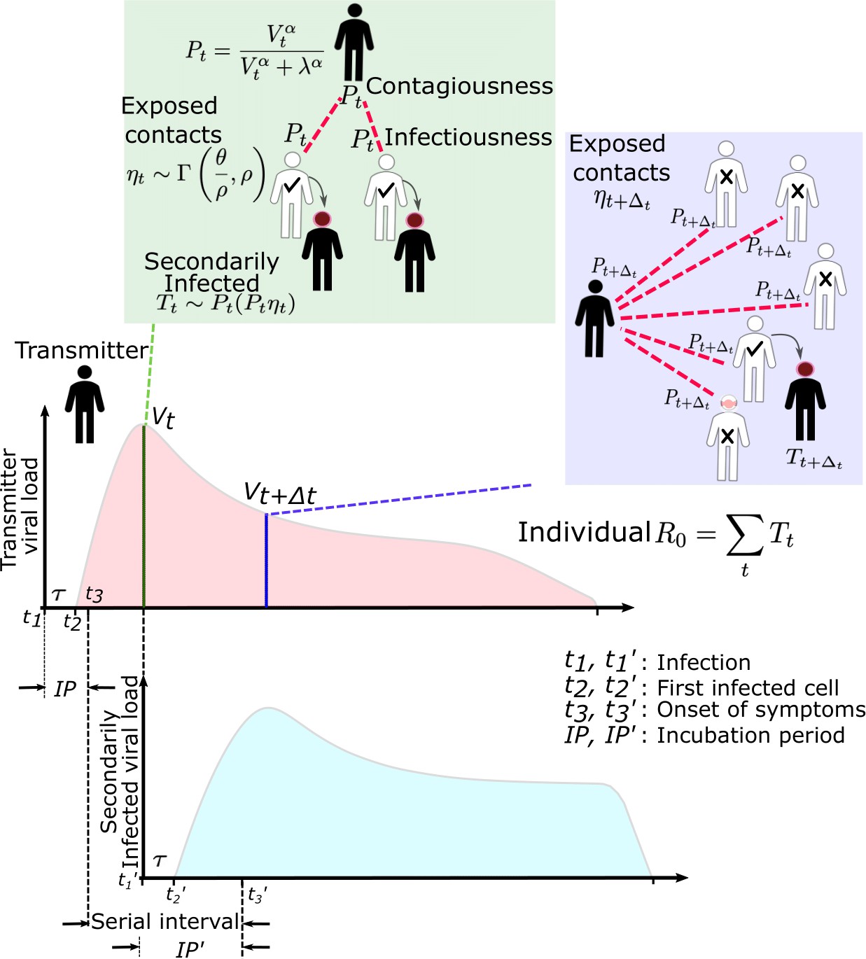
SARS-CoV-2 and influenza transmission model schematic.
In the above cartoon, the transmitter has two exposure events at discrete timepoints resulting in seven total exposure contacts and three secondary infections. Transmission is more likely at the first exposure event due to higher exposure viral load. To model this process, the timing of exposure events and number of exposed contacts is governed by a random draw from a gamma distribution which allows for heterogeneity in number of exposed contacts per day (Figure 1—figure supplement 3). Viral load is sampled at the precise time of each exposure event. Probability of transmission is identified based on the product of two dose curves (Figure 1—figure supplement 2c,d) which capture contagiousness (probability of viral passage to an exposure contact’s airway) and infectiousness (probability of transmission given viral presence in the airway). Incubation period (Figure 1—figure supplement 4) of the transmitter and secondarily infected person is an input into each simulation and is depicted graphically. Individual R0 is an output of each simulation and is defined as the number of secondary infections generated by an infected individual. Serial interval is an output of each simulated transmission and is depicted graphically.
Figure 1—figure supplement 1
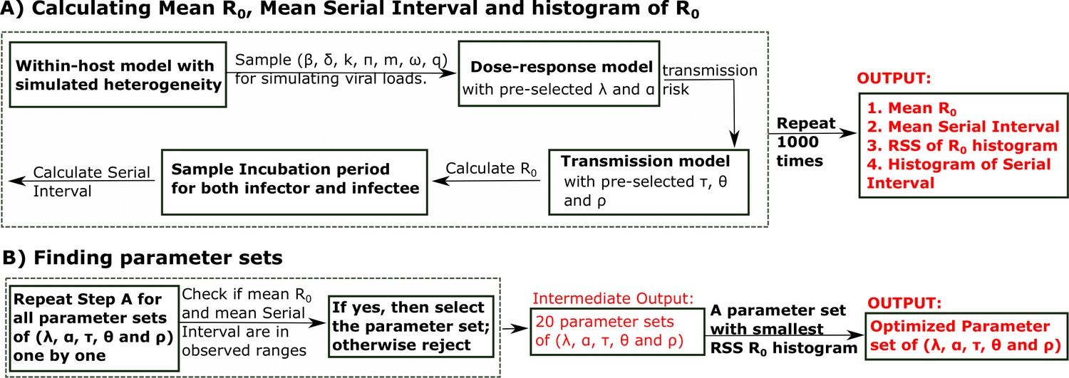
Mathematical model workflow.
Figure 1—figure supplement 2
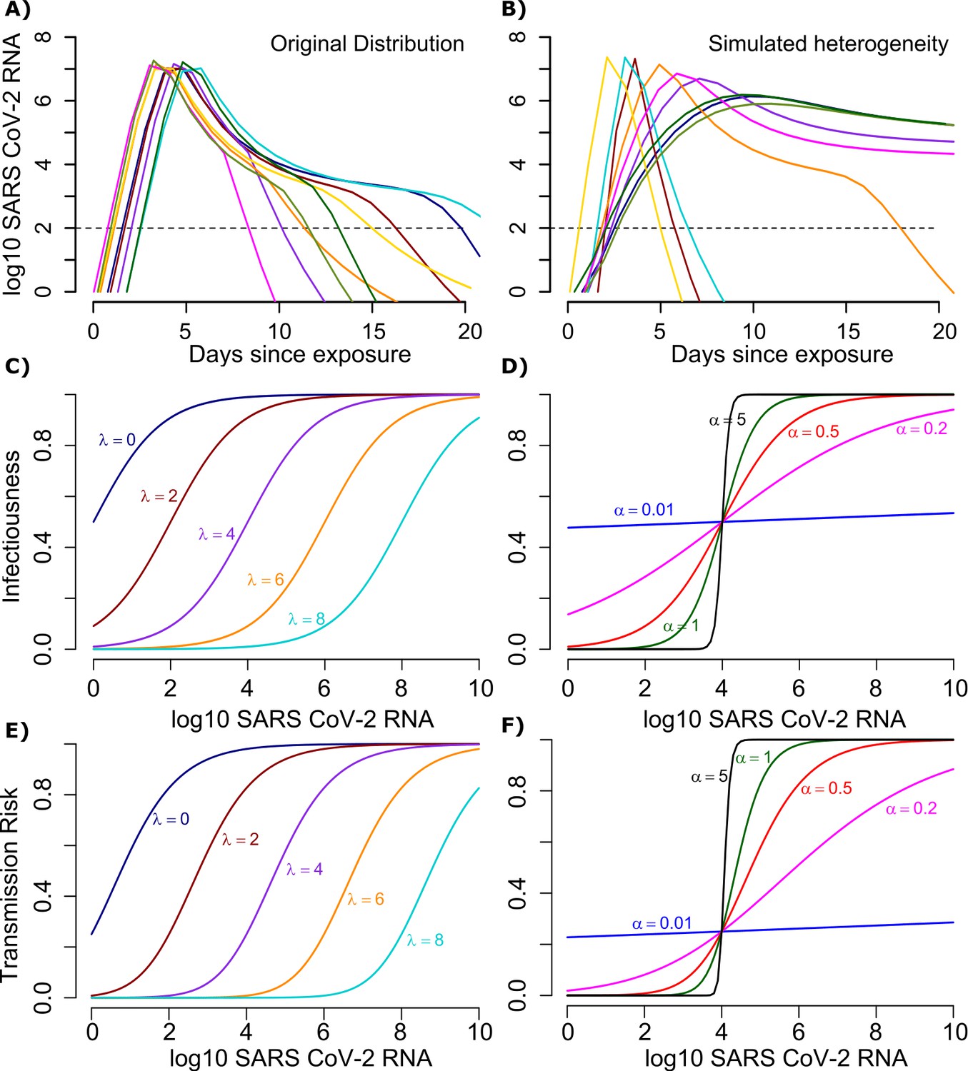
Mathematical model of SARS-CoV-2 transmission dynamics.
(A) Simulated viral load shedding tracings of possible transmitters. (B) Simulated viral load shedding with imputed heterogeneity. (C) Simulated infection dose (ID) response curves with variance in infectivity (ID50) and (D) dose response slopes. (E) Simulated transmission dose (TD) response curves with variance in infectivity (TD50) and (F) dose response slopes. The TD response curve is a product of the infection and contagion dose response curves. In (C) and (E), and in (D) and (F) .
Figure 1—figure supplement 3
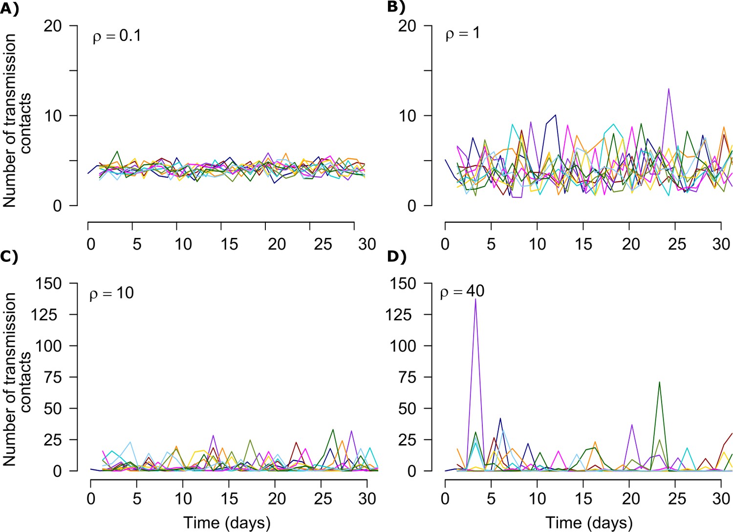
Stochastic simulations of the number of exposure contacts over time for varying dispersion (ρ).
The average number of exposed contacts is 4 per day in each example with imputed daily heterogeneity based on an elevated value of ρ. The number of exposure contacts at any time ‘t’ is drawn from a gamma distribution ~Γ(4/ρ, ρ). Different colored lines represent multiple instances of the number of exposure contacts over 30 days using the gamma distribution.
Figure 1—figure supplement 4
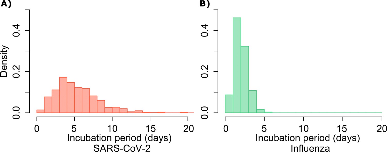
Gamma distribution functions of incubation periods.
(A) SARS-CoV-2 (mean 5.2 days, shape parameter = 3.45 and rate = 0.66) and (B) influenza (mean 2 days, shape parameter = 6.25 and scale parameter = 0.32).
Figure 2 with 1 supplement
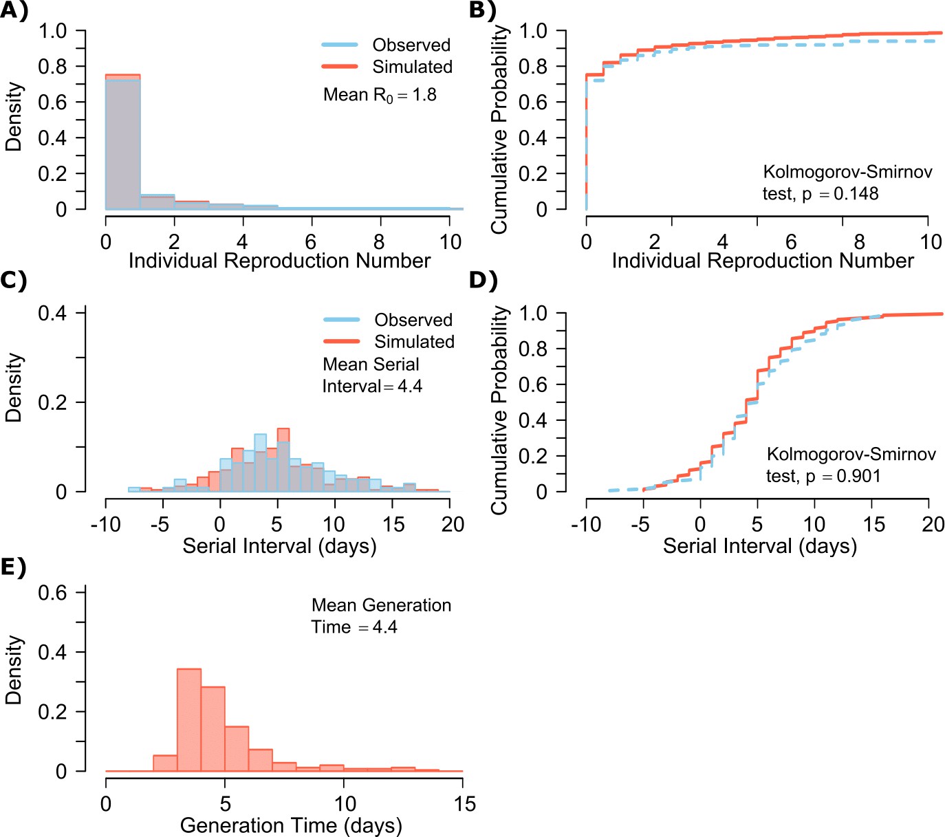
SARS-CoV-2 transmission model fit.
(A) Simulated and actual frequency histograms of individual R0 values, (Endo et al., 2020) (B) Simulated and actual cumulative distribution of individual R0 values. (C) Simulated and actual frequency histograms of individual serial intervals, (Du et al., 2020) (D) Simulated and actual cumulative distribution of individual serial intervals. (E) Frequency distribution of simulated generation times.
Figure 2—figure supplement 1
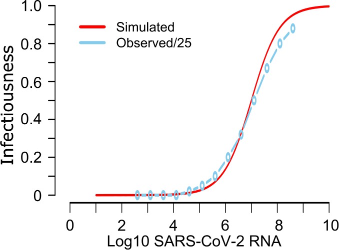
Mathematical model recapitulation of relationship between SARS-CoV-2 viral load and viral culture.
In a clinical study, probability of positive viral culture was projected against SARS-CoV-2 RNA (https://www.medrxiv.org/content/10.1101/2020.06.08.20125310v1). When we divided these PCR values by 25 (light blue line), we identified high similarity between the clinical data and our projected infectiousness dose response curve (red line).
Figure 3
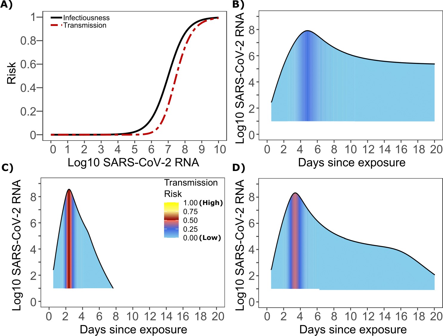
SARS-CoV-2 transmission probability as a function of shedding.
(A) Optimal infectious dose (ID) response curve (infection risk = Pt) and transmission dose (TD) response curve (transmission risk = Pt * Pt) curves for SARS-CoV-2. Transmission probability is a product of two probabilities, contagiousness and infectiousness (Figure 1). (B-D) Three simulated viral shedding curves. Heat maps represent risk of transmission at each shedding timepoint given an exposed contact with an uninfected person at that time.
Figure 4
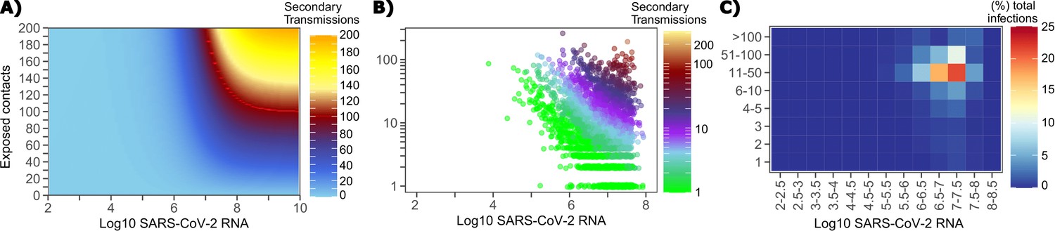
Conditional requirements for SARS-CoV-2 superspreading events.
(A) Heatmap demonstrating the maximum number of feasible secondary infections per day from a transmitter given an exposure viral load on log10 scale (x-axis) and number of exposed contacts per day (y-axis). The exposed contact network governed by the gamma distribution allows for a range of values between 0–200 per day with values > 200/day outside of the 99.99% quantile. Such high exposure contacts per day are sufficient for multiple transmissions from a single person per day. (B) 10,000 simulated transmitters followed for 30 days. The white space is a parameter space with no transmissions. Each dot represents the number of secondary transmissions from a transmitter per day. Input variables are log10 SARS-CoV-2 on the start of that day and number of contact exposures per day for the transmitter. There were 1,154,001 total simulated exposure contacts and 15,992 total infections. (C) 10,000 simulated transmitters with percent of infections due to exposure viral load binned in intervals of 0.5 intervals on log10 scale (x-axis) and number of exposed contacts (y-axis).
Figure 5
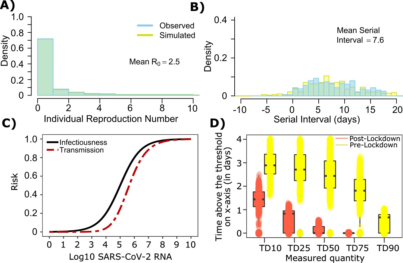
SARS-CoV-2 transmission model fit during the early phase of the pandemic in Wuhan.
(A) Simulated and observed frequency histograms of individual R0 values (Endo et al., 2020). (B) Simulated and actual frequency histograms of individual serial intervals (Li et al., 2020). (C) Optimal infectious dose (ID) response curve (infection risk = Pt) and transmission dose (TD) response curve (transmission risk = Pt * Pt) curves for SARS-CoV-2. (D) Boxplots of duration of time spent above TD10, TD25, TD50, TD75 and TD90 for 10,000 simulated SARS-CoV-2 infection during the early phase of pandemic (termed as pre-lockdown, before January 22, 2020) and post-lockdown (after January 22, 2020). TD10, TD25, TD50, TD75, and TD90 are viral loads at which transmission probability is 10%, 25%, 50%, 75%, and 90% respectively. The midlines are median values, boxes are interquartile ranges (IQR), and datapoints are outliers.
Figure 6

Influenza transmission model fit.
(A) Simulated and actual frequency histograms of individual R0 values (Brugger and Althaus, 2020). (B) Simulated and actual cumulative distribution of individual R0 values. (C) Simulated and actual frequency histograms of individual serial intervals (Cowling et al., 2009). (D) Simulated and actual cumulative distribution of individual serial intervals. (E) Frequency distribution of simulated generation times.
Figure 7
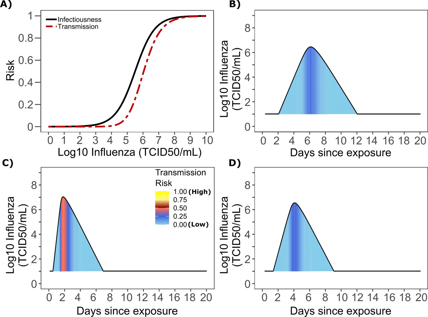
Influenza transmission probability as a function of shedding.
(A) Optimal infectious dose (ID) response curve (infection risk = Pt) and transmission dose (TD) response curve (transmission risk = Pt * Pt) curves for influenza. Transmission probability is a product of two probabilities, contagiousness and infectiousness (Figure 1). (B-D) Three simulated viral shedding curves. Heat maps represent risk of transmission at each shedding timepoint given an exposed contact with an uninfected person at that time.
Figure 8

Conditional requirements for influenza super spreading events.
(A) Heatmap demonstrating the maximum number of secondary infections per day feasible from a transmitter given an exposure viral load on log10 scale (x-axis) and number of exposed contacts per day (y-axis). (B) 10,000 simulated transmitters followed for 30 days. The white space is a parameter space with no transmissions. Each dot represents the number of secondary transmissions from a transmitter per day. Input variables are log10 influenza TCID on the start of that day and number of contact exposures per day for the transmitter. There are 1,239,984 total exposure contacts and 11,141 total infections. (C) 10,000 simulated infections with percent of infections due to exposure viral load binned in intervals of 0.5 intervals on log10 scale (x-axis) and number of exposed contacts (y-axis).
Figure 9 with 1 supplement
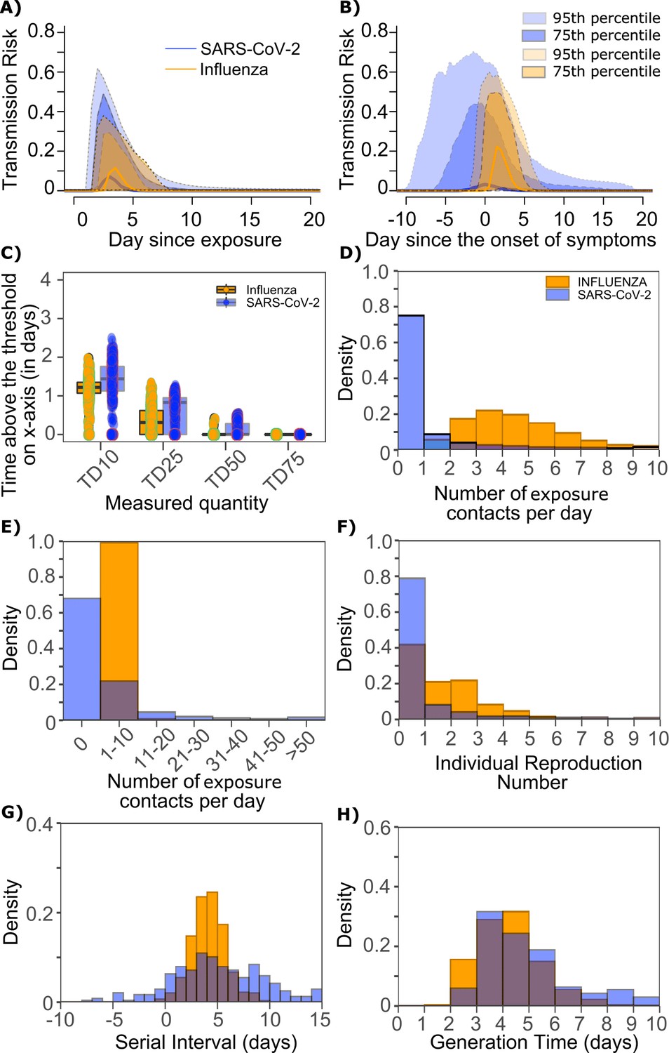
Differing transmission contact distributions, rather than viral kinetics explain SARS CoV-2 super spreader events.
(A) Simulated transmission risk dynamics for 10,000 infected persons with SARS-CoV-2 and influenza. Solid line is median transmission risk. Dark, dotted line is transmission risk of 75th percentile viral loads, and light dotted line is transmission risk of 95th percentile viral loads. (B) Same as A but plotted as transmission risk since onset of symptoms. Highest transmission risk for SARS-Co-V-2 is pre-symptoms and for influenza is post symptoms. (C) Boxplots of duration of time spent above TD10, TD25, TD50, TD75, and TD90 for 10,000 simulated SARS-CoV-2 and influenza shedding episodes. TD10, TD25, TD50, TD75, and TD90 are viral loads at which transmission probability is 10%, 25%, 50%, 75%, and 90%, respectively. The midlines are median values, boxes are interquartile ranges (IQR), and datapoints are outliers. Superimposed probability distributions of: (D and E) number of exposure contacts per day, (F) individual R0, (G) serial interval and (H) generation time for influenza and SARS-CoV-2.
Figure 9—figure supplement 1
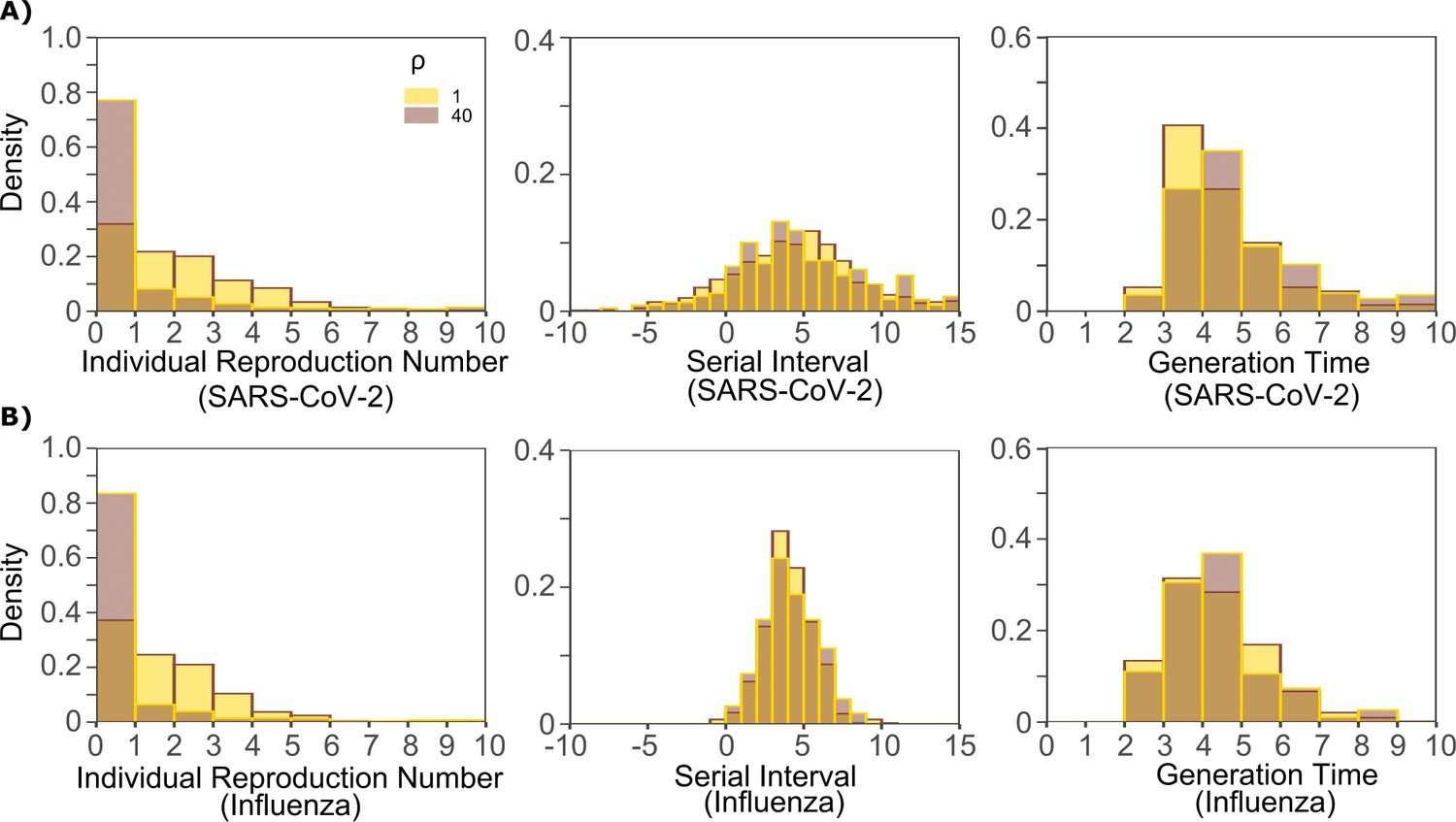
Impact of changes in contact network heterogeneity on individual R0, serial interval, and generation time.
(A) SARS-CoV-2 and (B) influenza. Lowering exposed contact network heterogeneity to levels observed with influenza decreases SARS-CoV-2 individual R0 over-dispersion. Increasing exposed contact network heterogeneity to levels observed with SARS-CoV-2 increases influenza R0 over-dispersion. Neither change impacts observed serial interval or estimate generation time.
Figure 10 with 5 supplements
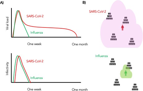
Wider dispersion of virus is the most likely explanation for SARS-CoV-2 super-spreader events.
(A) Despite differing shedding kinetics, our model projects very similar kinetics of infectivity between influenza and SARS-CoV-2 (Figure 9a,c) but (B) higher number of exposure contacts based on wider and / or more prolonged dispersal of virus creating potentialsws for super-spreader events.
Figure 10—figure supplement 1
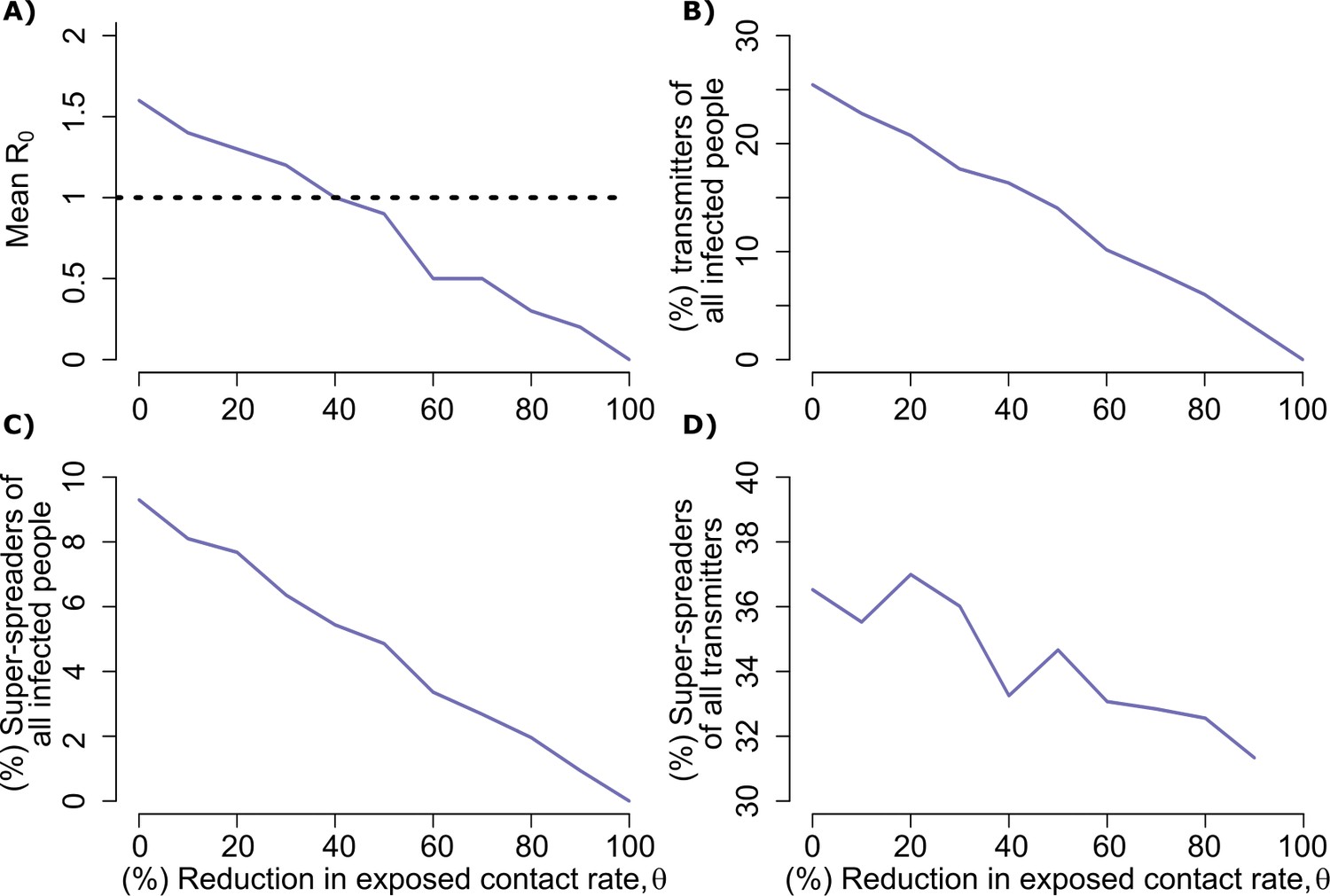
Potential impact of population physical distancing on SARS-Co-V2 epidemiology.
(A) Mean reproductive number (B) Percent transmitters of all infected people (C) Percent super-spreaders (individual R0 >5) of all infected people (D) Percent super spreaders of all transmitters. Transmitters are defined as infected people who generate at least one secondary infection.
Figure 10—figure supplement 2
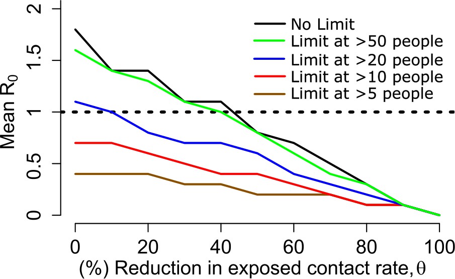
Potential impact of enhanced physical distancing only within high exposure contact networks on SARS-CoV-2 epidemiology.
Simulations assume limitation of exposed contacts only among daily exposures of more than 5, 10, 20, or 50 people. Mean reproductive number decreases below one with only marginal decreases in overall rate of exposure contacts when contacts are limited to fewer than 20 people.
Figure 10—figure supplement 3

Sensitivity analysis of transmission curve parameter for model fit to SARS-CoV-2 data.
Effects of varying transmission curve slope (x-axis) and TD50 for infectiousness (y-axis) on fit to (A) Mean R0, (B) Mean serial interval, (C) Cumulative distribution function of individual R0, and (D) Sum of Errors in A, B, and C.
Figure 10—figure supplement 4
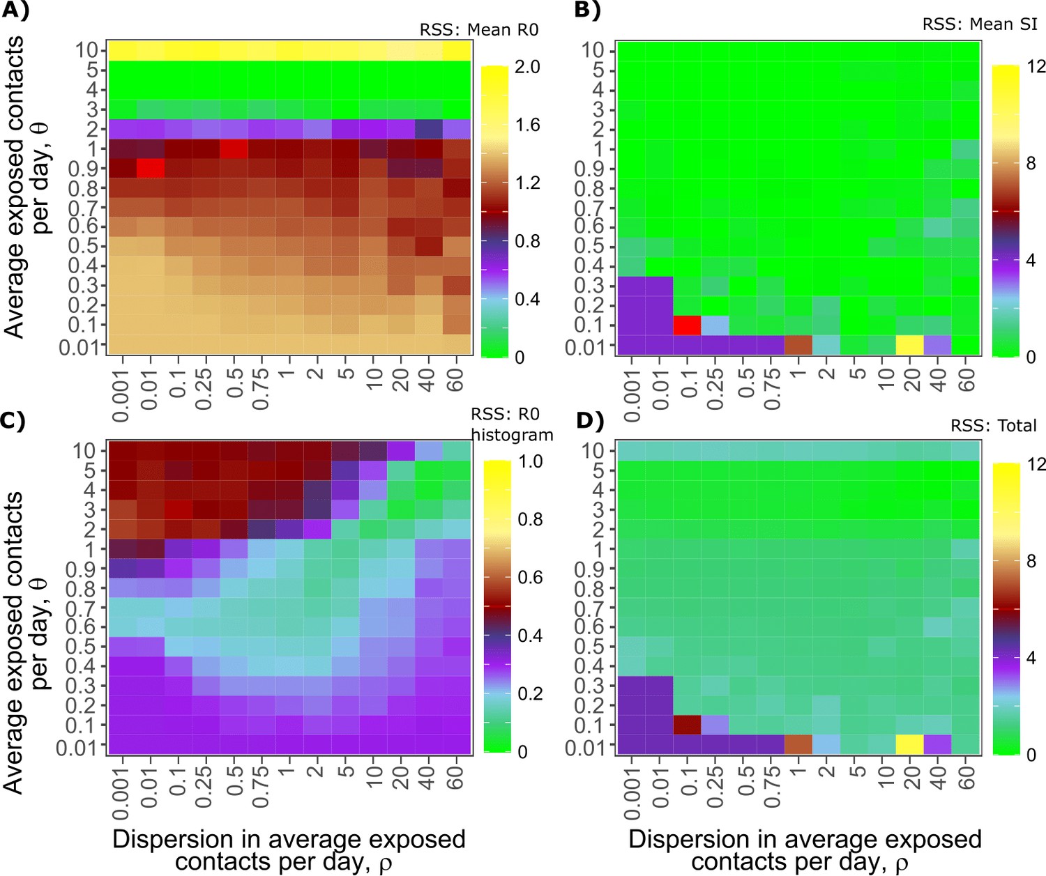
Sensitivity analysis of contact network structure for model fit to SARS-CoV-2 data.
Effects of dispersion parameter (x-axis) and average exposed contacts per day (y-axis) on fit to (A) Mean R0, (B) Mean serial interval, (C) Cumulative distribution function of individual R0, and (D) Sum of Errors in A, B, and C.
Figure 10—figure supplement 5

Histograms of four estimated parameters (, , , and ) using Approximate Bayesian Computation rejection sampling method.
In total, 1000 combinations of four parameters were obtained that fit the mean R0, mean SI and individual R0 histograms with a combined error of less than or equal to 0.1.
Author response image 1
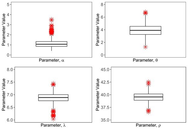
ABC approach to estimate 4 unknown parameters in the model.
We estimated 1000 parameter combinations of four parameters with an error threshold of 0.1 and showed them in the form of a boxplot.
Author response image 2
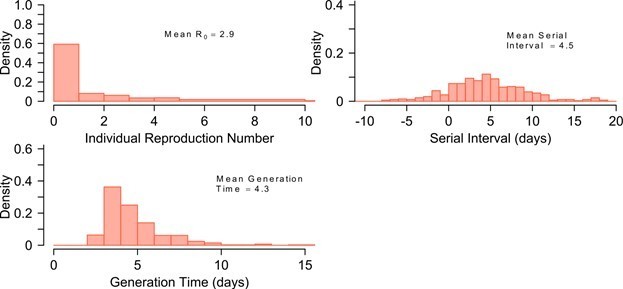
The distribution of individual R0, Serial Interval and Generation Time, when we assume data with higher R0 of 2.
8-2.9.
Tables
Table 1
Prevalence of super-spreaders among transmitters, and contribution of super-spreading events to all SARS-CoV-2 and influenza transmissions.
Estimates are from 10,000 simulations.
| Super-spreader definitions | SARS-CoV-2 | Influenza | ||||
|---|---|---|---|---|---|---|
| All infected people | All transmitters | Contribution of super-spreaders to transmissions | All infected people | All transmitters | Contribution of super-spreaders to transmissions | |
| Individual R0 ≥ 5 | ~10% | ~35% | ~85% | ~2% | ~3% | ~10% |
| Individual R0 ≥ 10 | ~6% | ~25% | ~70% | ~0% | ~0% | ~0% |
| Individual R0 ≥ 20 | ~2.5% | ~10% | ~44% | ~0% | ~0% | ~0% |
Table 2
Population parameter estimates for simulated SARS-CoV-2 viral shedding dynamics.
Parameters are from (doi: https://doi.org/10.1101/2020.04.10.20061325). The top row is the fixed effects (mean) and the bottom row is the standard deviation of the random effects. We also fixed r = 10, δE = 1/day, q = 2.4 × 10⁻⁵/day, and c = 15/day.
| Log10β (virions−1 day−1) | δ (day−1 cells-k) | k (-) | Log10π (log10 day−1) | m (day−1 cells−1) | Log10ω (day−1 cells−1) |
|---|---|---|---|---|---|
| −7.23 | 3.13 | 0.08 | 2.59 | 3.21 | −4.55 |
| 0.2 | 0.02 | 0.02 | 0.05 | 0.33 | 0.01 |
Additional files
Download links
A two-part list of links to download the article, or parts of the article, in various formats.
Downloads (link to download the article as PDF)
Open citations (links to open the citations from this article in various online reference manager services)
Cite this article (links to download the citations from this article in formats compatible with various reference manager tools)
Viral load and contact heterogeneity predict SARS-CoV-2 transmission and super-spreading events
eLife 10:e63537.
https://doi.org/10.7554/eLife.63537


