Figures and data in Multiple decisions about one object involve parallel sensory acquisition but time-multiplexed evidence incorporation

Figures
Tables
Additional files

8 figures, 7 tables and 1 additional file

Figures

Figure 1

Download asset Open asset

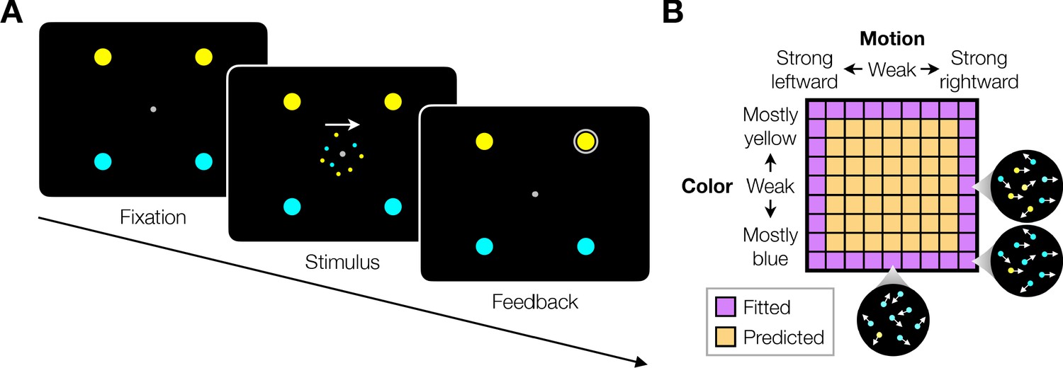
Double decision task.

(A) Timeline of the behavioral task. Participants fixated a gray dot at the center of the screen. A dynamic random dot stimulus was displayed and the participant was asked to judge the overall motion direction and the dominant color (the arrow is for visualization purposes only and was not presented to the subject). They reported this double-decision by selecting one of four targets to indicate motion direction (left and right target for leftward and rightward motion, respectively) and color (top yellow vs. bottom blue targets). The response was deemed correct when both motion and color judgments were correct. Participants received auditory feedback as to whether they were correct and the correct target was also indicated by a white ring. Across the experiments the targets could be selected with an eye movement or a hand movement, either when the participant was ready to report (reaction time) or when the dot display was extinguished (experimenter-controlled duration). (B) Motion and color strengths were varied independently across trials, represented by a matrix of combinations of difficulty levels (here shown for the eye reaction-time experiment with 81 combinations; see Materials and methods for Exp. 1-eye). Insets illustrate typical motion and color for three of the conditions. For feedback only, choices on the weakest motion strength (0% coherence) were deemed correct randomly; same for the weakest color strength. For the combinations shown in purple, at least one stimulus dimension was at its strongest value (easiest). For some analyses, the data from these combinations are used to fit a model, which is evaluated by predicting the data from the remaining combinations (amber).

Figure 2 with 6 supplements

Download asset Open asset

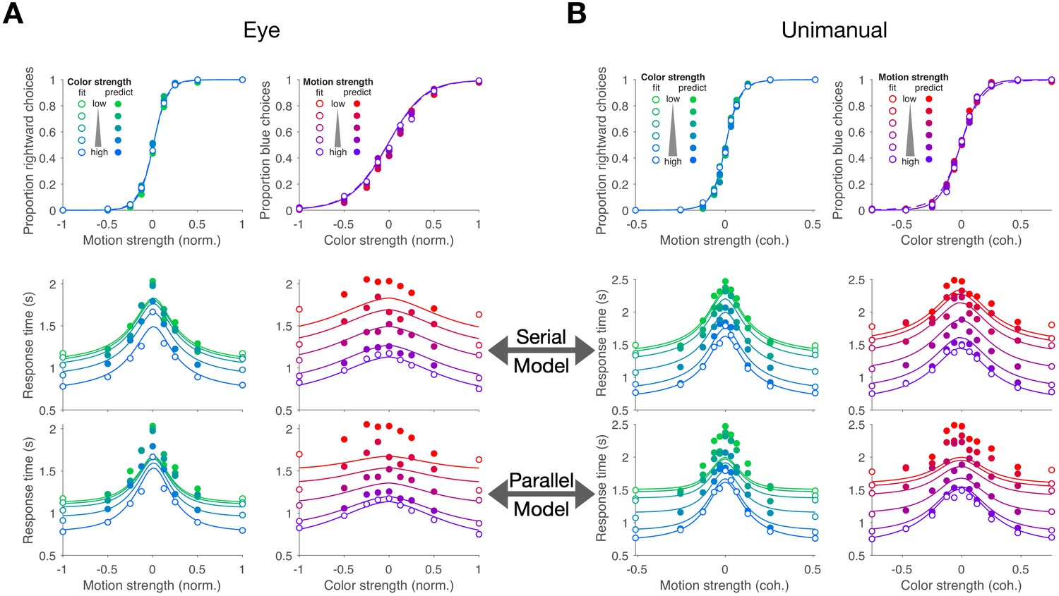
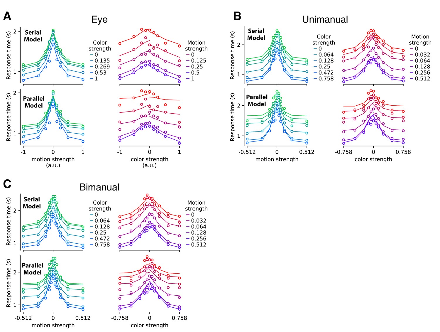
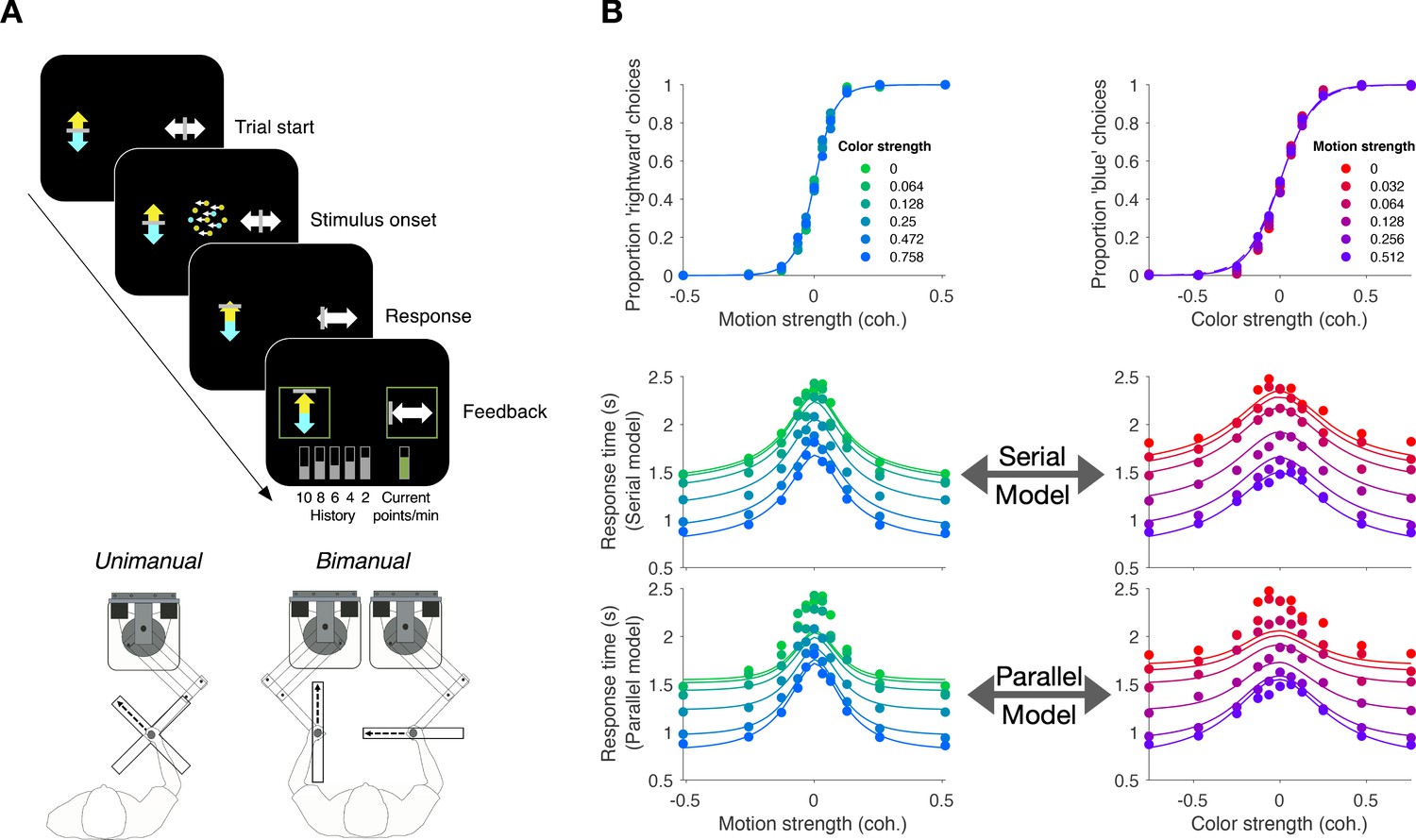
Double-decisions exhibit additive response times but no interference in accuracy (Experiment 1).

Participants judged the dominant color and direction of dynamic random dots and indicated the double-decision by an eye movement (A; Exp. 1-eye) or reach (B; Exp. 1-unimanual) to one of four choice-targets. All graphs show the behavioral measure (proportion of choices, top row; mean RT, rows 2 and 3) as a function of either signed motion or color strength. Positive and negative color strength indicate blue- or yellow-dominance, respectively. Positive and negative motion strength indicate rightward or leftward, respectively. Colors of symbols and traces indicate the difficulty (unsigned coherence) of the other stimulus dimension (e.g., color, for the graphs with abscissae labeled 'Motion strength'). Symbols are combined data from three participants (Exp. 1-eye) and eight participants (Exp. 1-unimanual). Open symbols identify the conditions used to fit the serial (middle row) and parallel (bottom row) models. These are the conditions in which at least one of the two stimulus strengths was at its maximum (purple shading, Figure 1B). In the top row, fits of the serial and parallel models are shown by solid and dashed lines, respectively. The models comprise two bounded drift-diffusion processes, which explain the choices and decision times as a function of either color or motion. They differ only in the way they combine the decision times to explain the double-decision RT. For the serial model, the double-decision time is the sum of the color and motion decision times. For the parallel model, the double-decision time is the longer of the color and motion decisions (see Materials and methods). Smooth curves are the predictions based on the fits to the open symbols. Both models predict no interaction on choice (top row). The predictions of RT are superior for the serial model (middle row) compared to the parallel model (bottom row). Data are the same in the lower two rows. Stimulus strengths in A were not identical for the three participants and were normalized to a common ±1 scale before averaging, so the psychometric curves for eye and hand cannot be compared visually (see Appendix 1—table 1 for comparison of parameters from the fits). For simplicity, only correct (and all 0% coherence trials) are shown in the RT graphs (see Materials and methods).

Figure 2—figure supplement 1

Download asset Open asset

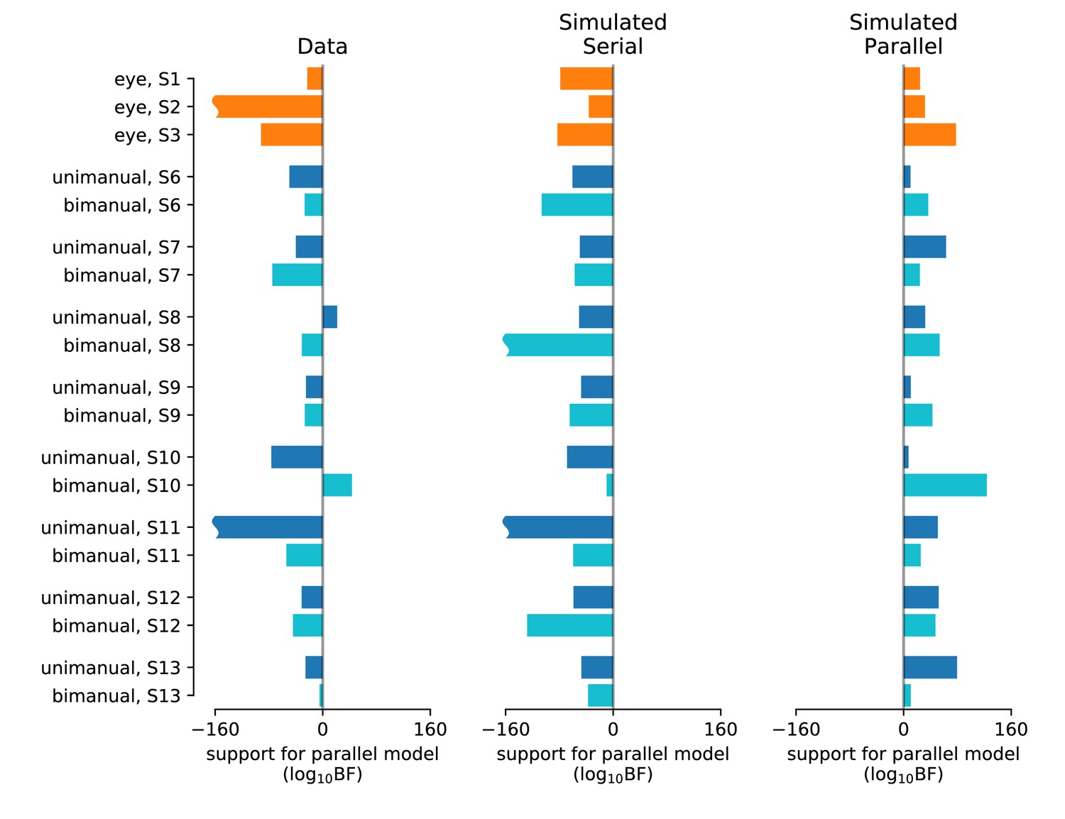
Statistical comparison of the drift diffusion model under serial vs. parallel rules (Experiments 1 and 4).

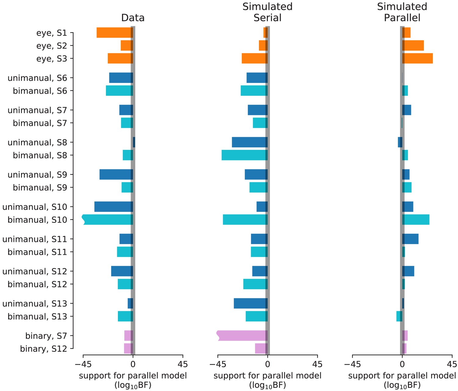
The analysis focuses on the data and predictions represented by the solid symbols and lines in Figure 2. *Left*, Difference in log likelihood of the predictions under parallel and serial rules for each participant and condition. Vertical gray shading centered at 0 encompasses ±2, corresponding to ‘decisive’ evidence (Bayes factor ≥ 100) in favor of serial (left extending bars) or parallel (right extending bars). *Middle and right*, Validation of the method. After fitting, these parameters were used to generate simulated data under the serial (left) and parallel (right) rules. Each dataset was then fit using both the serial and parallel rule. The validation shows that all simulated datasets were correctly categorized. Average $\log_{10} B F \pm S E M$ are −66 ± 26, –79 ± 14, and 42 ± 7 for the data, simulated serial, and simulated parallel, respectively. The magnitude of a wavy bars (e.g. eye, S2) exceeds the axis limit.

Figure 2—figure supplement 2

Download asset Open asset

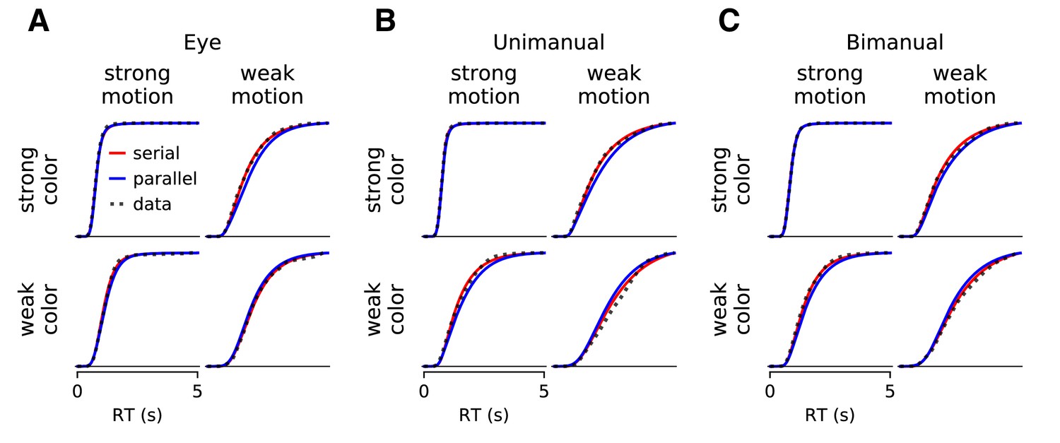
Comparison of parallel and serial rules applied to RT distributions (Experiments 1 and 4).

Instead of fits to drift-diffusion models, we employ an empirical approach to explain the observed distributions of double-decision RT by either additive or choose-max operations on unobserved distributions of color and motion decision times. The graphs show averages of the fitted cumulative distributions (thick colored traces) across participants. (A) Three participants who responded with an eye movement to one of four targets. (B) Eight participants who responded with a hand movement to one of four targets. (C) The same eight participants who responded with two hands (the RT is the time of the last movement). The averages are taken at each time bin across participants for each condition, weighted by the number of trials. Only the conditions with the weakest and strongest stimulus strengths are shown. The comparison provides decisive support for the serial combination rule (see Figure 2—figure supplement 3).

Figure 2—figure supplement 3

Download asset Open asset

Statistical comparison of parallel and serial rules applied to reaction time distributions (Experiments 1, 4, and 5).

The empirical analysis focuses on the full set of RT distributions, exemplified in Figure 2—figure supplement 2. The results are presented in the same format as Figure 2—figure supplement 1. Average $\log_{10} B F \pm S E M$ are −17 ± 3,–21 ± 2, 7 ± 2 for the data, simulated serial, and simulated parallel, respectively. For the binary-choice task (Experiment 5; pink), the simplified version of the RT model was used and 20 simulations were performed for each participant under the serial and parallel rule, respectively (bars represent the mean across the 20 simulations). For the remaining data, the full RT model was used and only a single serial/parallel simulation was performed for each participant. The magnitude of a wavy bars (e.g. bimanual, S10) exceeds the axis limit.

Figure 2—figure supplement 4

Download asset Open asset

Mean reaction time for parallel and serial rules applied to the empirical analysis of reaction time distributions exemplified in Figure 2—figure supplement 2 (Experiments 1 and 4).

The graphs display the mean RTs and fits in the same format as Figure 2, with responses reported by eye (A), unimanually (B), or bimanually (C). Mean RTs are computed from the average RT distribution computed as in Figure 2—figure supplement 2, and plotted with the same conventions as in Figure 2. Note that these averages across time bins and across participants are used for visualization only; fits were performed for individual participants using the full RT distribution. Here, the fits are derived from the best fitting gamma distributions, described in association with Figure 2—figure supplement 3. Open symbols are the data; the traces are line segments connecting the fitted means. In each panel of four graphs, the upper and lower pair of graphs show fits to the serial and parallel models, respectively. Panels display data from the double-decision RT tasks using the three response modalities as indicated.

Figure 2—figure supplement 5

Download asset Open asset

Application of the fit-prediction strategy in Figure 2 using only reaction time distributions.

The analysis is similar to the model comparison in Figure 2, where fits to the conditions in which at least one dimension was at its greatest strength (open symbols) are used to predict the mean double-decision RT on the remaining conditions (filled symbols), under serial and parallel rules. Instead of using a drift diffusion model to obtain the fitted 1D distributions, here we use the empirical method exemplified in Figure 2—figure supplement 2. Otherwise, same conventions as Figure 2—figure supplement 4.

Figure 2—figure supplement 6

Download asset Open asset

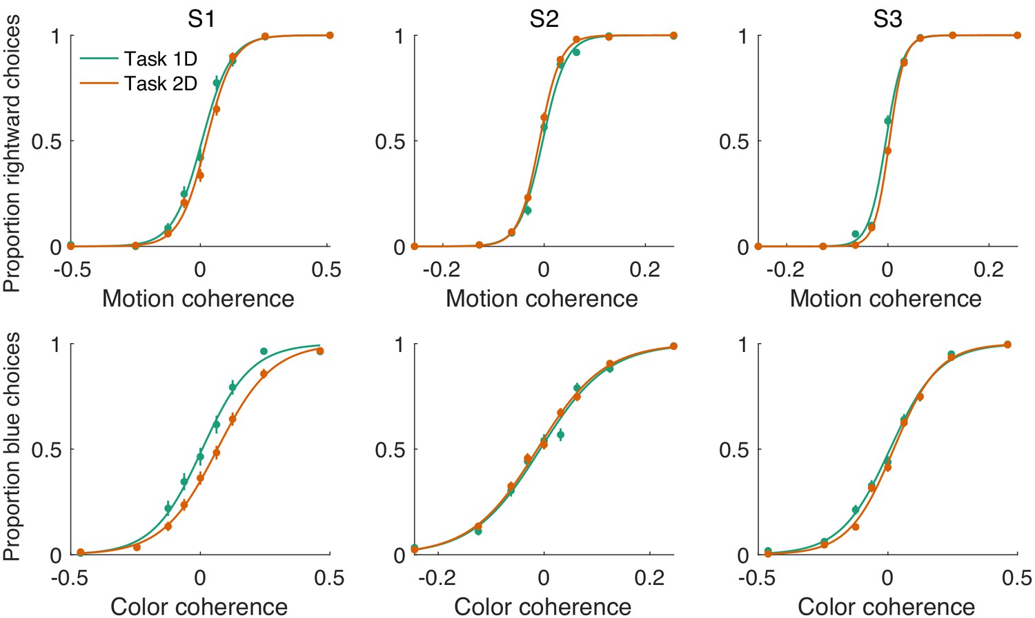
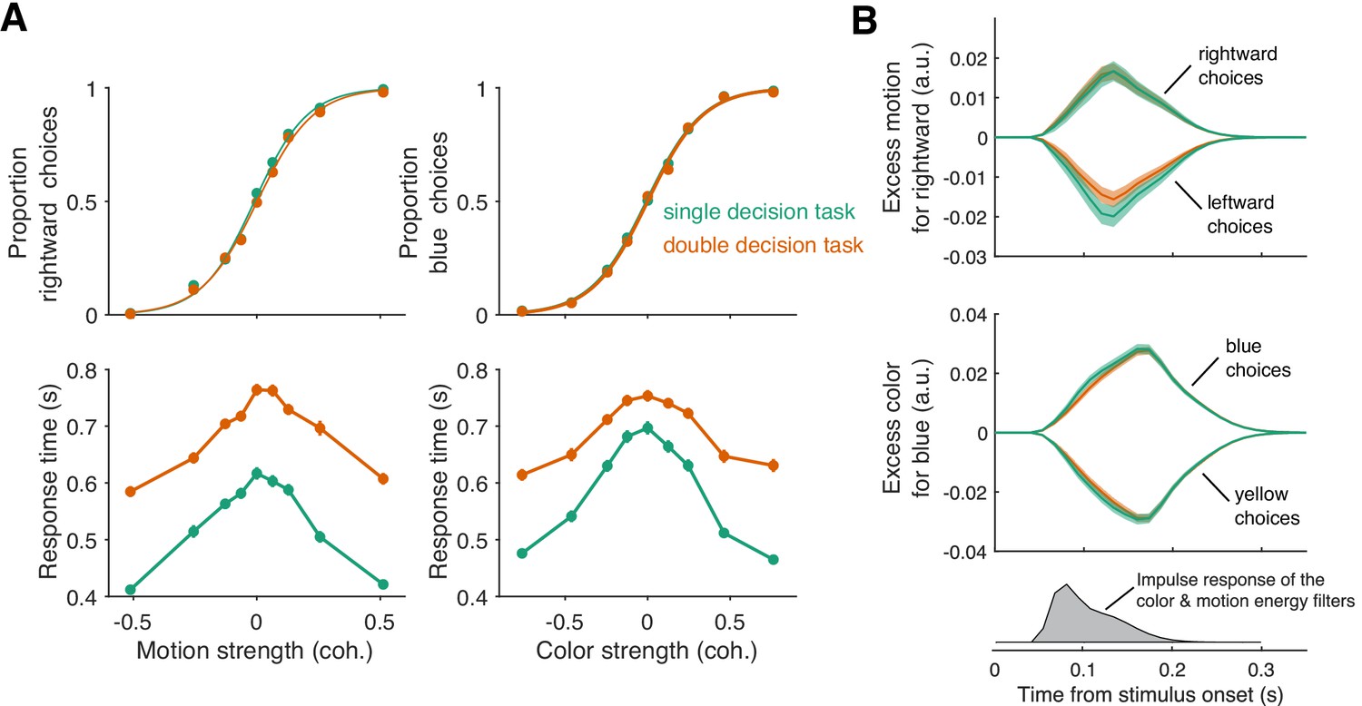
Sensitivity of color and motion choices on single-decision and double-decision tasks (Exp. 1-eye).

The proportion of rightward choices (*top row*) and blue choices (*bottom row*) are plotted as a function of stimulus strength. The data in green were obtained from blocks of trials in which the participant was instructed to answer only about one of the dimensions (motion or color) and to ignore the other dimension (color or motion). The displays and ranges of difficulty are the same as the ones used in the double-decision task. Data in orange were obtained from the double-decision task. The data are for eye-only as we did not include 1D blocks in the unimanual task. Sensitivity is the slope of a logistic fit to the data (see Appendix 1—table 4). The comparison is unprincipled because one does not expect the sensitivities to be the same for 1D decisions and the corresponding element of a 2D decision. The difference in task demands differ (e.g. error rates approach $\frac{1}{2}$ and $\frac{1}{4}$ for difficult 1D and 2D conditions), which could motivate different speed–accuracy settings. Nonetheless, they are comparable here.

Figure 3

Download asset Open asset

Parallel acquisition and serial incorporation of a brief color-motion pulse (Experiment 2).

Participants completed a short-duration variant of the double-decision task in which the stimulus was presented for only 120 ms. They also performed blocks in which they were asked to report only the color or only the motion direction (single decision in which they could ignore the irrelevant dimension). Data from double- and single-decision blocks are indicated by color. (A) Choices and RTs for single and double-decision blocks. *Top-left*, proportion of rightward choices as a function of motion strength. *Top-right*, proportion of blue choices as a function of color strength. The solid lines are logistic fits. They are nearly identical for single- and double-decisions. *Bottom row*, RT for the single- and double-decisions plotted as a function of motion strength (*left*) and color strength (*right*). For double-decisions, these are the same data plotted as a function of either the motion or color dimension. Data points show the average RT as a function of motion or color coherence, after grouping trials across participants and all strengths of the ‘other’ dimension (i.e. color, *left*; motion, *right*). Error bars indicate s.e.m. across trials. Although the stimulus was presented for only 120 ms, RTs were modulated by decision difficulty. Importantly, RTs were longer in the double-decision task than in the single-decision task. (B) Psychophysical reverse correlation analysis. *Top*, Time course of the motion information favoring rightward, extracted from the random-dot display on each trial, that gave rise to a left or right choice. Shading indicates s.e.m. *Middle*, Time course of the color information favoring blue, extracted from the random-dot display on each trial, that gave rise to a blue or yellow choice. Shading indicates s.e.m. The similarity of the green and orange curves indicates that participants were able to extract the same amount of information from the stimulus when making single- and double-decisions. *Bottom*, Impulse response of the filters used to extract the motion and color signals (see Materials and methods). They explain the long time course of the traces for the 120 ms duration pulse.

Figure 4 with 2 supplements

Download asset Open asset

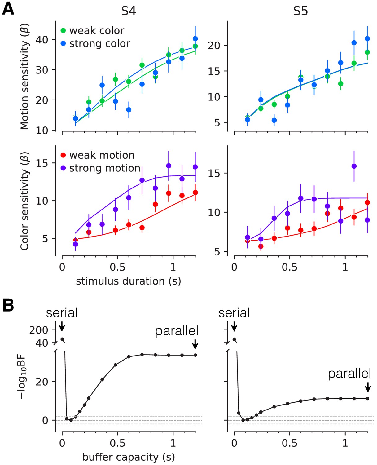
Interference in choice accuracy can be elicited at intermediate viewing durations (Experiment 3).

Two participants (columns) performed the color-motion double-decision task with a random dot display presented for 120–1200 ms. (A) *Top*, Motion sensitivity as a function of stimulus duration and color strength. Symbols are the slope of a logistic fit of the proportion of rightward choices as a function of signed motion strength, for each stimulus duration. Data are split by whether the color strength was strong (blue) or weak (green). Error bars are s.e. *Bottom*, Analogous color-sensitivity split by whether the motion strength was strong (purple) or weak (red). Curves are fits to the data from each participant using two bounded drift diffusion models that operate serially after an initial stage of parallel acquisition, here termed the buffer capacity. During the serial phase, one of the dimensions is prioritized until it terminates. The prioritization favored motion for both participants ( $p_{m}^{1 s t} = 0.80$ and 0.96, for participants S4 and S5, respectively). (B) Negative log likelihood of the model fits as a function of the buffer capacity, relative to the model fit at 80 ms capacity. The model is equivalent to a purely serial model, when the buffer capacity is zero, and to a purely parallel model when the buffer capacity exceeds the maximum stimulus duration. Negative log likelihoods were computed for a discrete set of buffer capacities (black points). Horizontal lines at $\log_{10} BF = 0$ indicate Bayes factor = 1. Dashed lines show where the Bayes factor = ± 100 (‘decisive’ evidence; Kass and Raftery, 1995).

Figure 4—figure supplement 1

Download asset Open asset

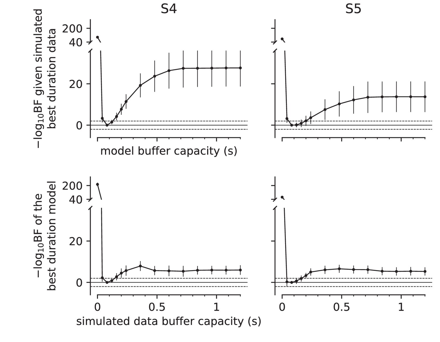
Parameter recovery analysis (Experiment 3).

The graphs evaluate the sensitivity and specificity of the estimates of buffer capacity ( $T_{buf}$ ) shown in Figure 4. Same plotting conventions as Figure 4B. Columns are the two participants. We used the parameters of the best fitting diffusion models to the data in Figure 4 (solid curves; see Appendix 1—table 5). The analysis in the top row addresses specificity. The simulations use 80 ms, but the model fits used $T_{buf}$ fixed to each of the durations shown on the abscissa, computed for a discrete set of buffer capacities (black points). The ordinate shows the difference of each model's negative log likelihood from that of the 80 ms buffer model (smaller is better). Error bars are standard deviations across 12 simulations. The analysis suggests fiducial confidence limits of roughly 80–200 ms. The analysis in the bottom row addresses identifiability. The simulations use $T_{buf}$ shown on the abscissa. We then compare two fits, using $T_{buf} = 80$ ms or the simulated value. Misidentification is limited to a narrow range similar to the fiducial confidence interval.

Figure 4—figure supplement 2

Download asset Open asset

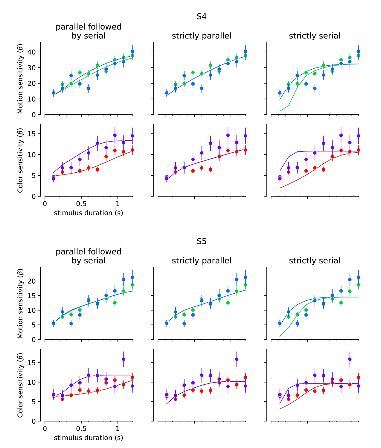
Fits to the choice data in Experiment 3 with strictly serial and parallel models.

The best fitting model to the choice data in the variable duration task implicates a finite buffer, allowing motion or color information to be held for a period before updating the decision. If $T_{buf} = \infty$ or 0, the model is purely parallel or purely serial. The graphs show the best fits of these models for two subjects. The format of the graphs is identical to Figure 4. *Left column*, reproduction of the fits in Figure 4. *Middle column*, best fitting parallel model. *Right column*, best fitting serial model.

Figure 5 with 2 supplements

Download asset Open asset

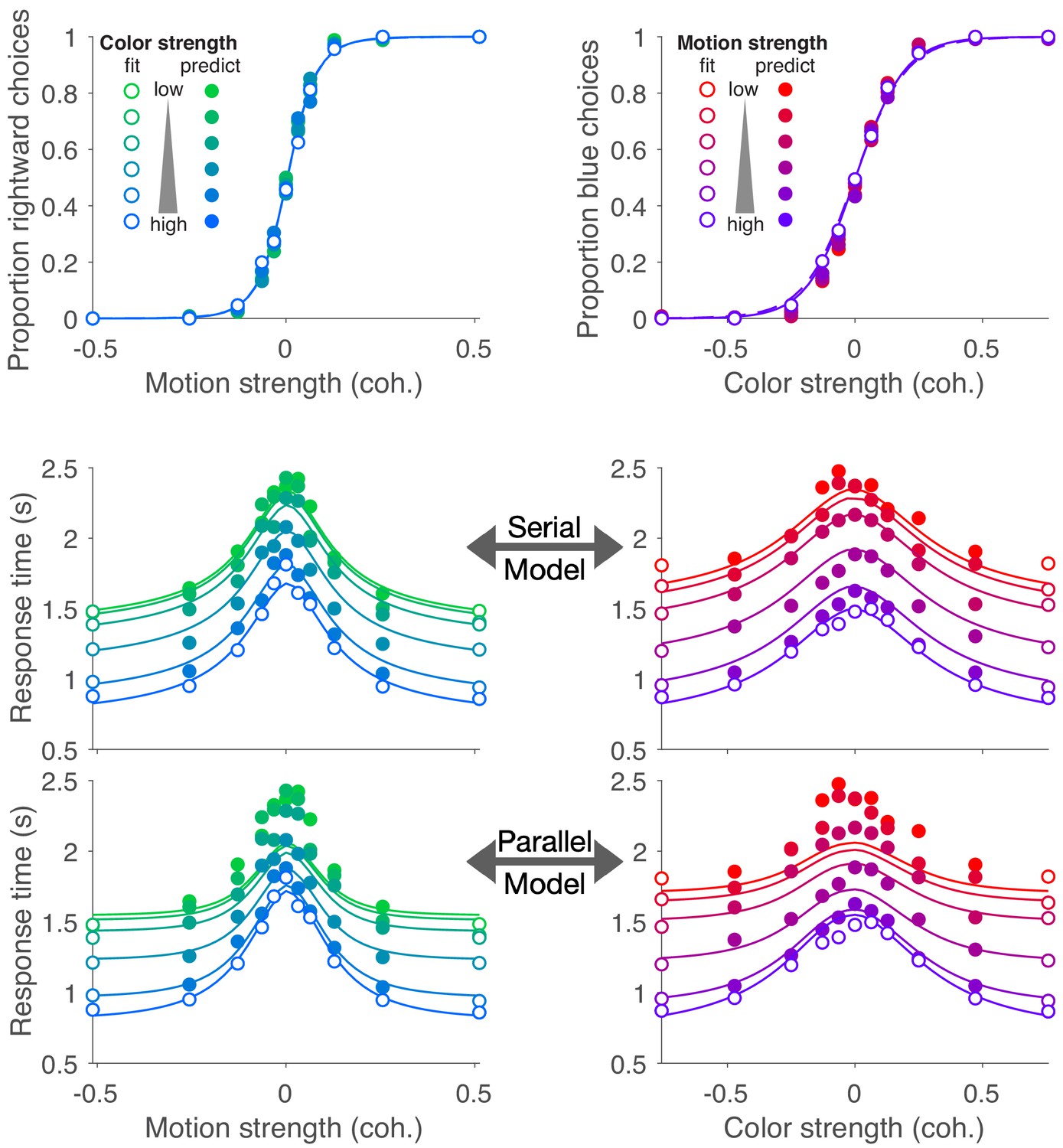
Replication of double-decision choice-reaction time when the decisions are reported with two effectors (Experiment 4).

(A) Participants performed the color-motion double-decision choice-reaction task, but indicated the double-decision with either a unimanual movement to one of four choice-targets or a bimanual movement in which each hand reports one of the stimulus dimensions (N = 8 participants performed both tasks in a counterbalanced order). In both conditions, the hand or hands were constrained by a robotic interface to move only in directions relevant for choice (rectangular channels). The display was the same in the unimanual and bimanual tasks, with up-down movement reflecting color choice and left-right movement reflecting motion choice. A scrolling display of proportion correct was used to encourage accuracy. In the unimanual trials both choices were indicated simultaneously. However, in the bimanual trials each choice could be indicated separately and the dot display disappeared only when the second hand left the home position. (B) Choice proportions and double-decision mean RT on the bimanual task. The double-decision RT on the bimanual task is the latter of the two hand movements. The data are plotted as a function of either signed motion or color strength (abscissae), with the other dimension shown by color (same conventions as in Figure 2). Solid traces are identical to the ones shown in Figure 2B for the unimanual task, generated by the method of fitting the conditions containing at least one stimulus condition at its maximum strength and predicting the rest of the data. They establish predictions for the bimanual data from the same participants. The agreement supports the conclusion that the participants used the same strategy to solve the bimanual and unimanual versions of the task. Note that a few symbols are occluded by others.

Figure 5—figure supplement 1

Download asset Open asset

Choice and double-decision RT for the bimanual responses (Experiment 4) in the same format as Figure 2B.

These are the same data shown in Figure 5 but replacing the predictions from the unimanual fits with the fits to the data from the bimanual task. We use the same fit/prediction strategy as in Figure 2B. The model comparison is summarized in Figure 2—figure supplement 1.

Figure 5—figure supplement 2

Download asset Open asset

Model-free comparison of performance in the unimanual (blue) vs. bimanual (red) task (Experiment 4).

(A) *Top:* Sensitivity of color choices as a function of motion strength (unsigned coherence). Sensitivity is the slope of a logistic regression of color choice as a function of signed color coherence, obtained separately for each level of motion strength. *Bottom:* RTs in the uni- vs. bimanual task as a function of motion strength when color was weak (three lowest strengths; light shading) vs. strong (three highest strengths; dark shading). For the bimanual task, RTs correspond to the final response of a given trial. (B) Similar to A, but with the roles of color and motion swapped in the analysis. *Top:* motion sensitivity. *Bottom:* RTs as a function of color strength when motion was either weak (light shading) or strong (dark shading). No differences in overall choice sensitivity were found between the uni- and bimanual task (repeated-measures ANOVA, motion sensitivity: F_1,7 = 0.21, p=0.664; color sensitivity: F_1,7 = 0.70, p=0.431). Similarly, overall RTs were similar in the uni- and bimanual task (motion: F_1,7 = 0.56, p=0.477; color: F_1,7 = 0.57, p=0.476). Furthermore, the modulation of RTs by the informative and uninformative dimensions, respectively, was not affected by task (uni-/bimanual; all interactions p > 0.05). This suggests that overall performance, and modulation of RTs by each decision dimension, were similar in the uni- and bimanual tasks. Data points represent mean ± s.e.m. (N = 8).

Figure 6

Download asset Open asset

First response times in the bimanual task suggest multiple switches in decision updating (Experiment 4).

For bimanual double-decisions, participants indicate two RTs per trial. Whereas up to now we have only considered the RT corresponding to completion of both color and motion decisions, the analyses in this figure concern the RT of the first of the two. Symbols are means ± s.e. (N = 8 participants). Curves are fits to single- and multi-switch model (orange and blue, respectively). (A) RT as a function of motion strength when motion was reported first. (B) RT as a function of color strength when motion was reported first. (C) RT as a function of motion strength when color was reported first. (D) RT as a function of color strength when color was reported first. In panels A and D, the first response corresponds to the stimulus dimension represented on the abscissa. The data exhibit the expected pattern of fast RT when the stimulus is strong and slow RT when the stimulus is weak (i.e. near 0). This would occur if the serial processing of motion and color ensued one after the other (single-switch) or with more than one alternation (multi-switch), although the latter provides a better account of the data. In panels B and C, the first response corresponds to the stimulus dimension that is not represented on the abscissa. Here the single-switch model fails to account for the data. If there were only one switch and color terminates first, then the strength of motion is irrelevant, because all processing time was devoted to color. Similarly, if there were only one switch and motion terminates first, then the strength of color is irrelevant, because all processing time was devoted to motion.

Figure 7 with 1 supplement

Download asset Open asset

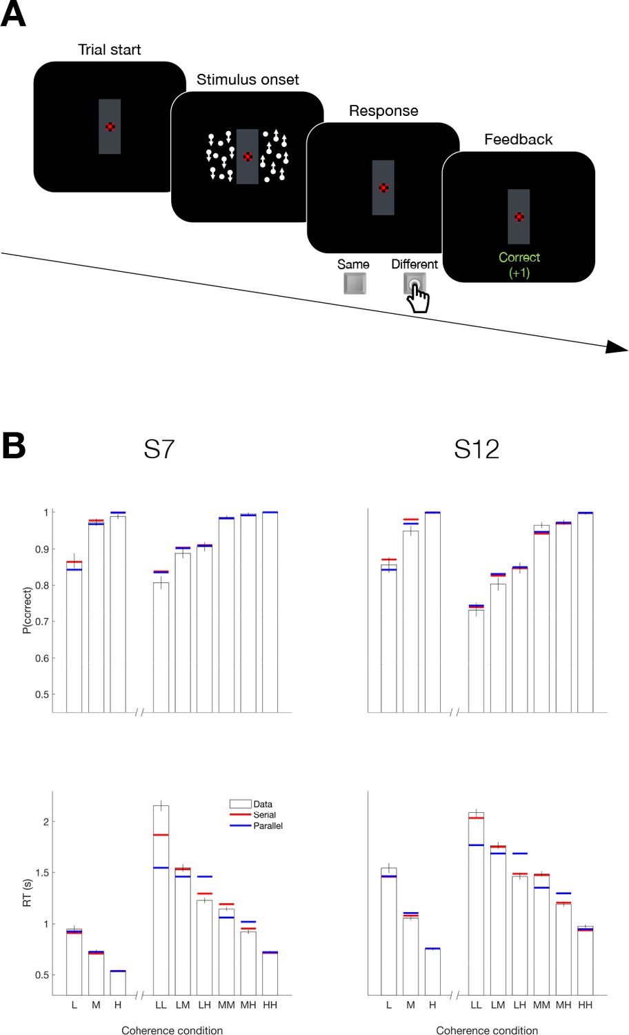
Serial decision making in a Same vs. Different task (Experiment 5).

(A) Task. Two dynamic random dot motion displays were presented in rectangular patches to the left and right of a central fixation cross. The direction and motion strength were randomized from trial to trial and between the patches (up or down × three motion strengths). Participants judged whether the dominant direction of the left and right patches is the same or different and indicated the decision when ready by pressing a response key with their left or right index finger. At the end of each trial, participants received feedback. In a separate block, participants also performed a 1D direction discrimination task in which only one patch of random dots was displayed. (B) Results and fits for two participants (columns). *Top*, Proportion of correct choices as a function of the level of motion strength (i.e. unsigned coherence; L = low; M = medium; H = High). *Bottom*, Response times for each level of motion strength. The first three bars represent the direction task where only a single motion stimulus was presented. The six bars on the right of each plot represent the same-different task. Horizontal red and blue lines are fits of serial and parallel drift-diffusion models to the means. Only correct trials were included for RT analyses.

Figure 7—figure supplement 1

Download asset Open asset

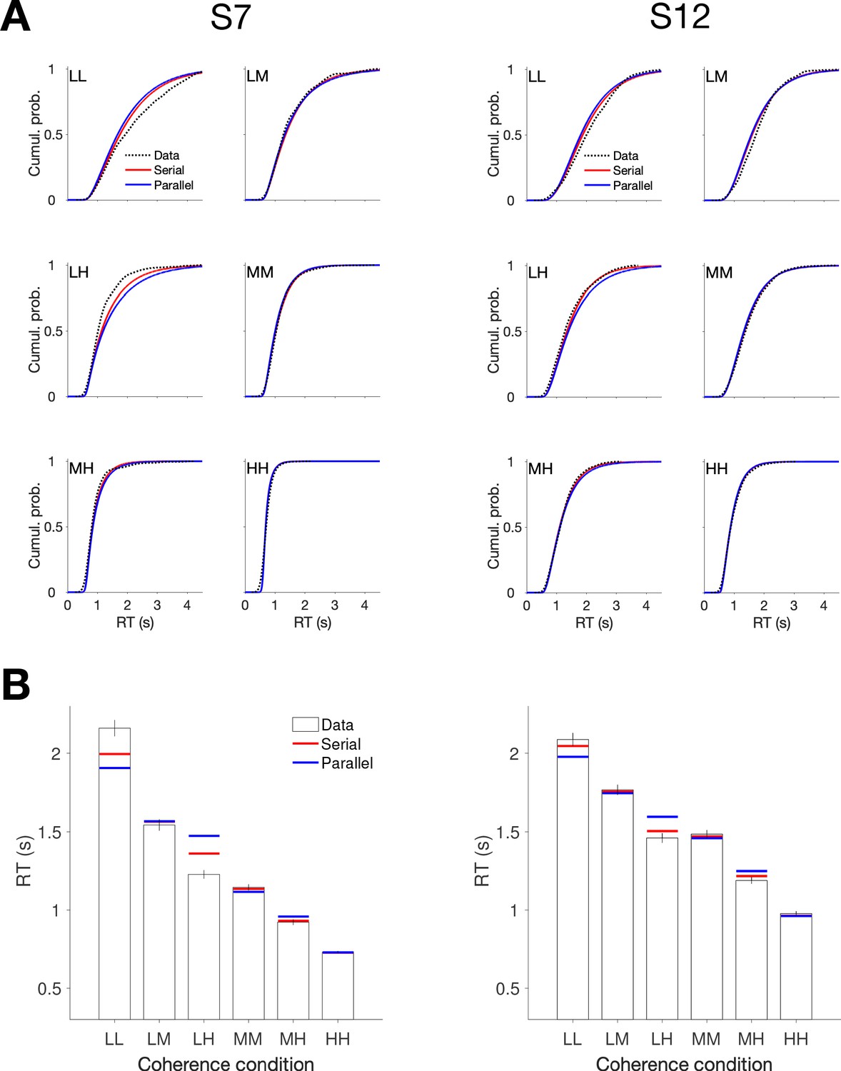
Comparison of parallel and serial rules applied to reaction time distributions in the Same vs Different task (Experiment 5).

Comparison of parallel and serial rules applied to reaction time distributions in the Same vs. Different task (Experiment 5). The analysis is a variant of the empirical approach introduced in Figure 2—figure supplement 2, applied to RT distributions associated with the six unique combinations of motion strength (correct choices only). The analysis optimizes the parameters of gamma distributions representing three 1D decision times, corresponding to the three unique motion strengths, and one non-decision time to best explain the six observed distributions of RTs. (A) Best fitting RT distributions for each participant, shown as cumulative probability distributions. Dashed black curves are data. Solid curves are best fitting distributions under serial (red) and parallel (blue) combination rules. (B) Superposition of the expectations obtained from the fitted distributions (panel A) on the mean RT.

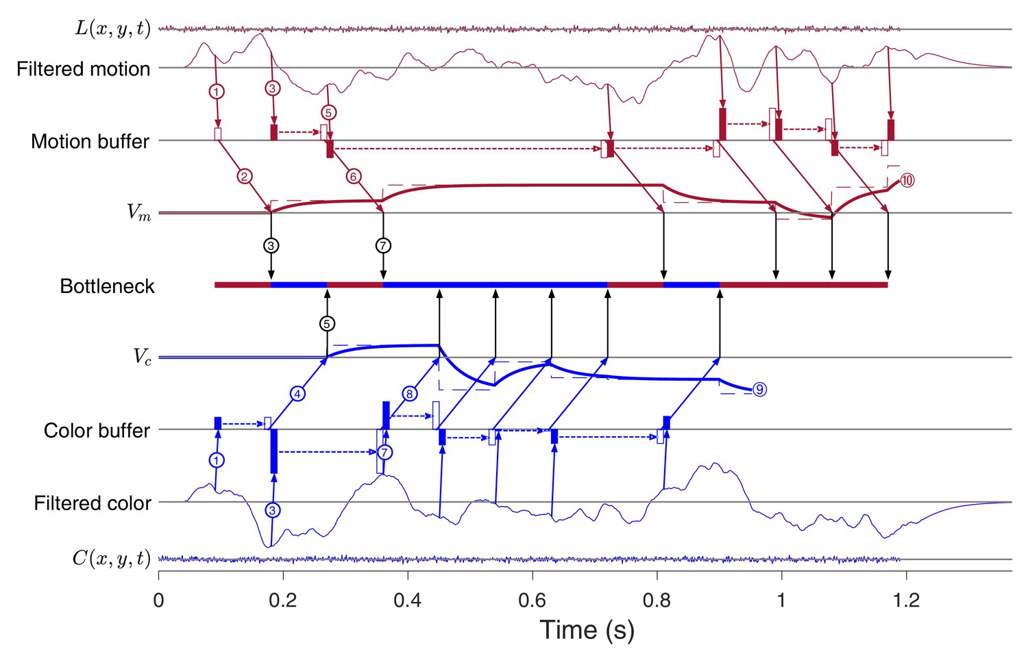
Figure 8 with 3 supplements

Download asset Open asset

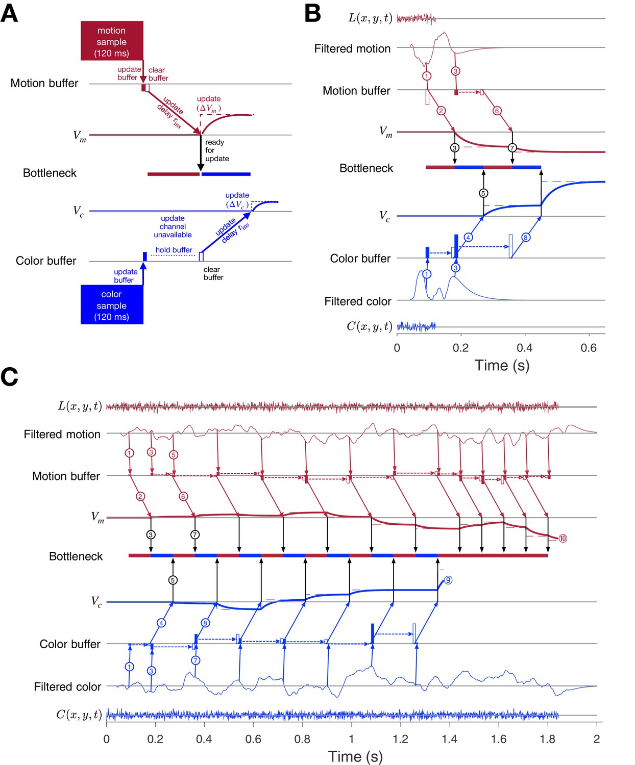
Parallel acquisition of evidence and serial updating of two decision variables.

An elaborated drift diffusion model permits reconciliation of the serial processing implied by the double-decision choice-RT experiment and the failure to observe interference in choice accuracy when the color-motion stimulus is restricted to a brief pulse. The main components of the model are introduced in panel A and elaborated in panels B and C. In all panels, maroon and blue indicate motion and color processes, respectively. (A) Simulated trial from the short duration experiment (Experiment 2). Information flows from top to middle graphs for motion; and from bottom to middle graphs for color. Time is left to right. The evidence from both color and motion is extracted from the 120 ms random dot stimulus in parallel. Both can be stored temporarily in separate buffers (filled rectangles), which send an instruction to the circuits representing the respective decision variables in their persistent firing rates. The instruction is to change the firing rate by an amount ( $Δ V_{m}$ or $Δ V_{c}$ ). This latency from clearance of the sample from the buffer to receipt of the $Δ V$ instruction takes time ( $τ_{ins}$ , diagonal arrows), and this is followed by the realization of the instruction in the evolving firing rates of cortical neurons (smooth colored curves). In the example, the $V_{m}$ is the first to update. A central bottleneck precludes updating $V_{c}$ . The bottleneck is unblocked when the $Δ V_{m}$ instruction is received by the circuit that represents the motion decision variable (black arrow). This allows the buffered evidence for color to update $V_{c}$ . Open rectangle represents clearance of the buffer content, which occurs immediately for motion and after a delay for color in this example. Dashed lines associated with the decision stage show the instructed change in the decision variable ( $Δ V_{m}$ and $Δ V_{c}$ ). Smooth colored curves show the evolution of the decision variables. (B) Elaboration of the example in panel-A. The boxes representing the 120 ms stimulus are replaced by the two outer rows: (i) raw luminance and color data stream, $L (x, y, t)$ and $C (x, y, t)$ , respectively, represented as biased Wiener processes (duration 120 ms); (ii) filtered evidence streams containing the relevant motion (right minus left) and color (blue minus yellow) signals. The filters introduce a delay and smoothing. The filtered signals can be sampled by the buffer every $τ_{s}$ ms, so long as the buffer is available (i.e. empty). The bottleneck shows the process that is accessing the update channel. Other than the first sample, the prioritization is equal and alternating. Only one process can update at a time. Circled numbers identify the key events described in Results. Events sharing the same number are approximately coincidental. (C) Example of a double-decision in the choice-RT task. The first eight steps parallel the logic of the process shown in panel B. The decision variables then continue to update serially, in alternation, until $V_{c}$ reaches a terminating bound ⑨. The decisions then continues as a single-dimension motion process until $V_{m}$ reaches a terminating bound (⑩). Note that the sampling rate is the same as it was in the parallel phase, whereas during alternation it was half this rate for each dimension. Bound height is indicated by ⑨ and ⑩.

Figure 8—figure supplement 1

Download asset Open asset

Example of a 1D choice-reaction time trial.

The model in Figure 8 retains compatibility with 1D decisions. The example uses identical settings to those in Figure 8, but there is only a color decision. Samples are acquired every $τ_{s} = 90$ ms, and the buffer is cleared immediately. Notice that the decision variable, $V_{c}$ , does not reflect evidence until $τ_{s} + τ_{ins} = 180$ ms, which is similar to the latency observed in LIP and prefrontal cortex (Huk and Shadlen, 2005; Kim and Shadlen, 1999). The bottleneck is blocked while the content of the buffer is transmitted to $V_{c}$ (i.e. for $τ_{ins}$ ; angled arrows from buffer to $V_{c}$ ), and this implies that for all samples after the first, $τ_{s}$ should equal $τ_{ins}$ , else some evidence could be missed. For example, suppose that a second sample were obtained at $t = 0.12$ s. It would be held until the bottleneck was unblocked, at $t = 0.18$ s, and this would miss 60 ms of evidence. From here on, the buffer can only be filled once it is cleared and this imposes the equality of $τ_{s}$ and $τ_{ins}$ , as in the late phase of motion processing in Figure 8C.

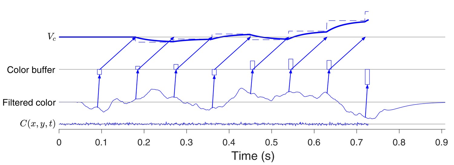
Figure 8—figure supplement 2

Download asset Open asset

Example of a 2D decision with one switch after parallel acquisition.

After the parallel acquisition phase, motion is prioritized until termination at ⑧, which removes the bottleneck, allowing for the the next update of $V_{c}$ , sampled at ③ ( $t = 0.18$ s) and buffered until ⑧. The 1D color decision-process continues until termination at ⑩. The example approximates the drift-diffusion model used to fit data from Experiment 3. (Same conventions as in Figure 8C).

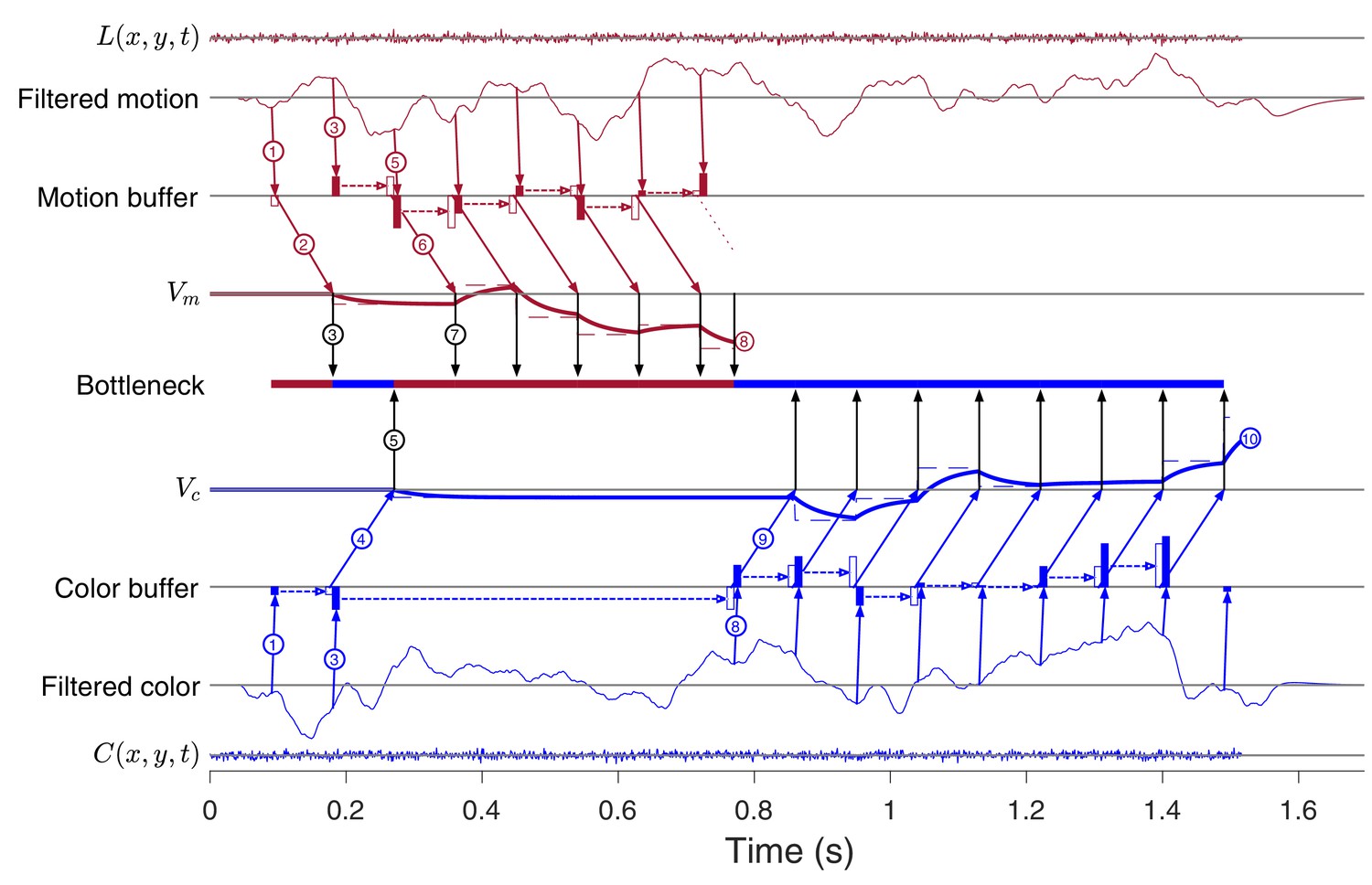
Figure 8—figure supplement 3

Download asset Open asset

Example of a 2D decision with stochastic switching.

After the parallel acquisition phase (as in Figure 8B,C) there are three color samples obtained in succession, followed by a alternation to motion then color then motion. While this last motion was transmitted to instruct $Δ V_{m}$ , the color decision terminated at ⑨, thereby allowing for the final phase of motion sampling with termination at ⑩. Note that the final buffer clearance would only instruct $Δ V_{m}$ after decision termination. It could affect post-decision processes, such as change of mind (Resulaj et al., 2009) or confidence. (Same conventions as in Figure 8C).

Tables

Table 1

Experimental parameters.

Experiment 1. Double-decision reaction time (eye and unimanual), Experiment 2. Brief stimulus presentation (eye), Experiment 3. Variable-duration stimulus presentation (eye), Experiment 4. Two-effector double-decision reaction time (bimanual) and Experiment 5. Binary-response double-decision reaction time.

	Exp 1.-eye	Exp 2.	Exp 3.	Exp 1.-uni. & Exp 4.	Exp 5.
Dot density (dots deg^-2 s^-1)	15.3	15.3	16	16	16
Dot speed (deg/s)	1.67	1.67	5	5	5
Dot diameter (deg)	0.075	0.075	0.061	0.082	S7: 0.098; S12: 0.119
Fixation marker diameter (deg)	0.4 gray circle	0.4 gray circle	0.6 red cross and bullseye	0.6 red cross and bullseye	0.6 red cross and bullseye
Random delay (s)	0.1–0.5	0.1–0.5	0.5–0.8	0.5–0.8	0.4–0.8
Visual target diameter (deg)	0.4	0.4	1.2	N/A	N/A
Target eccentricity (deg)	6	6	15	N/A	N/A
Movement initiation	gaze > 2.5°	gaze > 2.5°	gaze > 3°	hand > 1 cm	key press
Target detection window (radius)	3°	3°	2.4°	0.75 cm	N/A
CRT	Vision Master 1451	Vision Master 1451	Sony CRT CPD-G420S	Dell CRT P1110	N/A
Refresh rate (Hz)	75	75	75	75	60
Resolution (pixels)	1400 × 1050	1400 × 1050	1280 × 1024	1280 × 1024	S7: 1280 × 720; S12: 1440 × 900
Pixels per degree	39.6	39.6	32.7	24.3	S7: 40.94; S12: 33.45
Viewing distance (cm)	55	55	50	38	S7: 54; S12: 38
Blue $c d / m^{2}$ [M(SD)]	N/A	N/A	25.20 (0.81)	12.16 (1.93)	N/A
Blue CIE x/y [M]	N/A	N/A	x = 0.26, y = 0.24	x = 0.27, y = 0.24	N/A
Yellow $c d / m^{2}$ [M(SD)]	N/A	N/A	22.98 (0.05)	12.68 (1.80)	N/A
Yellow CIE x/y [M]	N/A	N/A	x = 0.54, y = 0.38	x = 0.54, y = 0.38	N/A

Table 2

Motion and color strength parameters.

For 2D trials all combinations of motion and color strengths were used. For 1D trials all strengths were used for the dimension that informed the decision but some strengths ( $^{*}$ ) were omitted for the other dimension.

Experiment	Participant	Motion strengths	Color strengths
1. Double-decision RT (eye)	S1	0, 0.064, 0.128, 0.256, 0.512	0, 0.062, 0.124, 0.245, 0.462
	S2	0, 0.032, 0.064, 0.128, 0.256	0, 0.031, 0.062, 0.124, 0.245
	S3	0, 0.032, 0.064, 0.128, 0.256	0, 0.062, 0.124, 0.245, 0.462
2. Brief stimulus presentation (eye)	S1–3	0, 0.064, 0.128, 0.256, 0.512	0, 0.124, 0.245, 0.462, 0.762
3. Variable-duration stimulus presentation (eye)	S4	0.03, 0.063, 0.512	0.052, 0.104, 0.758
3. Variable-duration stimulus presentation (eye)	S5	0.044, 0.084, 0.512	0.046, 0.104, 0.758
4. Two-effector double-decision reaction time (bimanual, same strengths for unimanual)	S6–13	0, 0.032, 0.064, 0.128, 0.256, 0.512	0, 0.064, 0.128, 0.250, 0.472, 0.758
5. Binary-response double-decision RT	S7 and S12	0.128, 0.256, 0.512	N/A

Appendix 1—table 1

Parameter values for the best-fitting serial model (Experiments 1 and 4).

Note that the rate of collapse parameters ( $a_{m}$ and $a_{c}$ ) are limited to a maximum of 10 (an almost instantaneous bound collapse) and the time of the start of the collapse ( $d_{m}$ and $d_{c}$ ) are limited to 4 s.

Task	Subj.	$κ_{m}$	$u_{m}$	$a_{m}$	$d_{m} (s)$	$s_{m}^{0}$	$κ_{c}$	$u_{c}$	$a_{c}$	$d_{c} (s)$	$s_{c}^{0}$	$μ_{n d} (s)$	$σ_{n d} (s)$
Eye RT	1	9.97	0.98	6.45	3.47	−0.02	5.77	0.83	10	4	−0.01	0.3	0.001
	2	21.99	0.99	3.65	2.52	0.01	11.39	0.68	10	2.61	0.02	0.35	0.002
	3	39.25	0.83	9.91	3.26	−0.01	6.29	3.62	1.23	−0.19	0	0.31	0.004
Unimanual	6	14.02	1.3	1.97	3.96	0.01	7.24	0.91	3.09	2.18	0.04	0.34	0.001
	7	13.94	1.42	2.01	3.6	−0.01	4.97	1.33	1.21	2.79	0.06	0.41	0.001
	8	9.98	1.11	4.07	4	0	7.16	1.03	2.15	2.93	0.02	0.31	0.001
	9	12.84	0.75	10	2.64	0	7.18	0.91	10	3.28	0.02	0.69	0.08
	10	20.81	0.88	10	4	−0.01	7.46	0.91	3.72	2.14	−0.06	0.37	0.001
	11	19.56	0.84	4.81	2.72	0	7.67	1.73	0.32	0.51	−0.03	0.42	0.004
	12	12.05	0.96	2.51	3.98	0	5.28	0.96	10	3.35	0.03	0.44	0.001
	13	13.13	1	2.67	4	−0.02	5.87	1.06	0.98	3.06	0.02	0.41	0.001
Bimanual	6	8.39	0.74	10	3.44	0	4.36	0.98	10	4	0.04	0.33	0.001
	7	9.45	0.8	10	4	−0.02	4.56	0.97	7.67	3.92	0.05	0.3	0.001
	8	11.89	1.44	0.65	1.64	−0.04	6.9	1.03	1.78	1.85	−0.02	0.37	0.007
	9	13.57	0.87	10	4	0	7.05	0.86	4.57	2.49	−0.1	0.44	0.002
	10	13.03	1.34	1.51	3.84	0	6.9	1.07	2.1	2.81	0.07	0.38	0.022
	11	12.56	1.68	0.77	2.35	0	6.78	0.95	2.32	3.05	0.05	0.46	0.001
	12	12.65	1.03	6.16	3.33	0.01	6.01	1.08	10	3.96	−0.03	0.31	0.001
	13	8.91	1.16	5.14	3.91	0.01	4.25	1.05	1.42	3.87	−0.09	0.3	0.001

Appendix 1—table 2

Parameter values for the best-fitting switching model (Experiment 4–bimanual).

Subj.	$τ_{Δ} (s)$	$p_{m}^{1 s t}$	$T_{n d}^{1 s t} (s)$
6	1.48	0.5	0.42
7	0.88	0.33	0.59
8	8.73	0.86	0.38
9	1.27	0.88	0.43
10	0.16	0.05	0.38
11	0.18	0.86	0.71
12	0.22	0.6	0.5
13	0.74	0.92	0.64

Appendix 1—table 3

Parameter values for the best-fitting drift-diffusion model (Experiment 5–binary-choice).

Task	Subj.	$κ_{m}$	$B_{0}^{1 D}$	$B_{0}^{2 D}$	$s_{m}^{0}$	$T_{n d}^{1 D} (s)$	$T_{n d}^{2 D} (s)$
Binary choice	7	8.96	0.85	1.09	0.03	0.35	0.24
Binary choice	12	6.83	1.17	1.03	−0.04	0.43	0.35

Appendix 1—table 4

Sensitivity of color and motion choices obtained on single decision and double-decision tasks.

Eye-RT. Sensitivity is the slope of a logistic fit to the proportion of rightward (blue) choices as a function of motion (color) strength. Values in the 1D columns are obtained from different blocks in which participants were instructed to answer only the motion direction or color dominance. Values in the 2D columns are obtained from the double-decisions, using either the motion or color choice. Binary choice. Here, the 2D task refers to the same-different task. Sensitivity for the 1D task is the slope of a logistic fit to direction choices for one patch (ignoring the other). For the same-different task, the direction choices on individual patches is not reported. The 1D sensitivity is estimated by fitting the proportion of same and different choices assuming the same sensitivity to motion direction for each patch. Parentheses show s.e.

		Motion sensitivity		Color sensitivity
Task	Subj.	1D task	2D task	1D task	2D task
Eye-RT	S1	17.5 (3.0)	18.7 (0.8)	10.6 (0.7)	9.5 (0.5)
	S2	43.4 (10.9)	48.1 (2.1)	15.8 (0.7)	16 (0.5)
	S3	59 (2.0)	68.2 (1.8)	10.5 (0.4)	11.5 (0.3)
Binary choice	S7	13.3 (1.0)	13.9 (1.0)
Binary choice	S12	13.2 (0.9)	19.3 (1.6)

Appendix 1—table 5

Parameter values for the best-fitting buffer + serial model (Experiment 3–Variable-duration stimulus presentation).

Task	Subj.	$κ_{m}$	$u_{m}$	$g_{m} (s)$	$d_{m} (s)$	$s_{m}^{0}$	$κ_{c}$	$u_{c}$	$g_{c} (s)$	$d_{c} (s)$	$s_{c}^{0}$	$p_{m}^{1 s t}$	$T_{b u f} (s)$
VD	4	22.29	0.86	0.47	1.19	0.01	9.18	1.39	0.18	0.27	−0.01	0.80	0.08
VD	5	9.60	0.99	0.68	0.40	0.01	12.11	0.74	0.11	0.11	0.04	0.96	0.08

Additional files

Transparent reporting form: https://cdn.elifesciences.org/articles/63721/elife-63721-transrepform-v2.docx
Download elife-63721-transrepform-v2.docx

Download links

A two-part list of links to download the article, or parts of the article, in various formats.

Downloads (link to download the article as PDF)

Open citations (links to open the citations from this article in various online reference manager services)

Mendeley

Cite this article (links to download the citations from this article in formats compatible with various reference manager tools)

Yul HR Kang
Anne Löffler
Danique Jeurissen
Ariel Zylberberg
Daniel M Wolpert
Michael N Shadlen

(2021)

Multiple decisions about one object involve parallel sensory acquisition but time-multiplexed evidence incorporation

eLife 10:e63721.

https://doi.org/10.7554/eLife.63721

Share this article

Cite this article

Double decision task.

Double-decisions exhibit additive response times but no interference in accuracy (Experiment 1).

Statistical comparison of the drift diffusion model under serial vs. parallel rules (Experiments 1 and 4).

Comparison of parallel and serial rules applied to RT distributions (Experiments 1 and 4).

Statistical comparison of parallel and serial rules applied to reaction time distributions (Experiments 1, 4, and 5).

Mean reaction time for parallel and serial rules applied to the empirical analysis of reaction time distributions exemplified in Figure 2—figure supplement 2 (Experiments 1 and 4).

Application of the fit-prediction strategy in Figure 2 using only reaction time distributions.

Sensitivity of color and motion choices on single-decision and double-decision tasks (Exp. 1-eye).

Parallel acquisition and serial incorporation of a brief color-motion pulse (Experiment 2).

Interference in choice accuracy can be elicited at intermediate viewing durations (Experiment 3).

Parameter recovery analysis (Experiment 3).

Fits to the choice data in Experiment 3 with strictly serial and parallel models.

Replication of double-decision choice-reaction time when the decisions are reported with two effectors (Experiment 4).

Choice and double-decision RT for the bimanual responses (Experiment 4) in the same format as Figure 2B.

Model-free comparison of performance in the unimanual (blue) vs. bimanual (red) task (Experiment 4).

First response times in the bimanual task suggest multiple switches in decision updating (Experiment 4).

Serial decision making in a Same vs. Different task (Experiment 5).

Comparison of parallel and serial rules applied to reaction time distributions in the Same vs Different task (Experiment 5).

Parallel acquisition of evidence and serial updating of two decision variables.

Example of a 1D choice-reaction time trial.

Example of a 2D decision with one switch after parallel acquisition.

Example of a 2D decision with stochastic switching.

Experimental parameters.

Motion and color strength parameters.

Parameter values for the best-fitting serial model (Experiments 1 and 4).

Parameter values for the best-fitting switching model (Experiment 4–bimanual).

Parameter values for the best-fitting drift-diffusion model (Experiment 5–binary-choice).

Sensitivity of color and motion choices obtained on single decision and double-decision tasks.

Parameter values for the best-fitting buffer + serial model (Experiment 3–Variable-duration stimulus presentation).

Transparent reporting form

Downloads (link to download the article as PDF)

Open citations (links to open the citations from this article in various online reference manager services)

Cite this article (links to download the citations from this article in formats compatible with various reference manager tools)